The virtual-spot approach: a simple method for image U–Pb carbonate geochronology by high-repetition-rate LA-ICP-MS

We present a simple approach to laser ablation inductively coupled plasma mass spectrometry (LA-ICP-MS) U–Pb dating of carbonate minerals from isotopic maps, made possible using a high-repetition-rate femtosecond laser ablation system. The isotopic ratio maps are built from 25 µm width linear scans, at a minimal repetition rate of 100 Hz. The analysis of ²³⁸U, ²³²Th, ²⁰⁸Pb, ²⁰⁷Pb, and ²⁰⁶Pb masses by a sector field ICP-MS is set to maximize the number of mass sweeps and thus of pixels on the produced maps (∼8 to 19 scans s⁻¹). After normalization by sample standard bracketing using the Iolite 4 software, the isotopic maps are discretized into squares. The squares correspond to virtual spots of a chosen dimension for which the mean and its uncertainty are calculated, allowing us to plot corresponding concordia diagrams commonly used to obtain an absolute age. Because the ratios can vary strongly at the pixel scale, the values obtained from the virtual spots display higher uncertainties compared to static spots of similar size. However, their size, and thus the number of virtual spots, can be easily adapted. A low size will result in higher uncertainty of individual spots, but their higher number and potentially larger spread along the isochron can result in a more precise age. Reliability of this approach is improved by using a mobile grid for the virtual-spot dataset of a set size, returning numerous concordia diagrams and allowing us to select the more statistically robust result. One can also select from all the possible spot locations on the map those that will enable regression to be obtained with the best goodness of fit. We present examples of the virtual-spot approach, for which in the most favorable cases (U>1 ppm, ${}^{\mathrm{238}}\mathrm{U}{/}^{\mathrm{206}}\mathrm{Pb}\gg \mathrm{1}$, and highly variable $\mathrm{U}/\mathrm{Pb}$ ratios) a valid age can be obtained within reasonable uncertainty (<5 %–10 %) from maps as small as 100 µm×100 µm, i.e., the size of a single spot in common in situ approaches. Although the method has been developed on carbonates, it should be applicable to other minerals suited to U–Pb geochronology.

1 Introduction

The in situ uranium–lead (U–Pb) dating of carbonate minerals (calcite, dolomite) by laser ablation inductively coupled plasma mass spectrometry (LA-ICP-MS) is now a well-established approach (Roberts et al., 2020). Due to the ubiquitous nature of carbonates in the upper crust and to the sub-millimeter-scale spatial resolution of the method, in situ U–Pb dating has been applied successfully to a variety of geological contexts and objects such as tectonic fractures and veins (e.g., Beaudoin et al., 2018; Nuriel et al., 2019; Roberts and Holdsworth, 2022), carbonate deposition (e.g., Drost et al., 2018; Montano et al., 2021), speleothems (e.g., Woodhead and Petrus, 2019), or cements (e.g., Brigaud et al., 2020; Motte et al., 2021). Aside from the LA-ICP-MS approach used by most laboratories worldwide, which consists in the construction of isochrons from the combination of several tens of ablation craters (80 to 235 µm) made on the same or adjacent crystals, recent studies have demonstrated the feasibility of obtaining carbonate U–Pb ages from isotope ratio maps (Drost et al., 2018; Roberts et al., 2020; Hoareau et al., 2021; Rochín-Bañaga et al., 2021; Davis and Rochín-Bañaga, 2021; Liu et al., 2023). This approach has also successfully been applied to zircon (Chew et al., 2017), apatite (Ansberque et al., 2021; Liu et al., 2023), and monazite (Chew et al., 2021). Its principle is identical to that used to make elemental mineral concentration maps by LA-ICP-MS, i.e., rasterizing the laser spot along successive (usually horizontal) lines by moving the stage, combined with continuous isotopic mass measurement of the ablation products (e.g., Košler, 2008). The time-resolved signals obtained for each line are then combined to form the isotopic maps, so each pixel corresponds to a mass sweep of the spectrometer. In order to account for the washout time of the ablation chamber, which may exceed the duration of a single mass sweep, it is common practice to average several mass sweeps to avoid smearing effects on the produced maps (e.g., Drost et al., 2018; Chew et al., 2021). An obvious advantage of the isotope mapping approach is that it allows us both to visualize the distribution of trace elements over the analyzed area and to obtain an age in the most favorable cases (U and Pb contents typically above 1 ppm and variable, positive $\mathrm{U}/\mathrm{Pb}$ ratios) (Drost et al., 2018). As with concentration maps, the analysis of several element masses (in addition to those useful for dating) can identify areas that may correspond to solid inclusions (e.g., clays) or to diagenetic alteration (e.g., Roberts et al., 2020). Filtering out the corresponding pixels makes it possible to keep only the most favorable zones for dating and thus maximize the chances of obtaining a reliable age from the masses used for U–Pb dating (typically ²³⁸U, ²⁰⁷Pb and ²⁰⁶Pb) (Drost et al., 2018; Roberts et al., 2020; Hoareau et al., 2021).

Whereas the analytical conditions used for map-based carbonate dating are quite comparable to those used for traditional elemental mapping, the data treatments necessary to calculate an age from isotopic maps are highly variable among studies published so far, with possible repercussions on the reliability of the ages obtained. The study of Drost et al. (2018) showed the potential of the pixel pooling approach, which uses ratios other than those used for dating (${}^{\mathrm{238}}\mathrm{U}{/}^{\mathrm{208}}\mathrm{Pb}$, ${}^{\mathrm{207}}\mathrm{U}{/}^{\mathrm{235}}\mathrm{U}$) to sort the pixel ratio values, split the resulting empirical cumulative distribution function (ECDF) into subsets, and calculate mean ratios and their uncertainty for each subset (pseudo-ellipses). This method tends to maximize the spread of the subset ratios along an isochron, ideally resulting in more precise ages. The potential for obtaining accurate and very precise ages even with a quadrupole ICP-MS has also been highlighted by Roberts et al. (2020) and Hoareau et al. (2021). However, as pointed out by the authors, the sorting approach of Drost et al. (2018) cannot be used blindly as it is likely to cause biases in the calculated ages (i.e., precise but inaccurate ages) if the sample is not well characterized and the pixel values are not filtered adequately. For example, using either ${}^{\mathrm{238}}\mathrm{U}{/}^{\mathrm{208}}\mathrm{Pb}$ or ${}^{\mathrm{207}}\mathrm{Pb}{/}^{\mathrm{235}}\mathrm{U}$ as the sorting ratio may result in two distinct, but statistically plausible ages (i.e., MSWD close to 1). In addition, the calculated common Pb values may be biased (Hoareau et al., 2021). In the latter study, we also presented an alternative approach consisting in running a robust regression through the pixel ratio values in a concordia diagram. In most cases, it allows us to obtain ages identical to those of Drost et al. (2018) in terms of both accuracy and precision. However, the approach of Drost et al. (2018) shows better performance in terms of accuracy when the U concentrations of the analyzed samples are low (typically a few hundred ppb). Finally, Davis and Rochín-Bañaga (2021) and Liu et al. (2023) have recently presented another approach based on the use of Bayesian inference in age calculation. In this approach, it is first better to calculate an age and common Pb range by a classical regression approach (York type) through the pixel ratio values to which uncertainties related to the number of counts have been added. Then, a planar regression in a 3D concentration diagram is used to refine this age by Bayesian statistics. This approach shows great potential and will likely gain major attention in future studies. However, it is likely that the bias in age results reported in some cases by Hoareau et al. (2021) and in the present study may also apply to this approach, since pixel ratio values located far from the discordia line in a concordia diagram, which do not necessarily correspond to clear outliers in time-resolved data, may also be considered in the Bayesian regression.

In their map-based dating methodology, Hoareau et al. (2021) used a high-repetition-rate femtosecond laser (500 Hz), allowing us to use a small spot diameter (15 µm), coupled to a high-resolution SF-ICP-MS. Both allowed us to obtain highly spatially resolved maps (25 µm rasters) and with a good analytical sensitivity (100–200 kcps ppm⁻¹, kilocounts per second per ppm, ²³⁸U on NIST SRM 614). In addition to the robust regression method that is the focus of their work, Hoareau et al. (2021) also presented an approach based on a squaring of the maps, with the averaging and uncertainty calculation for each square called a “pseudo-spot”. It was intended to check the accuracy of the ages obtained by the other methods compared (robust regression and the method of Drost et al., 2018). Note that a similar comparison between such map discretization and the pixel pooling approach of Drost et al. (2018) was also recently proposed by Subarkah et al. (2024). In the Hoareau et al. (2021) study, discretization was performed after averaging the number of pixels, which results in uncertainties too high for the obtained ages to be satisfactory for use in geoscience case studies. In the present study, we further develop the map discretization (squaring) approach. On the one hand, we avoid or limit averaging the number of pixels to maximize the number of pixels of the maps and improve the statistics of the calculated ratios. On the other hand, we propose improvements allowing us to calculate several ages for a single map, either by moving the grid and allowing its discretization into virtual spots or by creating sub-maps within the map. In the latter case, a weighted average of ages obtained at different locations in the map can be calculated. We show that this approach, which we call here “virtual spots”, is well suited to highly spatially resolved maps. It can be used to obtain ages comparable to those calculated by classical approaches based on in situ spots while being flexible and simple in its implementation.

2 Samples

Seven samples of carbonates have been chosen to test the new approach, among which five have been previously dated. Among the seven samples, two (BH14 and C6-265-D5) were previously analyzed as part of the study of Hoareau et al. (2021). The samples are

• a tectonic calcite vein (AUG-B6) from the Paris basin (France) dated by U–Pb LA-ICP-MS spot analyses (i.e., range of spot ablations) at about 42 to 43 Ma in several laboratories (Pagel et al., 2018; Blaise et al., 2023), including ours (42.8 ± 2.0 Ma (2 s); MSWD=3.7; the detailed methodology is presented in Sect. S1 of Hoareau et al. (2025; see Data availability section) – a petrographical description of AUG-B6 is available in Pagel et al. (2018);

• a tectonic calcite vein (BH14) from the Bighorn Basin (Wyoming, USA) dated by U–Pb LA-ICP-MS spot analyses (i.e., range of spot ablations) at 63.0 ± 2.2 Ma (MSWD=1.6) by Beaudoin et al. (2018) and at 61.2 ± 2.9 Ma (MSWD=4.1) in our laboratory (see Hoareau et al., 2021);

• a dolomite cement (C6-265-D5) found in a tectonic breccia affecting Callovo-Oxfordian limestones of the northern Pyrenees (France) – it was dated at 106.1 ± 5.5 Ma from U–Pb LA-ICP-MS by the map-based method of Drost et al. (2018) but using WC-1 as the primary standard (see Motte et al., 2021, including a petrographical description of the sample as DC4_Meillon);

• a lacustrine limestone (Long Point; Duff Brown Tank locality in the Colorado Plateau, USA), precisely dated by Hill et al. (2016) at 64.0 ± 0.7 Ma (2 s) by U–Pb methods using isotope dilution (ID) multi-collector inductively coupled plasma mass spectrometry (MC-ICP-MS), and labeled DBT in the following – this sample is widely used as a validation reference material;

• a Tithonian dolostone from the northern Pyrenees (Senz7) which we have precisely dated by ID-MC-ICP-MS at 147.0 ± 2.4 Ma (2 s) (see Sect. S2 in Hoareau et al., 2025, for the detailed methodology) – like C6-265-D5, this sample was also dated in April 2019 to ∼137 Ma (∼7 % too young) by the map-based method of Drost et al. (2018), using WC-1 as the primary standard (see Motte et al., 2021, including a petrographical description of the sample as RD1_Mano);

• a calcite-cemented sedimentary breccia (Collings Ranch Conglomerate) from the Arbuckle Mountain (USA) – the calcite cement (ARB20-2D) has not been previously dated, and the intergranular cement is made of blocky calcite, dull in cathodoluminescence (with the exception of rare grains), with concentric zoning defining a second calcite generation (Fig. S3 in Hoareau et al., 2025);

• a deformation band affecting a calcarenite (Cot2a) from the Cotiella basin of Cretaceous age in southern Pyrenees, Spain (see Taxopoulou et al., 2023, for a petrographical description) – the calcite cements located in the deformation band have not been previously dated.

3 Analytical strategy

All the samples were analyzed with a 257 nm femtosecond laser ablation system (Lambda3, NEXEYA, Bordeaux, France) coupled to a sector field inductively coupled plasma mass spectrometer (SF-ICP-MS) Element XR (Thermo Fisher Scientific, Bremen, Germany) fitted with the Jet Interface, at the IPREM laboratory (Université de Pau et des Pays de l'Adour, Pau, France), in October 2018 (BH14), April 2019 (C6-265-D5), April 2022 (AUG-B6, ARB20-2D, DBT), and May 2023 (Senz7, Cot2a). The analytical conditions are essentially like those previously detailed in Hoareau et al. (2021). Before 2020, polished chips were ablated at a repetition rate of 500 Hz with a fluence of ∼2 µJ per pulse, along 23 to 25 linear scans of 0.72 to 1.21 mm length (Table 1). These lines are of 25 µm width, adjacent to each other, and obtained using a back-and-forth movement of the laser combined with a stage movement rate of 25 µm s⁻¹. They correspond to 29 to 48.5 s of analysis per linear scan, followed by a 15 s break. After 2020, polished chips or sections (30 or 80 µm thick) were ablated either at 100 Hz for thin sections (2022) or at 500 Hz for thick sections and polished chips (2023), with a fluence of ∼2 µJ per pulse, along 8 to 32 linear scans of 0.72 to 3.62 mm length, and breaks between lines increased to 25 s. Ablations correspond to 38.3 to 145 s of analysis per linear scan. All sessions considered, the total analysis time was of ∼5.5 to 31.3 min for a complete map of a surface of between 0.19 and 1.16 mm² (Table 1). The maximum ablation depth is about 25 µm at 100 Hz and 40 µm at 500 Hz as measured with a digital microscope. Before analysis, all samples were pre-cleaned with the laser using a stage movement rate of 200 µm s⁻¹.

Table 1 Operating conditions.

The aerosol generated by ablation was transported to the ICP-MS using a helium (He) stream at 600 mL min⁻¹, except in October 2018 (BH14) when argon (Ar) was used at 650–700 mL min⁻¹. The washout time for the ablation cell was approximately 500–600 ms for He gas and ∼1 s for Ar gas, based on the 99 % criterion. To enhance sensitivity, 10 mL min⁻¹ of nitrogen was added to the twister spray chamber of the ICP-MS through a tangential inlet, while He was introduced via another tangential inlet located at the top of the spray chamber. All measurements were performed under dry plasma conditions. The femtosecond laser ablation inductively coupled plasma mass spectrometry (fs-LA-ICP-MS) setup was tuned daily to optimize sensitivity, accuracy, particle atomization efficiency, and stability. The additional Ar carrier gas flow rate, torch position, and power were adjusted to achieve a $\mathrm{U}/\mathrm{Th}$ ratio close to 1 ± 0.05 during the ablation of NIST SRM 612 glass. Daily checks were performed for detector cross-calibration and mass bias calibration using the Element software sequence. The laser and ICP-MS parameters for U–Pb dating are detailed in Table A1. The selected isotopes were ²³⁸U, ²³²Th, ²⁰⁸Pb, ²⁰⁷Pb, and ²⁰⁶Pb, resulting in a total mass sweep time of ∼57 ms (except for ∼139 ms in October 2018 for BH14 and ∼68 ms in April 2019 for C6-265-D5). As of May 2023 (500 Hz), the detection limits were approximately 1.1 ppb for ²⁰⁶Pb and 0.02 ppb for ²³⁸U, while the quantification limits were about 3.5 ppb for ²⁰⁶Pb and 0.07 ppb for ²³⁸U. The unknown samples were bracketed with NIST SRM 612 (before 2020: BH14, C6-265-D5) and NIST SRM 614 (after 2020: ARB20-2D, AUG-B6, Cot2a, DBT, Senz7), as well as the commonly used WC-1 calcite reference material (Roberts et al., 2017). Small maps of the primary RMs (∼0.1 mm², ∼3.5 min of analysis time) were generated before and after each unknown sample analysis under similar conditions. Details on the laser and ICP-MS parameters used for U–Pb dating can be found in Appendix A.

4 Data processing

4.1 Initial data processing in Iolite

U–Pb data were processed as time-resolved signal using Iolite 4 software (Paton et al., 2011) and the VizualAge_UcomPbine Data Reduction Scheme for background correction and normalization (Chew et al., 2014). After line selection and background correction, NIST SRM 614 glass was used as the primary reference material for normalization (mass drift and interelement fractionation) of both $\mathrm{Pb}/\mathrm{Pb}$ and $\mathrm{Pb}/\mathrm{U}$ isotope data. $\mathrm{Pb}/\mathrm{Pb}$ ratios are taken from Woodhead and Hergt (2001), while the ${}^{\mathrm{206}}\mathrm{Pb}{/}^{\mathrm{238}}\mathrm{U}$ ratio (0.80612) was calculated from Woodhead and Hergt (2001), Duffin et al. (2013), Jochum et al. (2011), and CIAAW-IUPAC (2017). Correction of additional matrix-related offset of the ${}^{\mathrm{206}}\mathrm{Pb}{/}^{\mathrm{238}}\mathrm{U}$ ratio used WC-1 calcite reference material (age 254.4 ± 6.4 Ma), using the method of Roberts et al. (2017). The DBT limestone (Age 64.04 ± 0.67; Hill et al., 2016) was used as validation reference material. The isotopic maps are obtained in the “Imaging” section of Iolite. On these maps, what we refer to as a “pixel” corresponds to the surface area covered by the laser during a mass sweep, which is approximately 25 µm×1.2 µm for a 57 ms mass sweep. This duration is shorter than the washout time of the ablation chamber (∼500 ms), resulting in signal mixing between adjacent pixels and thus possible smearing of the maps. Although the high number of pixels resulting from short mass sweeps may offer statistical advantages for the virtual-spot approach as explained below, it does not imply better spatial resolution as the latter is limited by the washout time. Nevertheless, Iolite 4 allows the operator to filter out pixels that are considered anomalous, like the Monocle plugin of the previous Iolite version. Here, only pixels with negative ratio values were excluded, except for sample AUG-B6. For the latter, the presence of numerous spikes on the ${}^{\mathrm{207}}\mathrm{Pb}{/}^{\mathrm{206}}\mathrm{Pb}$ ratios results in expected age values but very high common lead values (0.85–0.9) in Tera–Wasserburg (TW) concordia diagrams. To obtain values closer to those expected (0.8–0.85), pixels with ${}^{\mathrm{207}}\mathrm{Pb}{/}^{\mathrm{206}}\mathrm{Pb}$ values higher than 1.5 were removed.

4.2 Python API processing

An in-house Python script was then used as part of the Python API embedded in Iolite 4. This script and the ones described below are publicly available in the Zenodo repository (Hoareau et al., 2025). The Python script allows us to reconstruct isotopic ratio matrices from pixel values, to add excess variance to individual ratio uncertainties, to correct the matrix-related offset of the ${}^{\mathrm{206}}\mathrm{Pb}{/}^{\mathrm{238}}\mathrm{U}$ ratio, to split the isotopic maps into virtual spots forming a grid, and to calculate the mean and its uncertainty for each virtual spot, for all ratios. First, for each virtual spot the mean of ratios is calculated; pixels identified as outliers, if any, are removed (i.e.,  pixel ratio values outside the 95 % confidence interval of the standard error); and the mean is recalculated. Second, excess variance calculated by Iolite 4 based on Paton et al. (2010) using all ablation lines of NIST SRM 614 (typically 1.5 %–2.5 % (2 s) for ${}^{\mathrm{238}}\mathrm{U}{/}^{\mathrm{206}}\mathrm{Pb}$ and 0.1–0.3 (2 s) for ${}^{\mathrm{207}}\mathrm{Pb}{/}^{\mathrm{206}}\mathrm{Pb}$) is added by quadrature to the uncertainties of each virtual spot obtained from the unknowns (and WC-1) within the session. For correction of the matrix-related offset, the isotopic map of WC-1 produced from all lines obtained in the analytical session is split in virtual spots of size like those used on the unknowns. The mean and uncertainty values of ${}^{\mathrm{238}}\mathrm{U}{/}^{\mathrm{206}}\mathrm{Pb}$ and ${}^{\mathrm{207}}\mathrm{Pb}{/}^{\mathrm{206}}\mathrm{Pb}$ ratios are then plotted in TW diagrams using IsoplotR (Vermeesch, 2018) to calculate the age used for correction. After these first steps, virtual spots are calculated for the unknowns. Whereas their minimum vertical size is limited to the width of a line (25 µm), their minimum horizontal size can theoretically be as small as that of a few microns (few pixels). In that case, the number of virtual spots can exceed several hundreds, resulting in unreasonably high computing times when it comes to age calculation using IsoplotR. In that case, Isoplot (Ludwig, 2012) can be used instead. The script also allows us to displace the grid on the matrix, so that new spatial distributions of the virtual spots are obtained (Fig. 1). To achieve this, it may be necessary to adjust the size of the virtual spots very slightly (e.g., 51 µm×50 µm instead of 50 µm×50 µm) to ensure an integer number of pixels per spot. Finally, virtual spots with high individual uncertainties can be filtered out.

Figure 1 Principle of map discretization (based on BH14). (a) In its default position, the grid defines 60 squares (corresponding to 60 virtual spots). The bottom and the right part of the map are not considered, as the squares are not complete. (b) Example of another grid position, still defining 60 squares. (c) Another position where more squares are incomplete and therefore ignored, reducing the total number of squares to 55.

4.3 Age calculation using Python / R

Ages are calculated either from ${}^{\mathrm{238}}\mathrm{U}{/}^{\mathrm{206}}\mathrm{Pb}$ and ${}^{\mathrm{207}}\mathrm{Pb}{/}^{\mathrm{206}}\mathrm{Pb}$ (TW) or ${}^{\mathrm{206}}\mathrm{Pb}{/}^{\mathrm{238}}\mathrm{U}$ and ${}^{\mathrm{207}}\mathrm{Pb}{/}^{\mathrm{235}}\mathrm{Pb}$ ratios (Wetherill, labeled W), and corresponding diagrams are generated with an R script using the age and concordia functions of the IsoplotR library. Systematic uncertainties are then added quadratically to the final age. They comprise the decay constant uncertainty of ²³⁸U (0.1 %, 2 s); the ${}^{\mathrm{238}}\mathrm{U}{/}^{\mathrm{206}}\mathrm{Pb}$ ratio uncertainty of WC-1, as estimated by Roberts et al. (2017) (2.7 %, 2 s); and the long-term excess variance taken as 2.0 % (2 s). Three types of processing are proposed to obtain ages from the maps.

• First, for a single sample, the ability to change the grid location makes it possible to calculate several dozens of ages corresponding to each grid location (mobile-grid method). This process allows us to assess the homogeneity of the sample in terms of age by using weighted mean statistics and to select the best age obtained in terms of precision and statistical robustness (MSWD value and p). This is the reference processing method that must be systematically used.

• A second algorithm has been developed to calculate the best possible regression in terms of statistical robustness. An orthogonal regression is first performed in a concordia diagram (TW or W) using the values obtained for all the virtual spots that can be defined on the map (several thousand). The spots can therefore be largely overlapping in space. For a good quality sample, all the values are expected to define a robust linear trend in the concordia diagram, defined by MSWD values close to unity. The regression uses Scipy's ODR function, whose slope and intercept results are strictly identical to a York-type regression. If the age is like those obtained by the first method (mobile grid), the n points with a minimum orthogonal distance to the regression can be selected (n=1000 for example). The corresponding virtual spots can still largely overlap. Finding the largest set of non-overlapping rectangles can be formulated as an independent set problem that uses Boolean variables x_i for every rectangle (Eq. 1):

  $$\begin{array}{c}\text{(1)}& {\displaystyle }max{\sum }_{x_i}{x}_i{\displaystyle }\text{s.\hspace{0.17em}t. }\stackrel{\mathrm{‾}}{x_i}\vee \stackrel{\mathrm{‾}}{x_j}\forall \text{ intersecting }\mathit{\text{rectangles }}i,j\\ {\displaystyle }{\mathit{x}}_{\mathit{i}}\mathbf{\in }\mathit{\{}\mathbf{0},\mathbf{1}\mathit{\}}.\end{array}$$

  The constraint programming solver (CP-SAT) is used to solve the model and find the maximum number of non-overlapping virtual spots in the map. A unique age is then calculated using IsoplotR. Very good goodness-of-fit (GoF) parameters (MSWD, p) are expected. The method is referred to as the Rectis method in the following. It may be used as a complement to the mobile-grid method.

• The last processing method (sub-map method) can calculate a set of ages obtained from creating sub-maps within the isotopic map. In detail, virtual spots of small size (for example, 25 µm×25 µm) are first created in Iolite. Then, the isotopic map is split into sub-maps of a chosen dimension (for example 100 µm×100 µm). For each sub-map, an age is calculated from the virtual spots it contains (i.e., 16 spots of 25 µm×25 µm for a 100 µm×100 µm map or 64 spots for a 200 µm×200 µm map). As presented in the following, provided samples are suitable, this approach allows us to calculate a weighted average of ages obtained at different locations in the map. It also theoretically makes it possible to obtain reliable ages from maps of very limited area and with extremely short analysis times (∼1.3 to 3 min without the standards). The sub-map may also be used as a complement to the mobile-grid method.

5 Results

The mean U, Pb, and Th concentrations of studied samples, as well as their ${}^{\mathrm{238}}\mathrm{U}{/}^{\mathrm{206}}\mathrm{Pb}$ and ${}^{\mathrm{207}}\mathrm{Pb}{/}^{\mathrm{206}}\mathrm{Pb}$ ratios, are summarized in Table 2. Corresponding maps are presented in Fig. 2.

Table 2 Mean U, Pb, and Th concentrations, as well as ${}^{\mathrm{238}}\mathrm{U}{/}^{\mathrm{206}}\mathrm{Pb}$ and ${}^{\mathrm{207}}\mathrm{Pb}{/}^{\mathrm{206}}\mathrm{Pb}$ ratios of studied samples, as calculated by Iolite4 from raster lines.

^a Pagel et al. (2018) and Blaise et al. (2023). ^b Beaudoin et al. (2018). ^c Motte et al. (2021). ^d Hill et al. (2016). ^e This study. ^∗ Not corrected from bias due to the use of a calcite primary standard.

Figure 2 LA-ICP-MS maps of U, Pb, and Th concentrations (in ppm), as well as ${}^{\mathrm{238}}\mathrm{U}{/}^{\mathrm{206}}\mathrm{Pb}$ and ${}^{\mathrm{207}}\mathrm{Pb}{/}^{\mathrm{206}}\mathrm{Pb}$ ratios of studied samples. All maps are at the same scale. Note that concentrations are calculated from NIST SRM 612 (before 2020) or 614 and are thus semi-quantitative, and ${}^{\mathrm{238}}\mathrm{U}{/}^{\mathrm{206}}\mathrm{Pb}$ ratios are not corrected from carbonate RMs.

5.1 Examples of ages calculated with mobile grids of different virtual-spot sizes

5.1.1 Case of high-U samples

We present ages calculated with different virtual-spot sizes for ARB20-2D, AUG-B6, BH14, DBT, and Senz7, which gave satisfactory results owing to high U and Pb contents (Table 2). For samples of age already determined by other studies (AUG-B6, BH14, DBT, Senz7), and using default virtual-spot sizes of 100 µm (ARB20-2D, BH14, DBT) or 50 µm (AUG-B6, Senz7) depending on the dimensions of the isotopic maps (Table 1), the ages obtained are identical to the reference ages within uncertainties, regardless of the concordia diagram used (Fig. 3). In detail, common Pb values may show slight variations between TW and W diagrams but remain within uncertainty margins. Overall, TW diagrams always yield more precise results for both age and common Pb values, as indicated by lower individual uncertainties and tighter clustering of data points (Fig. 3). When using TW diagrams as the reference and varying the virtual-spot size from 200 µm×200 µm to 25 µm×25 µm, the resulting ages and common Pb values remain in agreement with expected values (Table 3; Fig. 4). In addition, moving the grid over the maps enables us to select the best results from among the different ages calculated for a given spot size (Table 3; Figs. 4 and 5). For the previously undated sample ARB20-2D, age and common Pb values of ∼305–320 Ma and ∼0.82 are obtained, respectively. A Pennsylvanian age is fully consistent with the inferred age of deposition of the host conglomerates (Ham, 1954), suggesting their very early cementation. These satisfactory results agree with the good linear distribution of pixel values in a Tera–Wasserburg plot for most samples (Fig. S4 in the Zenodo repository). When the default grid is selected (i.e., covering the entire map surface and therefore with a maximum number of virtual spots), age uncertainty decreases with decreasing virtual-spot size (Table 3). This is due to the larger number of virtual spots and their larger spread along the isochron, despite a larger individual uncertainty for each spot, as detailed by Kylander-Clark (2020) and Roberts et al. (2020) based on conventional spot analyses. Selecting the best results puts an end to such correlation, as low age uncertainties can be obtained even for a small number of spots (Table 3; Figs. 4 and 5). In the extreme case of spots as low as 25 µm×25 µm, the resulting age uncertainty can be below 2 % (without propagation of external uncertainty). Most samples also display MSWD values higher than 1 that increase with the size of the virtual spots, due to lower individual uncertainties. On the one hand, these values indicate some heterogeneity of the samples, also visible on the TW diagrams (Figs. 4 and 5). Such heterogeneity is, for example, also visible in the conventional spot analyses carried out in the laboratory for samples BH14 and AUG-B6 (Fig. S1 in the Zenodo repository and Fig. 3 of Hoareau et al., 2021). On the other hand, they are increased by the large error correlation between ratios that the virtual-spot approach generates for the most favorable samples (here BH14 and ARB20-2D), as discussed in part 6.1.

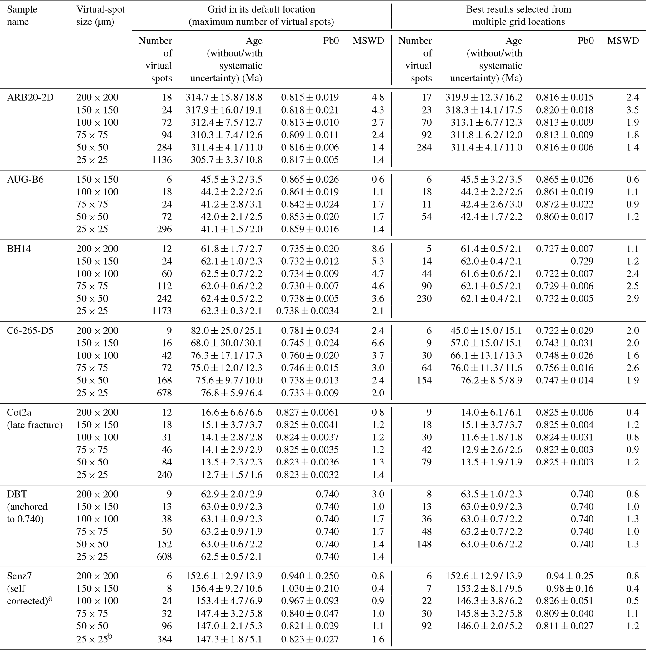
Table 3 Age and common Pb values obtained with the mobile-grid method, for different virtual-spot sizes, using the TW regression. The results presented are those obtained with the default grid position and those corresponding to the best results in terms of precision and MSWD.

^a Based on 50 µm×50 µm virtual spots. ^b One ellipse removed.

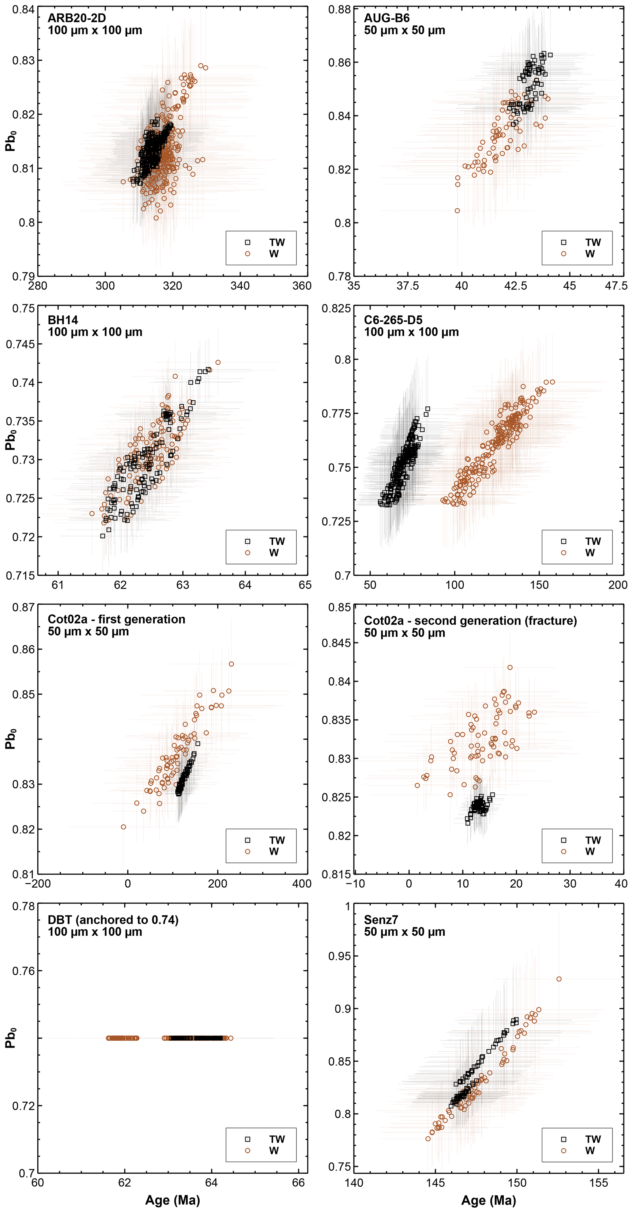
Figure 3 Diagrams showing the ages and common Pb values calculated using the mobile-grid method, based on TW (in black) and W (in brown) regressions, for all samples. For each sample, the results from all grid positions are shown. The error bars are at 95 % confidence level.

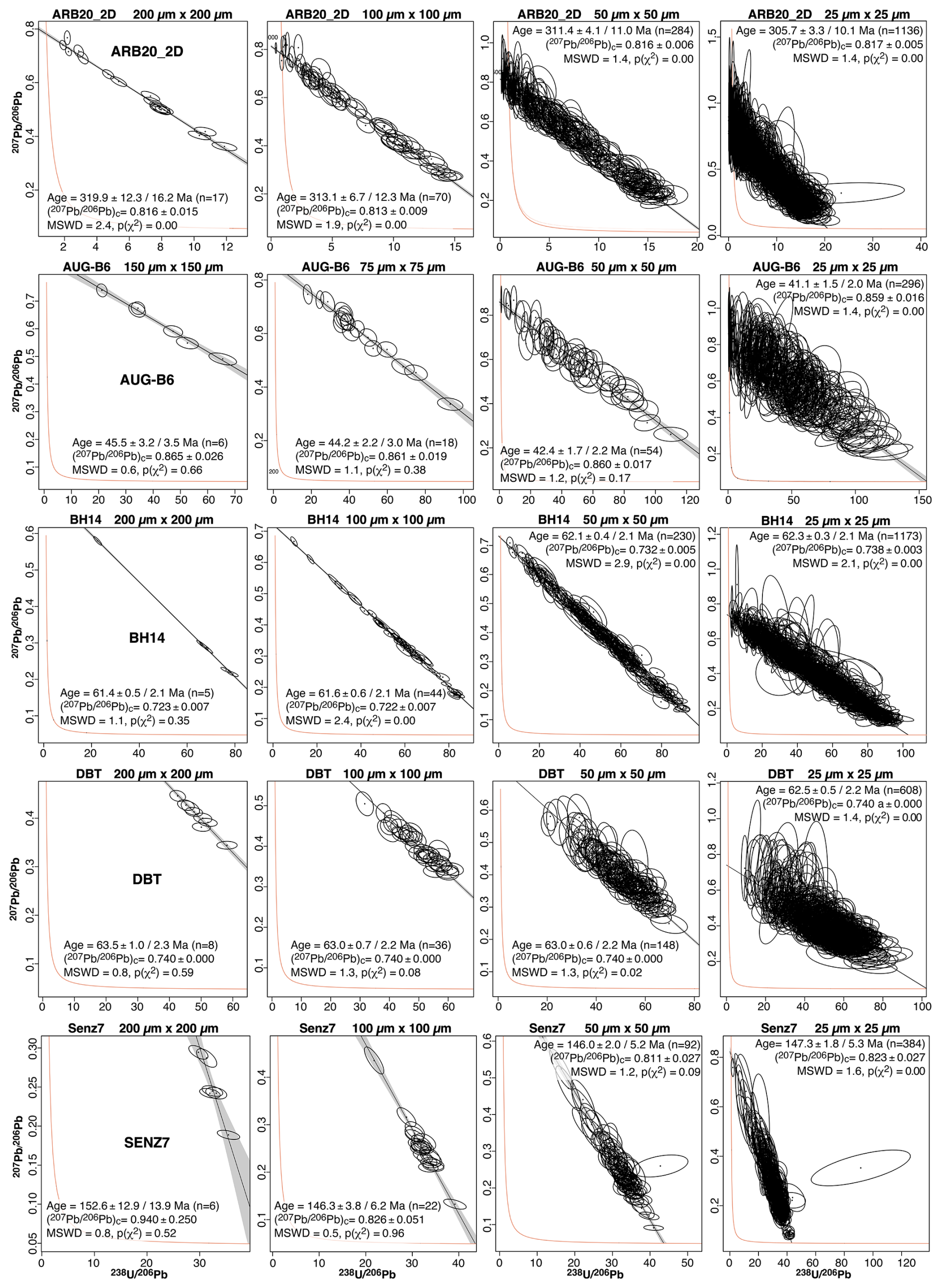
Figure 4 TW diagrams obtained for five samples (ARB20-2D, AUB-B6, BH14, DBT, and Senz7 from top to bottom) for spot sizes of 200 µm×200 µm, 100 µm×100 µm, 50 µm×50 µm, and 25 µm×25 µm (except sample AUG-B6: 150 µm×150 µm, 75 µm×75 µm, 50 µm×50 µm, and 25 µm×25 µm). The diagrams correspond to the grid positions giving the best results in terms of precision and MSWD.

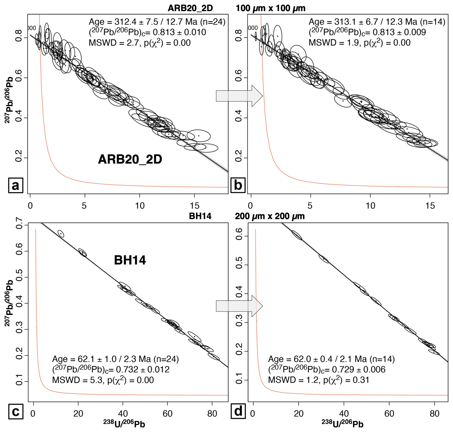
Figure 5 Examples of TW diagrams obtained for ARB20-2D and BH14 with the default grid position (a, c) and those corresponding to the best results in terms of precision and MSWD (b, d).

5.1.2 Case of low-U sample

In the case of samples with low U (and Pb) contents (C6-265-D5), the ages calculated from isotopic maps are clearly biased. First, for 200 and 150 µm spots, the uncertainties of the ages obtained with the TW and W regressions are high (higher than 15 Ma without propagation; Fig. 4, Table 3), and the ages vary widely (from 0 to >200 Ma). For W regressions, they correspond to errorchrons in nearly all grid positions. For lower spot sizes, the ages obtained are not identical in the uncertainties (Fig. 3) and vary according to the spot size. They are much lower in the case of TW regressions than in that of W ones (Figs. 3 and 6a). The ages calculated by TW regression are centered around ∼52–85 Ma (100 µm spots) and ∼67–86 Ma (50 µm spots). W regression results in ages centered around ∼93–155 Ma (100 µm spots) and ∼93–119 Ma (50 µm spots) (Figs. 3 and 6c). These biased values are clearly related to the low number of counts in U and Pb, which induces a large dispersion of isotope ratios (Fig. S2 in the Zenodo repository). They mostly result in high MSWD values. These inconsistencies are resolved by averaging the number of mass sweeps on the time-resolved signal before data processing (equivalent to averaging the number of pixels along each linear scan), as done by Drost et al. (2018) and Hoareau et al. (2021) (Fig. 6b). As shown in Fig. 6c, the mean TW and W ages evolve as a function of the number of averaged pixels, reaching identical values in their uncertainties from a value of 2 and a more restricted range from a value of 3. We note that the calculated average values vary slightly depending on the chosen spot size (∼110–120 Ma for 100 µm and ∼100–110 Ma for 50 µm). Despite their high uncertainties, these ages are consistent with the geological evidence of precipitation in the interval between ∼112 and ∼101 Ma (Pyrenean rifting; Motte et al., 2021). However, it is not possible to definitely ensure that the obtained ages truly reflect the precipitation age of the analyzed dolomite. Therefore, it is necessary to test pixel averaging on samples that yield results similar to those of C6-265-D5 (i.e., differing ages depending on the concordia diagram used, due to low U and/or Pb concentrations) but for which the precipitation age is independently known from other methods.

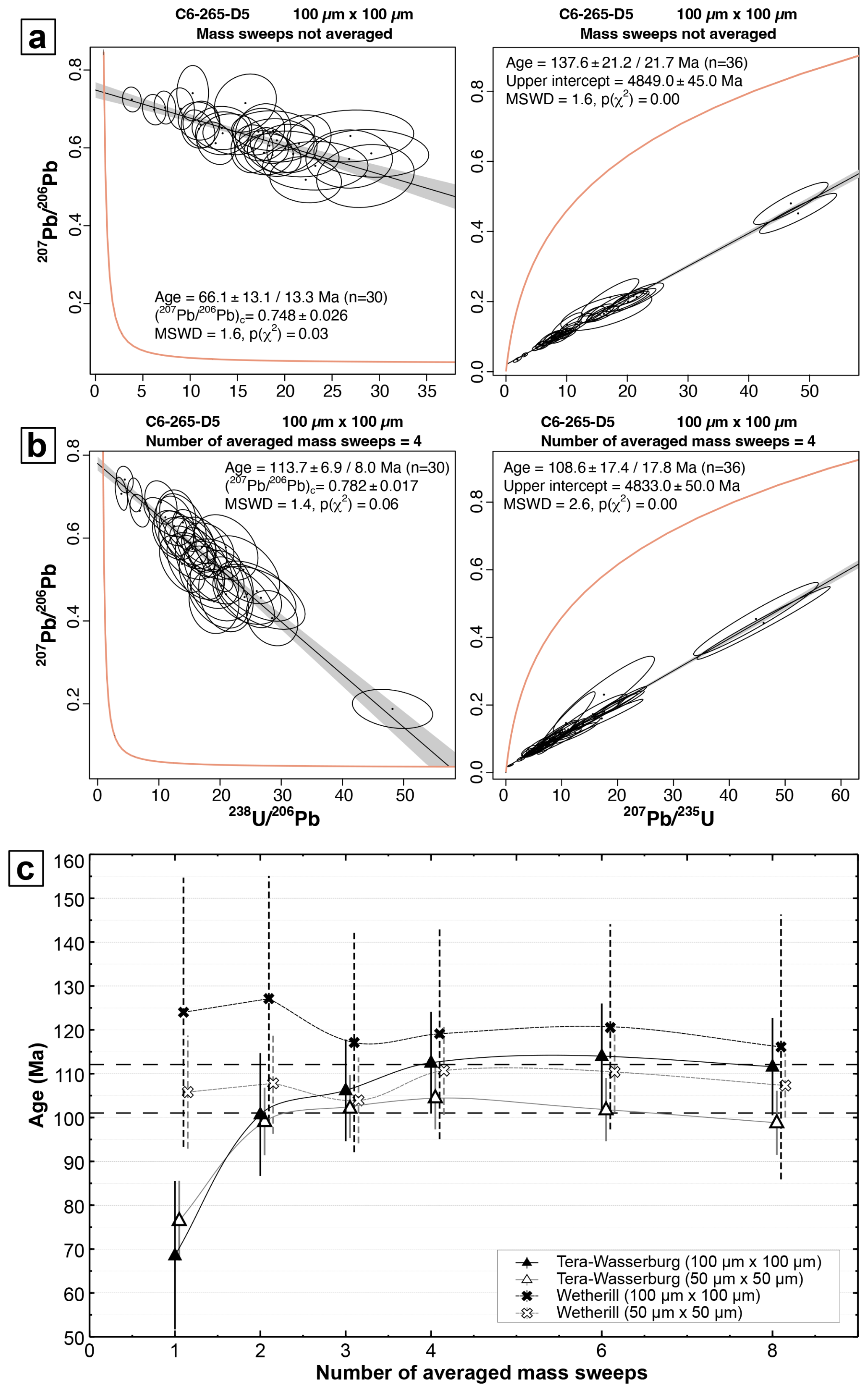
Figure 6 (a) Best age results obtained for the C6-265-D5 sample, with virtual-spot sizes of 100 µm×100 µm and no mass sweep averaging (left: TW diagram; right: W diagram). (b) Same as panel (a) but with four averaged mass sweeps. (c) Evolution of the weighted mean age calculated from several grid positions and for several virtual-spot sizes (50 µm×50 µm and 100 µm×100 µm), as a function of the number of averaged mass sweeps, for sample C6-265-D5. The vertical bars correspond to 95 % standard deviation. The expected age is between 101 and 112 Ma (dashed lines).

5.2 Ages calculated with the Rectis method

Using the Rectis method as a complement to the mobile-grid method also yields very satisfactory results for high-U samples. In accordance with the theory for a sample of homogeneous age, the representation of all possible ellipses in a TW diagram defines a linear trend, with MSWD values close to or below 1 (Figs. 7b and S5 in the Zenodo repository). The ages obtained by orthogonal regression through the set of virtual spots are identical to the expected ones. After selecting the maximum number of non-adjacent 100 or 50 µm spots on an map (starting from the 50 % spots closest to the regression line), expected ages are also obtained with IsoplotR. For several samples (ARB20-2D, BH14, DBT, Senz7), besides the low MSWD values, the age uncertainties are better than those obtained by the mobile-grid method (Fig. 7c; Table 4). For AUG_B6 and Cot02a samples, however, they are higher. In these cases, the virtual spots selected by Rectis may correspond to less spread ellipses in a TW diagram and/or greater individual uncertainties. Regarding C6-265-D5, a similar behavior to that observed with the grid method is obtained. The orthogonal regression gives an age of 72.6 Ma in the TW diagram, with a high MSWD (2.8) indicating the poor alignment of all ellipses (Fig. 7c). The corresponding age after selecting the virtual spots is 68.6 ± 9.8 Ma. With a W diagram, the ages are much higher (126.9 Ma for orthogonal regression and 126.1 ± 17.1 Ma after selection). Averaging the number of mass sweeps by four results in final ages of 120.3 ± 14.3 Ma and 112.3 ± 14.3 Ma (TW and W diagrams, respectively), values that are in better accordance with the expected age, while being associated with lower MSWD values (Fig. 7d). It should be noted that in this case the uncertainties are also lower than those obtained using the mobile-grid method. Once again, the age obtained for C6-265-D5 is consistent with geological constraints (Motte et al., 2021), but it needs to be confirmed using other dating methods, such as isotope dilution.

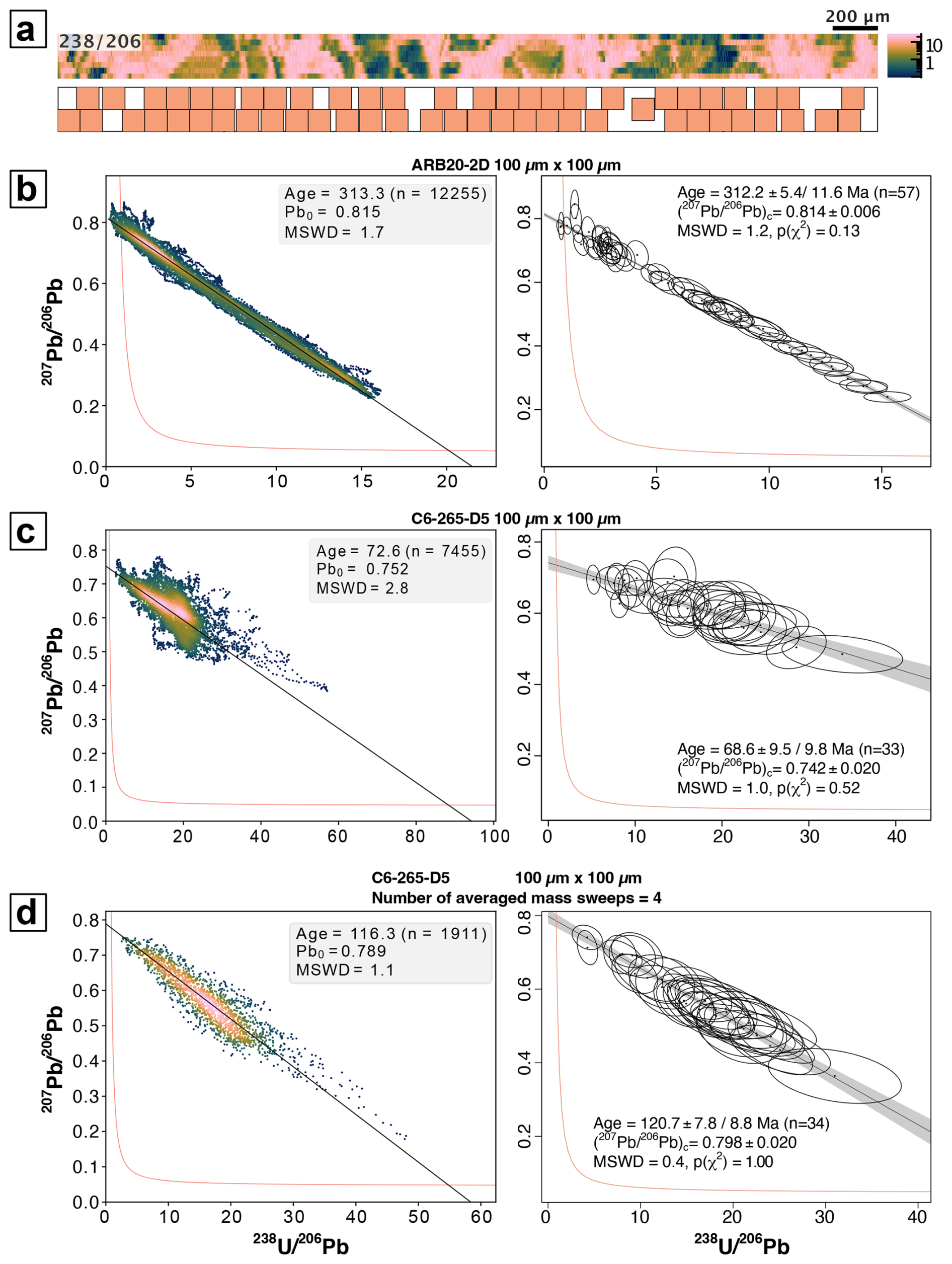
Figure 7 (a) ${}^{\mathrm{238}}\mathrm{U}{/}^{\mathrm{206}}\mathrm{Pb}$ map of ARB20-2D and location of the maximum number of non-adjacent 100 µm×100 µm spots as calculated with the Rectis method. (b) Results obtained for the ARB20-2D sample. Left: TW diagram built from all possible 100 µm×100 µm virtual-spot positions on the map (uncertainties not represented). Age, common Pb, and MSWD values are calculated from Scipy ODR regression. Right: age result obtained from the maximum number of non-adjacent spots using the Rectis method, starting from the 50 % spots closest to the ODR regression line. (c) Same as panel (b) but for the C6-265-D5 sample. (d) Same as panel (c) but with four averaged mass sweeps. See text for details.

Table 4 Age and common Pb values obtained with the Rectis method, using the TW regression. The results presented are those obtained by orthogonal regression (ODR) across all possible virtual spots and after selecting the maximum number of non-adjacent spots on an map. ^a Uncertainties greater than 20 % filtered out; ^b based on 50 µm×50 µm virtual spots.

5.3 Calculation of ages from very small areas

5.3.1 Manual selection of cement phases (Cot02a)

The isotopic mapping obtained on sample Cot02a suggests the presence of several generations of calcite in addition to detrital quartz grains (Fig. 8a). In particular, U and Th concentration maps highlight two distinct calcite generations carrying the highest $\mathrm{U}/\mathrm{Pb}$ ratios, which were manually selected using Iolite4 (Fig. 8a). The first phase (Cal1) consists of two grains adjacent to quartz, covering a total area of approximately 0.064 mm² (equivalent to ∼6 static spots of 100 µm in diameter), or ∼2200 pixels. The average U content is 1.5 ± 0.03 ppm. The second cement phase (Cal2) fills a late fracture about 50 µm wide, cutting across the previous phases as well as the quartz. The total selected area is approximately 0.092 mm² (i.e., ∼9 static spots of 100 µm in diameter), or ∼3800 pixels. U contents are high, with an average value of 6.9 ± 0.2 ppm.

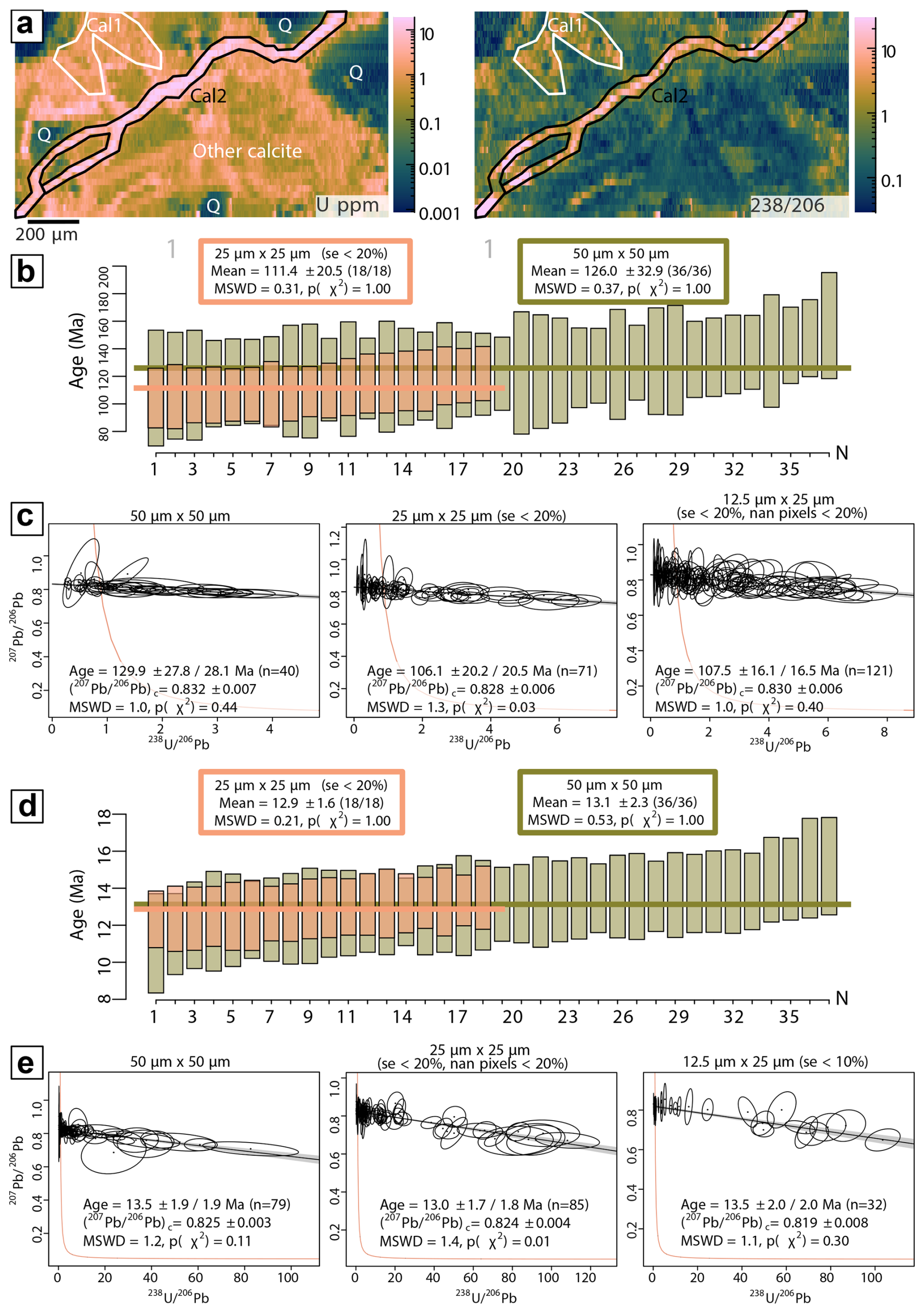
Figure 8 (a) LA-ICP-MS maps of U concentrations (in ppm) and ${}^{\mathrm{238}}\mathrm{U}{/}^{\mathrm{206}}\mathrm{Pb}$ ratios of sample Cot02a. The area highlighted in white (Cal1) corresponds to the first generation of calcite, while the area highlighted in black (Cal2) corresponds to the second. Q: quartz; other calcite: calcite with ${}^{\mathrm{238}}\mathrm{U}{/}^{\mathrm{206}}\mathrm{Pb}$ values too low to be datable. (b) Weighted average of TW ages obtained for the first generation, for different grid positions and virtual-spot sizes. In blue, spots with uncertainties greater than 20 % have been filtered out. (c) Best TW age results obtained for different virtual-spot sizes, for the first generation. For 25 µm spots, spots with more than 20 % of pixels outside the selected area (see Fig. 8a) are excluded, in addition to uncertainties greater than 20 %. For 12.5 µm×25 µm spots, the filtering is based on uncertainties greater than 10 %. (d) Same as panel (b) but for the second generation. (e) Same as panel (c) but for the second generation. For 25 µm spots, spots with more than 20 % of pixels outside the selected area and uncertainties greater than 20 % are filtered out, while for 12.5 µm×25 µm spots, spots with uncertainties greater than 10 % are excluded.

For the first phase, the ${}^{\mathrm{238}}\mathrm{U}{/}^{\mathrm{206}}\mathrm{Pb}$ ratios are very low, resulting in very high uncertainties in the calculated TW ages (∼25–40 Ma for ages centered around ∼110–140 Ma, for virtual spots of 50 µm) (Fig. 8b). As previously described for other samples, W ages are more scattered than TW ages and also present higher individual uncertainties (Fig. 3). While most W ages are similar to TW ages when considering these uncertainties, the presence of errorchrons confirms that dating this generation remains a challenge. As before, reducing the size of the virtual spots and therefore increasing their number helps decrease the age uncertainty, which nevertheless remains above 15 Ma for 25 µm spots (TW diagrams). Since virtual spots may only partially overlap the selected areas, the number of spots may exceed what is expected based on the ratio between the selected cement surface area and the virtual-spot area. Thus, it is possible to obtain up to 135 spots or 270 spots of 25 µm×25 µm or 12.5 µm×25 µm, respectively, on the selected surface, but with individual uncertainties in the ${}^{\mathrm{238}}\mathrm{U}{/}^{\mathrm{206}}\mathrm{Pb}$ and ${}^{\mathrm{207}}\mathrm{Pb}{/}^{\mathrm{206}}\mathrm{Pb}$ ratios that can sometimes exceed 50 %. Filtering out uncertainties above 20 % (as example) reduces the final number of spots but allows obtaining close age values regardless of the position of the virtual grid (∼90–110 ± 20 Ma) (Fig. 8b and c). Additionally, filtering out spots containing too many pixels outside the selected zone (i.e., spots partially overflowing from this zone and thus with a high number of unused pixels) results in close results, but with MSWD values closer to unity (Fig. 8c). Due to low ${}^{\mathrm{238}}\mathrm{U}{/}^{\mathrm{206}}\mathrm{Pb}$ values, such ages are roughly consistent with the stratigraphic age of the host carbonate (Coniacian-Santonian, i.e., 90–84 Ma). However, a more precise TW age of 83.0 ± 7.5 Ma was obtained from similar grains from another map made on the same sample (Fig. S6 in the Zenodo repository), suggesting that in fact depositional carbonate or early calcite cement may have been remobilized by the shear band formed during the Pyrenean orogeny.

For the second cement phase, a similar methodology yields much more recent TW ages (∼12–14 Ma), in accordance with the petrographic evidence of late-stage fracturing (Fig. 8d). Once again, W ages exhibit significantly greater dispersion and lower precision compared to TW ages, which are preferred (Fig. 3). It is interesting to note that for very small spot sizes (e.g., 12.5 µm×25 µm), filtering out spots with uncertainties in the ratios above, for example, 10 %, logically reduces the number of spots significantly (from 436 to 32) but provides TW age uncertainties around 2 Ma, which are generally comparable to those obtained when all spots are retained (Fig. 8e). This allows testing various configurations (virtual-spot sizes, filtering or not, grid migration) to find the parameters that yield the most reliable ages possible.

5.3.2 Micro-maps (sub-map method) and weighted average of ages

Here we use the example of samples ARB20-2D and BH14, which are highly suitable for dating due to their high U content and good spread of ratio values, to demonstrate the possibility of obtaining ages from isotopic mapping of extremely small surfaces, comparable to that of a single spot in the conventional LA-ICP-MS approach, and of calculating weighted mean ages for a larger map. The isotopic map obtained on ARB20-2D covers an area of ∼0.72 mm² (20 488 pixels), which corresponds to 18, 72, 290, and 1160 virtual spots of 200, 100, 50, and 25 µm on each side, respectively. By choosing a 25 µm grid, the map can then be divided, for example, into 18 sub-maps of 200 µm×200 µm, each containing 64 virtual spots of 25 µm×25 µm, or into 72 sub-maps of 100 µm×100 µm, each containing 16 virtual spots (Fig. 9a). In the case of 200 µm sub-maps, the TW ages calculated for each sub-map are mostly comparable to the age obtained from the entire map using 25 µm spots (∼305.7 ± 3.3 / 8.7 Ma) within the limits of uncertainties, with uncertainties that can be below 10 %. The weighted mean age (306.6 ± 3.1 Ma without propagated uncertainties) is also identical to the expected age (Fig. 9b). The precision of the ages can be improved by choosing even smaller spot sizes (12.5 µm×25 µm), corresponding to 128 virtual spots per 200 µm×200 µm sub-map (Fig. 9c). In this case, 90 % of the ages have uncertainties below 10 %, with a comparable weighted mean (300.0 ± 3.1 Ma). Additionally, choosing 50 µm virtual spots provides greater accuracy in the calculated ages. In the case of 100 µm sub-maps, the obtained TW ages have higher uncertainties, but the weighted mean is close (307.0 ± 3.4 Ma and 301.1 ± 3.2 Ma for 25 µm×25 µm and 12.5 µm×25 µm spots, respectively; Fig. 9b). However, it should be noted that in all cases, several ages from the sub-maps differ from the expected age within the limits of uncertainties. By following the same procedure for sample BH14, the obtained ages for most sub-maps are mostly identical to the expected age, with uncertainties generally better than 10 % (Fig. 10). The weighted means are also perfectly comparable to the expected age. Again, choosing 50 µm spots in 200 µm sub-maps yields the most reliable results (all ages are comparable to the expected age). In conclusion, these examples show that for favorable samples (U>1 ppm, variable $\mathrm{U}/\mathrm{Pb}$), dating from 100 or 200 µm maps is possible, with slightly lower precision and, to a lesser extent, accuracy compared to more conventional approaches. The calculation of weighted mean ages also allows controlling the quality of the age obtained from the isotopic maps.

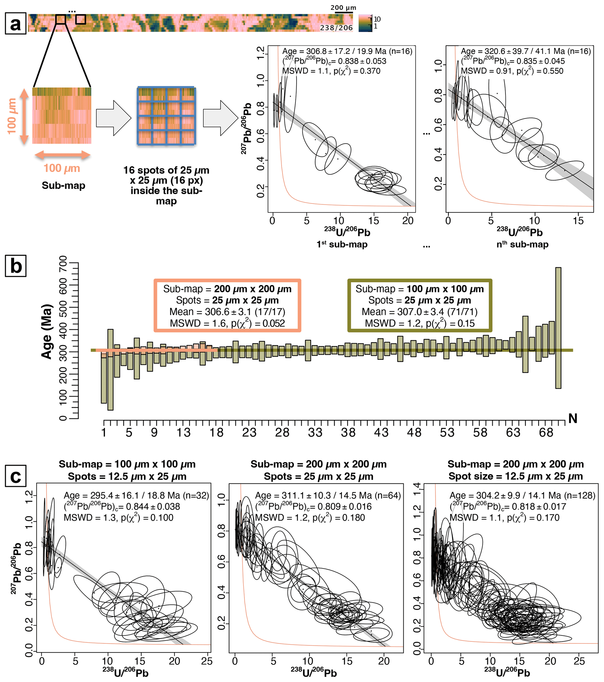
Figure 9 (a) Scheme illustrating the procedure used to obtain ages from sub-maps, based on the ARB20-2D sample. A 100 µm×100 µm (or 200 µm×200 µm) map is extracted from the initial isotope map. It is itself discretized into small virtual spots (typically 25 µm×25 µm). Two TW diagrams obtained from two different sub-maps are shown as examples. (b) Weighted averages of TW ages obtained from different sub-maps for ARB20-2D, for 25 µm×25 µm virtual spots. The 200 µm sub-maps are shown in blue, and the 100 µm sub-maps are shown in green. Systematic uncertainties are not considered. (c) TW diagrams of the best results obtained for different sub-map and virtual-spot sizes. Note the good distribution of ellipses despite the small size of the sub-maps and the similarity of the calculated ages.

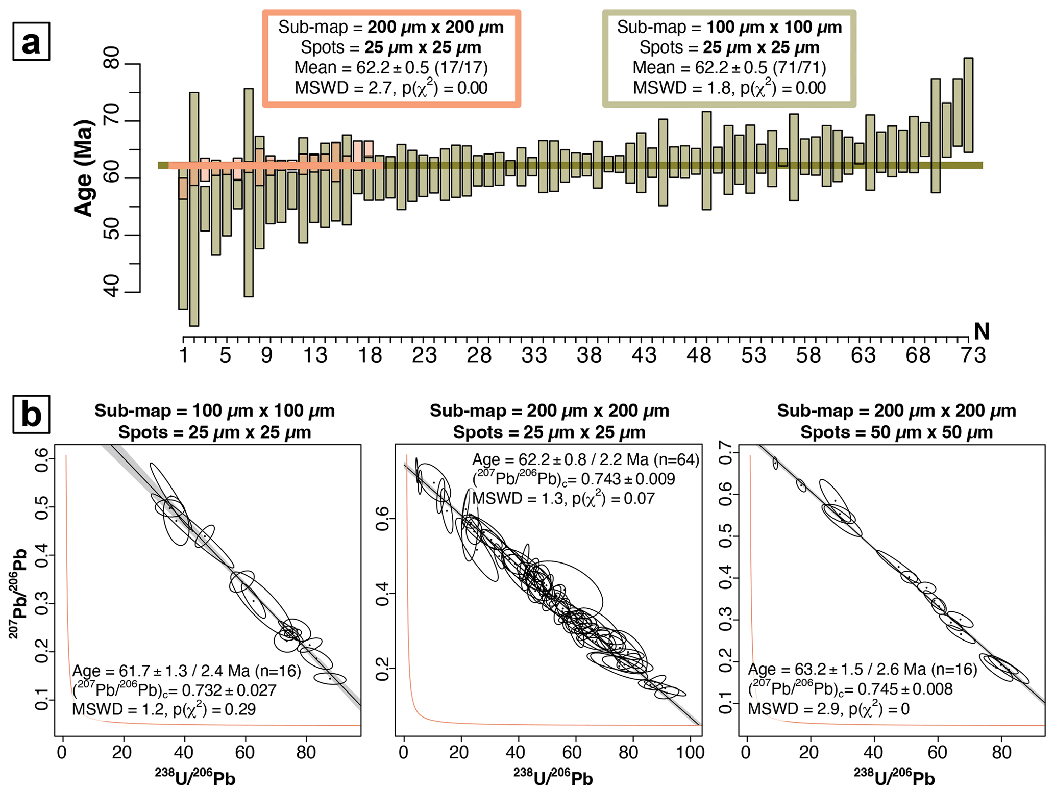
Figure 10 (a) Weighted averages of TW ages obtained from different sub-maps for BH14, for 25 µm×25 µm virtual spots. The 200 µm sub-maps are shown in blue, and the 100 µm sub-maps are shown in green. Systematic uncertainties are not considered. (b) TW diagrams of the best results obtained for different sub-map and virtual-spot sizes. Note the good distribution of ellipses despite the small size of the sub-maps and the similarity of the calculated ages.

6 Discussion

6.1 Interest and limitations of the virtual-spot approach

The interest and inherent limitations of extracting ages from isotopic maps by LA-ICP-MS have already been addressed by several authors (Drost et al., 2018; Roberts et al., 2020; Hoareau et al., 2021; Davis and Rochín-Bañaga, 2021; Liu et al., 2023). One of the main advantages of isotopic maps, as detailed by Drost et al. (2018) and Roberts et al. (2020), is the ability to isolate pixels (either individually or as a range) based on their associated compositions or isotopic ratios, for example, to highlight multiple generations of cements or reject pixels with composition anomalies that may indicate detrital contamination before calculating one or more ages. Moreover, it is always possible to isolate ranges using co-localization approaches (Hoareau et al., 2021) or simply by manual selection in suitable software (here, Iolite4; see also Ansberque et al., 2021; Chew et al., 2021). Various data processing methods for age calculations on carbonates have been proposed since the study by Drost et al. (2018). These include the pixel pooling method (Drost et al., 2018), robust regression on the values of the isotopic ratios of interest (Hoareau et al., 2021), and Bayesian regression (Davis and Rochín-Bañaga, 2021; Liu et al., 2023). As already discussed in the introduction, each approach has its advantages and disadvantages, and the present approach is no exception to this rule.

The results presented here show that for samples traditionally favorable for U–Pb dating of carbonates by LA-ICP-MS (U>100 ppb, good spread of $\mathrm{U}/\mathrm{Pb}$ ratios of pixels), the virtual-spot approach has several interesting advantages, especially when used on data obtained with a high-repetition-rate laser that allows high spatial resolutions (here, pixels of 25 µm×1.3 µm), coupled with a high-sensitivity spectrometer (here, an SF-ICP-MS). In fact, it is possible, from isotopic maps typically obtained in less than 1 h, to generate hundreds of virtual spots covering the selected carbonate phases with the mobile-grid method. The ability to adjust the virtual-spot size allows finding the most suitable combination in terms of statistics on the considered cement (low age uncertainty, MSWD close to 1) while avoiding possible accuracy biases through alternative approaches. The example of the Cot6a sample shows that robust ages are obtained on a mineralized fracture less than 50 µm thick, which would have been challenging to date with conventional static spot approaches. Here, the ability to generate more than 100 spots smaller than 50 µm is a notable advantage. Generally, spot sizes of 50 µm×50 µm yield very satisfactory results. Another development presented here is the use of a mobile grid for virtual spots, which allows the user to calculate several tens of ages from the same map to evaluate their relevance, for example, through the visualization of their weighted means. In the case of reliable samples (i.e., with a homogeneous age and common Pb composition, sufficiently high U and Pb concentrations, and a wide enough range in isotopic ratios to allow for both accurate and precise U–Pb dating), it is expected that the position of the spots does not influence the calculated ages. It is then possible to choose the final age with the best statistical parameters. The Rectis method offers an alternative approach to age calculation that can results in even better statistical results. Finally, the approach can allow for age calculation from very small map dimensions (down to 100 µm×100 µm) (sub-map method), although with the limitations presented with the examples of samples ARB20-2D and BH14. For larger maps, dividing them into sub-maps allows the calculation of weighted mean ages, providing an additional way to evaluate the relevance of a cement age.

However, the virtual-spot approach is not flawless. First, the results obtained on sample C6-265-D5 show that a bias towards a too young age is possible when U and/or Pb concentrations are too low. It is then necessary to average the pixels (as done by Drost et al., 2018) and compare the ages obtained on TW and W diagrams to obtain a satisfactory result, which can be laborious. Even with such pixel averaging, tests carried out on the ASH15 standard (Nuriel et al., 2021) failed to obtain a reliable age due to the very low Pb content of the sample (<7 ppb), although this standard is used by several teams equipped with an identical mass spectrometer (e.g., Montano et al., 2021; Guillong et al., 2020). At the end of this study, it remains necessary to test additional samples with low U and Pb concentrations but independently known ages, in order to verify that pixel averaging yields accurate ages. This problem of possible bias also requires further work on the conditions under which LA-ICP-MS maps are acquired, but our tests generally suggest that the comparison between TW and W results should be systematic, including in LA-ICP-MS U–Pb dating using static spots. Second, each virtual spot is obtained from adjacent pixels rather than from the progressive ablation of the same surface as in the case of static spots. Given the variation of isotopic ratio values at the microscopic scale in carbonates, and despite signal mixing resulting from the washout time, it is expected that the uncertainty of the average obtained for each virtual spot will be larger. This limitation can be counterbalanced by using more virtual spots, as shown by the results obtained, for example, on samples BH14, DBT, AUG-B6, and ARB20-2D. Another counterintuitive effect of using virtual spots is the occurrence of high MSWD values for samples particularly favorable for dating, due to high error correlations. Sample BH14 is representative of this effect. For each virtual spot (100 µm×100 µm), the variations in the ${}^{\mathrm{238}}\mathrm{U}{/}^{\mathrm{206}}\mathrm{Pb}$ and ${}^{\mathrm{207}}\mathrm{Pb}{/}^{\mathrm{206}}\mathrm{Pb}$ ratios are significant, resulting in high error correlations. This characteristic is likely to highlight minor heterogeneities in the sample. These indeed seem to exist in sample BH14 as shown by the MSWD value of 4.7 also obtained by Hoareau et al. (2021) with static spots of same size – higher than the value of 1.6 of Beaudoin et al. (2018). Note that this error correlation effect can also be considered an additional means of better characterizing the sample in question in favor of the approach presented here.

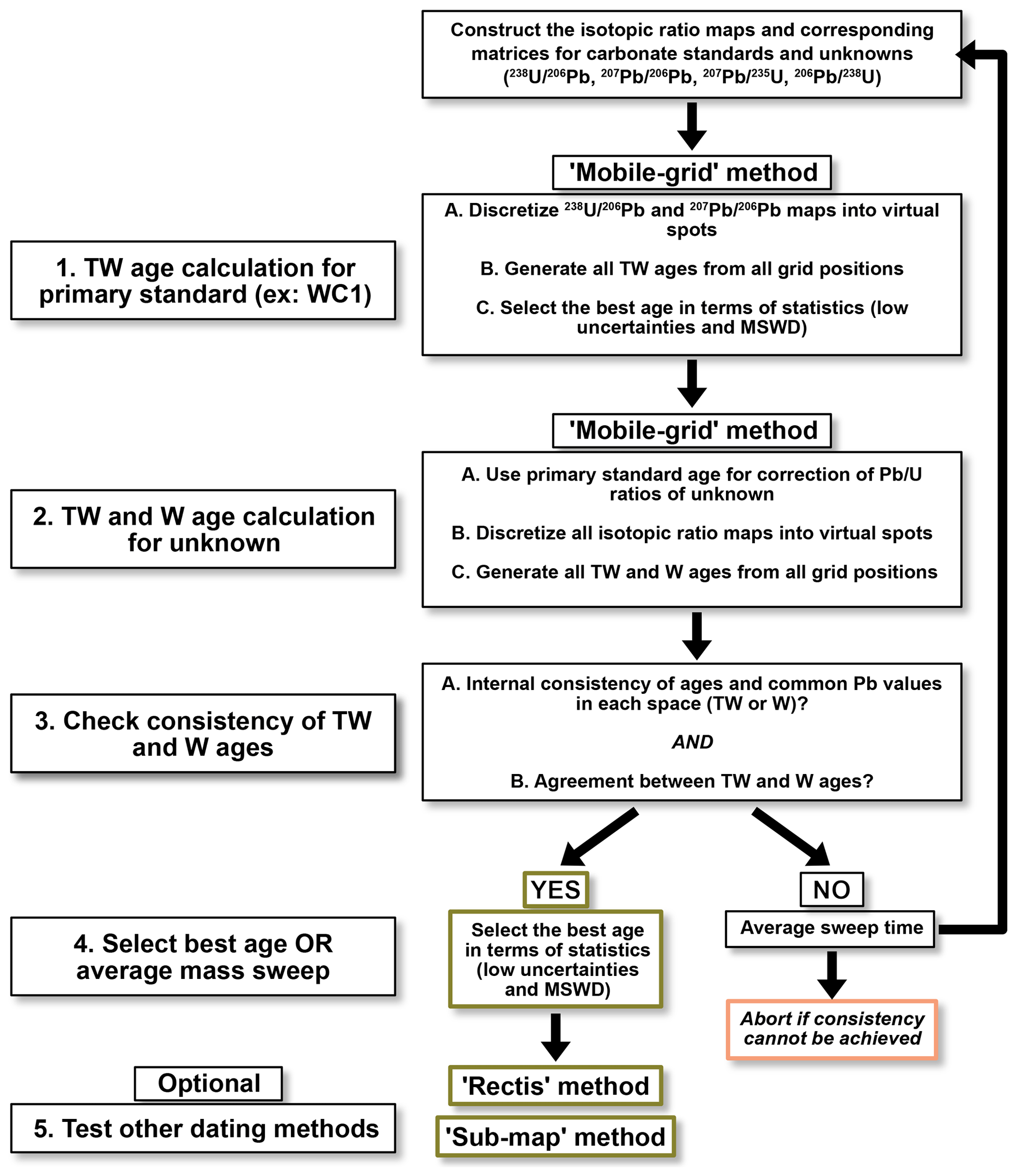
6.2 Guidelines for a proper use of the approach

To use the virtual-spot approach in the most effective and logical way – particularly considering the potential accuracy biases discussed earlier – we propose some guidelines, which are also summarized in Fig. 11. A detailed user guide is provided in the Zenodo repository. At this stage, we assume that the isotopic ratio maps and corresponding matrices of both standards and unknown-age samples have already been constructed using Iolite.

• 1.

  Age calculation for primary standard (mobile grid). The first step is to calculate the uncorrected TW age of the primary standard (here, WC-1). Under the analytical conditions of our study, a virtual-spot size of 50 µm×50 µm or 75 µm×75 µm is appropriate. Thanks to the mobile-grid approach, several dozen ages are generated, and the one with the best statistical parameters can be selected and used for the correction of unknown samples as well as secondary standards.

• 2.

  Age calculation for the unknown sample (mobile grid). As with the primary standard, a series of ages is calculated for the unknown sample using the mobile-grid method. By default, a virtual-spot size of 100 µm×100 µm is used, but other sizes may be chosen. At this stage, it is strongly recommended to perform age calculations in both TW and W concordia spaces.

• 3.

  Check consistency (mobile grid). Assess (i) internal consistency of the age and common Pb values in each space (TW or W) and (ii) agreement between TW and W ages, within uncertainty limits. Both conditions must be satisfied. If not, one may investigate the potential causes (e.g., low $\mathrm{U}/\mathrm{Pb}$ concentrations, insufficient isotopic ratio spread, multiple age populations).

• 4.

  Selection of final age (mobile grid) or mass sweep averaging.

  • 4a.

    If the ages are consistent, select the most statistically robust result (e.g., lowest MSWD, highest precision), potentially adjusting the virtual-spot size to improve the results, and add external uncertainty onto the final age.

  • 4b.

    If the TW and W ages are inconsistent (as for C6-265-D5), recalculate the ages from the beginning after averaging the mass scans. If the TW and W results now converge, return to step 4a. If not, the sample is likely undatable.

• 5.

  Optional steps (provided step 4 is successful).

  • 5a.

    Apply the Rectis method to obtain a potentially more precise age or one with better statistical parameters.

  • 5b.

    Use the sub-map method as an additional test. The weighted mean of the sub-map ages should ideally match the result obtained using the mobile-grid method. Note that this method is expected to give satisfactory results only for appropriate samples (high U content and good spread of ratio values).

Figure 11 Guidelines for a proper use of the virtual-spot approach.

6.3 Further developments

Further developments can be envisaged for the virtual-spot method to further enhance its appeal. A first major development will be to propose a routine that automatically selects virtual spots for maximum spread of isotope ratio values, for the number of virtual spots chosen by the user. This should lead to improved accuracy and precision of calculated ages. Other developments could include the automatic definition of virtual spots of variable size and shape, depending on the precision of the resulting isotope ratios, with a view to improving age calculations. Finally, in a more fundamental sense, the use of an average and its uncertainty implies that the distribution of pixel isotopic ratio values follows a normal distribution for each spot, which is probably valid only for the largest spots due to their higher number of pixels. The similarity and accuracy of the ages obtained here for different virtual-spot sizes shows that the skewed pixel value distribution does not introduce measurable bias into the results. However, additional tests must focus on using alternative statistics such as the median and its uncertainty.

7 Conclusion

The U–Pb carbonate dating approach from isotopic maps presented here benefits from the use of a high-sensitivity ICP-SF-MS coupled with a high-repetition-rate femtosecond ablation laser. The high ablation rate (>100 Hz) enables the construction of maps from lines of only 25 µm width. The maps are then simply separated into a grid of virtual spots for the calculation of ages. Tests carried out on samples of known age show that the ages obtained correspond to reliable ages unbiased by the processing method. For samples with low U concentrations and noisy $\mathrm{U}/\mathrm{Pb}$ and $\mathrm{Pb}/\mathrm{Pb}$ ratios, comparison of the ages obtained from the TW and W diagrams, together with smoothing of the number of pixels in the isotopic maps, seems to correct the bias towards inaccurate ages obtained from the unsmoothed maps. In addition to the advantages inherent to the use of isotopic maps described elsewhere (such as the possibility of filtering pixels or manually selecting regions of interest), the ability to move virtual-spot grids implies that several ages can be obtained for the same study area, helping to assess their homogeneity. Finally, in the case of U-rich samples, we show that one can obtain reliable ages from very small maps (<0.04 mm²), paving the way for dating samples traditionally inaccessible to geochronology, such as micro-veins or micro-fossils. Although only tested on carbonates, there are no a priori limitations to the use of the virtual-spot approach on other minerals traditionally used in U–Pb geochronology.

Appendix A

Table A1 Analytical conditions.