Seasonal deposition processes and chronology of a varved Holocene lake sediment record from Chatyr Kol lake (Kyrgyz Republic)

Microfacies analysis of a sediment record from Chatyr Kol lake (Kyrgyz Republic) reveals the presence of seasonal laminae (varves) from the sediment base dated at 11 619±603 BP (years Before Present) up to $\sim \mathrm{360}\pm \mathrm{40}$ BP. The Chatvd19 floating varve chronology relies on replicate varve counts on overlapping petrographic thin sections with an uncertainty of ±5 %. The uppermost non-varved interval was chronologically constrained by ²¹⁰Pb and ¹³⁷Cs gamma spectrometry and interpolation based on varve thickness measurements of adjacent varved intervals with an assumed maximum uncertainty of 10 %. Six varve types were distinguished, are described in detail, and show a changing predominance of clastic-organic, clastic-calcitic or clastic-aragonitic, calcitic-clastic, organic-clastic, and clastic-diatom varves throughout the Holocene. Variations in varve thickness and the number and composition of seasonal sublayers are attributed to (1) changes in the amount of summer or winter/spring precipitation affecting local runoff and erosion and/or to (2) evaporative conditions during summer. Radiocarbon dating of bulk organic matter, daphnia remains, aquatic plant remains, and Ruppia maritima seeds reveals reservoir ages with a clear decreasing trend up core from ∼6150 years in the early Holocene, to ∼3000 years in the mid-Holocene, to ∼1000 years and less in the late Holocene and modern times. In contrast, two radiocarbon dates from terrestrial plant remains are in good agreement with the varve-based chronology.

1 Introduction

The interplay of the large atmospheric circulation systems in Central Asia (CA), including the Siberian High, the westerlies, and the Indian Monsoon, and their influences on regional climate are still not fully understood. This is partly due to the large contrasts of landscapes (high mountains, deep basins, large water bodies, and deserts), the low spatial and temporal coverage of high-resolution palaeoclimate archives, and the partly problematic dating of these archives in this area. Information about Holocene climate variability in CA derives from several types of archives, including tree rings (Esper et al., 2003), speleothems (Fohlmeister et al., 2017; Wolff et al., 2017), ice cores (Aizen, 2004), aeolian deposits (Huayu et al., 2010), and lakes (Heinecke et al., 2017; Lauterbach et al., 2014; Mathis et al., 2014; Rasmussen et al., 2000; Ricketts et al., 2001; Schwarz et al., 2017). However, none of these lake records have reported annually laminated sediments. In Kyrgyzstan, varves have only been reported from Sary Chelek lake for the short time interval from ∼1940s to 2013 (Lauterbach et al., 2019). Other varved records in the wider region are from Telmen Lake in northern Mongolia, which includes discontinuous varved intervals during the last ca. 4390 cal BP (Peck et al., 2002) and from Sugan Lake in northwestern China covering the last ∼2670 BP (Zhou et al., 2007). Deciphering Holocene climate changes based on limnic records in CA is challenging due to the influences of several factors: (1) chronological uncertainties caused by the scarcity of datable terrestrial plant material at high altitudes and often large ¹⁴C reservoir effects of aquatic organic material (Hou et al., 2012; Lockot et al., 2016; Mischke et al., 2013); (2) human influence (Boomer et al., 2000; Mathis et al., 2014), possibly overprinting the natural climate signals in the archives; and (3) variations in the dominance of the mid-latitude westerlies, the Siberian High, and the Asian Monsoon system leading to different spatial and temporal climate effects over CA (Chen et al., 2008; Herzschuh, 2006; Mischke et al., 2017; Schroeter et al., 2020). All these factors can hamper data comparison and may lead to different palaeoenvironmental interpretations (Chen et al., 2008; Hou et al., 2012; Mischke et al., 2017). The investigation of varved lake sediments offers the unique opportunity for independent dating through varve counting. In addition, the description of varve micro-facies has the potential to provide detailed insights into environmental and climate variations at a seasonal scale. The sediment record from Chatyr Kol lake is the first varved record from CA covering most of the Holocene and the main goal of this study is to establish a robust age model through an integrated dating approach primarily based on varve counting. Varve counting requires an in-depth understanding of seasonal deposition of all varve types occurring in the sediment record. Therefore, we apply continuous micro-facies analysis for the entire sediment profile to describe the Holocene evolution of varve formation in detail and discuss fundamental deposition processes.

2 Study site

Chatyr Kol lake ($\mathrm{40}{}^{\circ }{\mathrm{36}}^{\prime }$ N, $\mathrm{75}{}^{\circ }{\mathrm{14}}^{\prime }$ E) (Fig. 1) is located at ∼3530 m above sea level (a.s.l.) in the intramontane Aksai Basin (De Grave et al., 2011; Koppes et al., 2008) in the southern Kyrgyz Republic. In the north, the basin is restricted by the At-Bashy Range and in the south by the Torugat mountain range, resulting in a catchment area of about 1084 km². Geologically, the surrounding mountain ranges belong to Silurian to Carboniferous sedimentary-volcanogenic complexes of marine–continental collision zones, consisting of limestones and dolomites, that crop out directly along the northern lakeshore, as well as siliceous rocks, shales, and scattered Permian granites that crop out in the south and north-east (Academy of Science of the Kyrgyz SSR, 1987). The modern lake, which has a maximum length of 23 km, a width of 10 km, and a maximum depth of 20 m in its western-central part, is endorheic and separated from the neighbouring Arpa river basin in the north-west by a moraine (Shnitnikov et al., 1978). The moraine originates from glacial advances of unknown age from the western Torugat mountain range. Present-day glaciers exist above ∼4000 m a.s.l. on the Torugat and At-Bashy mountain ranges, but only some of the At-Bashy glaciers drain into Chatyr Kol via the Kegagyr River. The lake further receives convective rainfall in summer (Aizen et al., 2001). A shallow dam at ∼3550 m a.s.l. hinders outflow to the east. Modern climate conditions are generally dry and mainly controlled by the westerlies and the Siberian Anticyclone Circulation (Aizen et al., 2001; Koppes et al., 2008). Mean annual precipitation is ∼275 mm yr⁻¹ as indicated by Aizen et al. (2001) for the evaluation and spatial averaging of annual precipitation of historical records published by Hydrometeo Publishing (Reference Book of Climate USSR, Kyrgyz SSR, 1988). This is comparable to long-term instrumental data from nearby (about 50 km away) weather stations at comparable altitudes, where annual precipitation means are 237 mm yr⁻¹ (station Chatirkul; $\mathrm{40}{}^{\circ }{\mathrm{6}}^{\prime }$ N, $\mathrm{75}{}^{\circ }{\mathrm{8}}^{\prime }$ E; 3540 m a.s.l, 1961–1990 CE) and 294 mm yr⁻¹ (station Tian Shan; $\mathrm{41}{}^{\circ }{\mathrm{9}}^{\prime }$ N, $\mathrm{78}{}^{\circ }{\mathrm{2}}^{\prime }$ E; 3614 m a.s.l., 1930–2000 CE) (Williams and Konovalov, 2008). Monthly-mean temperatures range from −26.0 to 8.0 ^∘C (Koppes et al., 2008; Academy of Science of the Kyrgyz SSR, 1987) with means of −5.4 ^∘C (station Chatirkul) and −7.6 ^∘C (station Tian Shan) (Williams and Konovalov, 2008). The salinity of the lake water ranges from 1.06–1.15 g L⁻¹ in the deeper western part of the lake to 0.24 g L⁻¹ in the shallower eastern part near the inflow (Romanovsky, 2007). Measurements of oxygen concentrations (YSI Pro 6600 V2) during a field trip in July 2012 ranged from ∼6 mg L⁻¹ at the water surface to ∼1 mg L⁻¹ at 19 m depth with a clear oxygen minimum zone below ∼11 m depth (Fig. 2). Water surface and bottom water temperatures (YSI Castaway CTD) at 19 m depth reached 13.2 and 9.4 ^∘C. Specific conductivity (CTD) ranged from 1902 µS cm⁻¹ at 19 m to 1825 µS cm⁻¹; pH was ∼9 (YSI Pro 6600 V2). Secchi depth was about 4 m. Nowadays, the lake is largely occupied by the amphipod Gammarus alius sp. nov. (Sidorov, 2012), and no fish live in the lake (Shnitnikov et al., 1978).

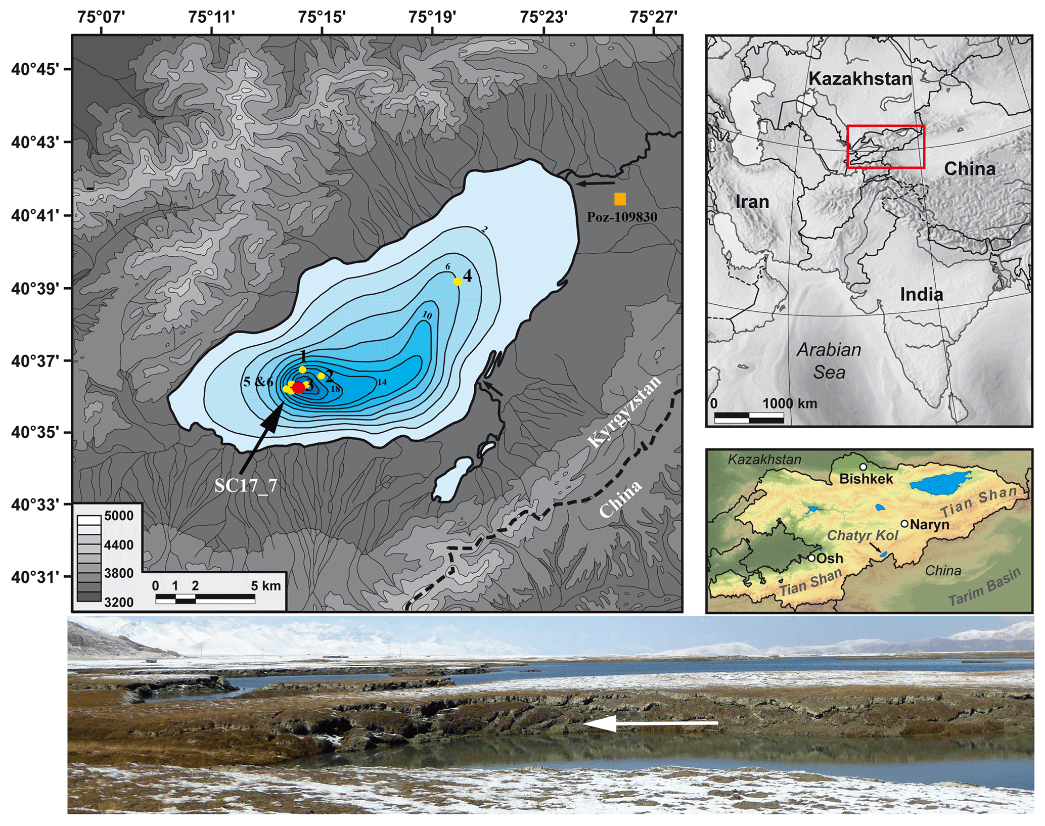
Figure 1 Location of Chatyr Kol lake, the composite profile (red dot), and the gravity cores (yellow dots). The orange square marks the location of ¹⁴C-dated leaves (Poz-109830, Table 2) found in the top of a mid-Holocene shoreline at ∼3540 m a.s.l. The relief map of Kyrgyzstan relies on the CGIAR-CSI SRTM 90 m (3 arcsec) digital elevation data (version 4) of the NASA Shuttle Radar Topography Mission (Jarvis, 2008). The figure was modified from Lauterbach et al. (2014). Photo of unstable shores (white arrow) of Maloye lake.

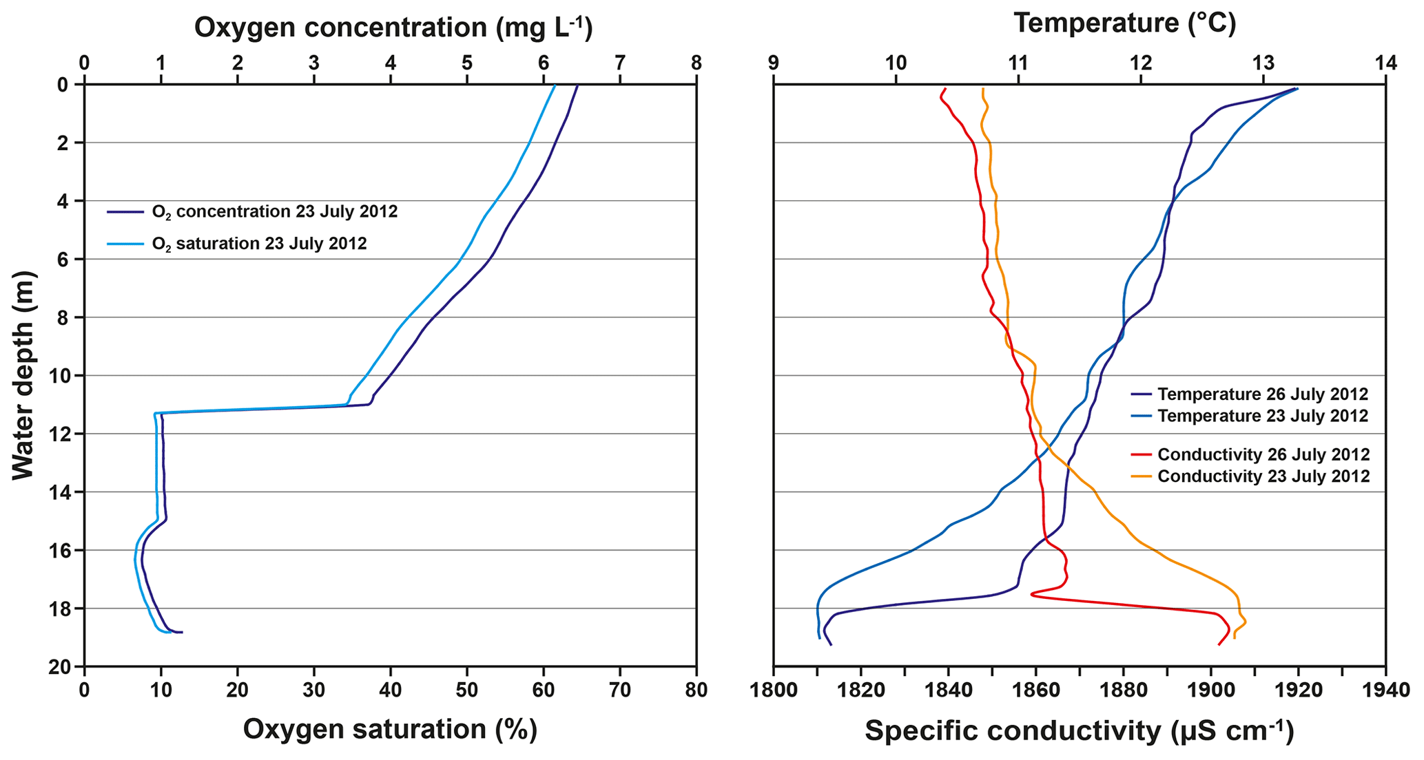
Figure 2 Oxygen concentration (YSI Pro 6600 V2), temperature, and specific conductivity measured with a CTD sensor during the field trip in 2012 at the core's location ($\mathrm{40}{}^{\circ }{\mathrm{36.371}}^{\prime }$ N, $\mathrm{75}{}^{\circ }{\mathrm{14.006}}^{\prime }$ E).

The permafrost level is located at a depth of 2.5–3 m in the littoral coast zones, and the lake is covered by ice from October to April (Shnitnikov et al., 1978). Modern permafrost thawing results in unstable shores visible at the Maloye lake located <2 km to the south of Chatyr Kol (Fig. 1, photo) and the development of small ponds on the shallow south-western shore of this lake and Chatyr Kol lake during summer. Several terraces in the north, south, and east of the lake result from Pleistocene–Holocene lake level fluctuations (Shnitnikov et al., 1978). Vegetation around the lake is generally poor and represented by high alpine meadows (Shnitnikov et al., 1978; Taft et al., 2011).

3 Methods

3.1 Coring and composite profile

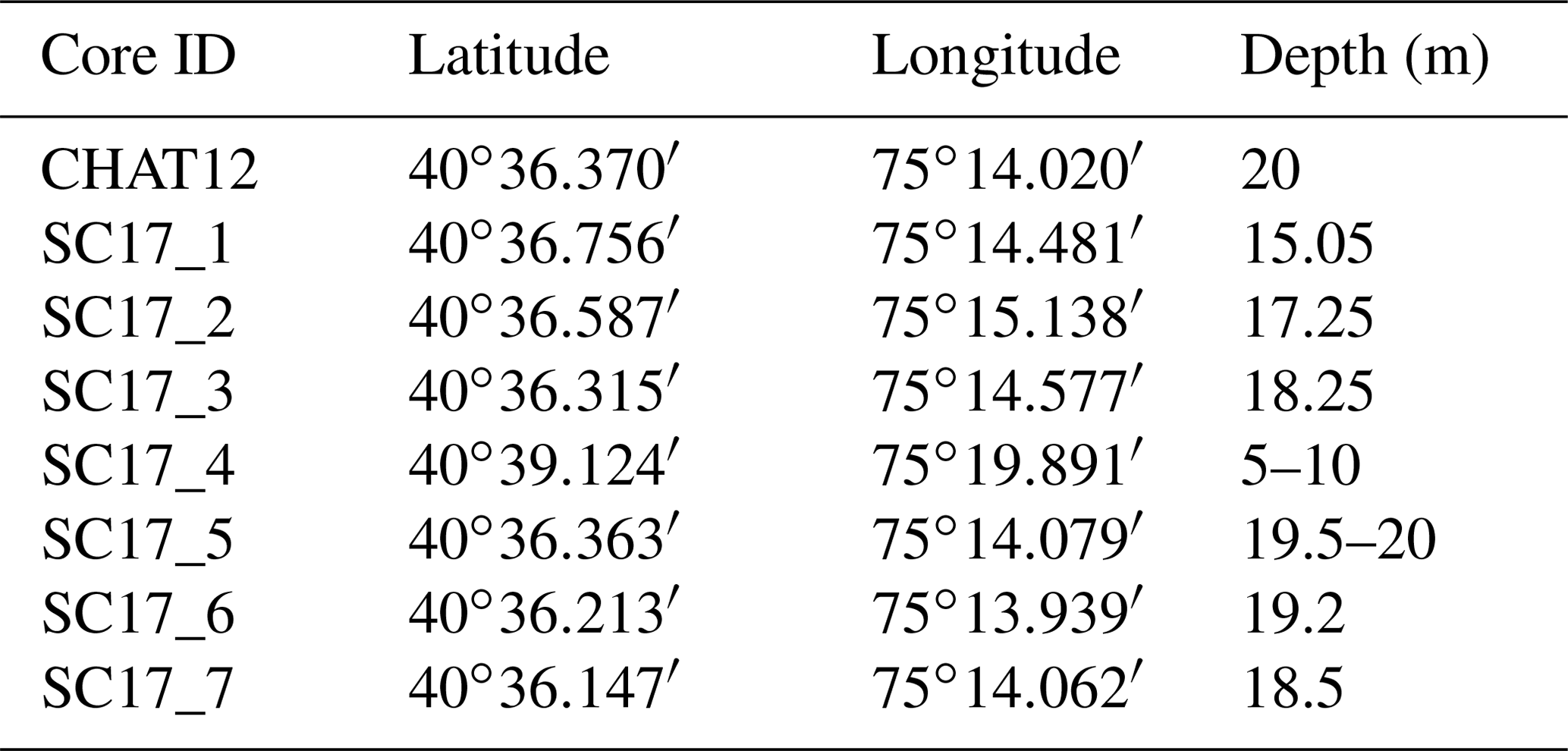
Five parallel cores each of 3 to 6 m length have been retrieved in 2012 from the deepest part of the lake ($\mathrm{40}{}^{\circ }{\mathrm{36.37}}^{\prime }$ N, $\mathrm{75}{}^{\circ }{\mathrm{14.02}}^{\prime }$ E) by using an UWITEC piston corer (Fig. 1, Table 1). All cores were opened, split, and photographed at GFZ Potsdam, where they are archived in a cold store at 4 ^∘C. A continuous composite profile of 623.5 cm length (CHAT12) was established by correlating the individual, overlapping cores via macroscopically visible marker layers (Fig. 3). Furthermore, seven parallel gravity cores (SC17_1-7) have been retrieved with a UWITEC gravity corer in 2017 (Fig. 1, Table 1) to recover the undisturbed sediment–water interface, from which the best-preserved parallel core, SC17_7, was used for gamma spectrometric analysis.

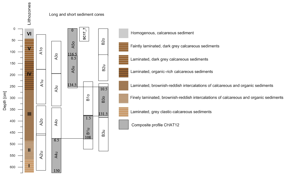
Figure 3 The composite profile CHAT12 (dark grey: piston cores A5o, A5u, B3o, B1u, and A4u; depth sections that were used are displayed within). Additional gravity cores taken in 2017 (SC17_1 to SC17_7) were only partly used for thin section preparation and gamma spectrometry dating. The gravity cores cover approximately the upper first metre of the composite profile.

Table 1 Coordinates of long and short cores.

3.2 Sediment micro-facies analysis and varve counting

Continuous 10 cm long sediment slabs with an overlap of 2 cm were taken from the whole composite profile to prepare large-scale petrographic thin sections. Thin section preparation followed the method described by Brauer and Casanova (2001) and included freeze-drying and vacuum impregnation of the sediment slabs with Araldite epoxy resin. Microfacies analysis, including a semiquantitative evaluation of planktic and periphytic diatoms, aquatic plant remains (e.g. Potamogeton sp., Ruppia maritima), ostracods, daphnia, characeae and chrysophytes, was carried out on a Zeiss Axioplan microscope using different magnifications (25–400×) and included measurement of varve thicknesses, micro-facies/varve type characterization, the definition of varve boundaries, and the development of process-related deposition models. A varve quality index (VQI) ranging from 0 to 5 was given for each varve, which is comparable to the method from Żarczyński et al. (2018) and references therein.

• VQI 0 represents no varves or strongly disturbed varved sequences and no reliable counting (interpolation).

• VQI 1 represents very low varve preservation, horizontally discontinuous varve, less well-preserved sublayer boundaries, and difficult counting.

• VQI 2 represents low varve preservation, occasional horizontally discontinuous varve and sublayer boundaries, and reliable counting.

• VQI 3 represents medium varve preservation, horizontally continuous varve and sublayer boundaries, only small disturbances, and reliable counting.

• VQI 4 represents high varve preservation, clearly distinguishable varve and sublayer boundaries, and reliable counting.

• VQI 5 represents highest varve preservation, clearly distinguishable varve and sublayer boundaries, no disturbances, and reliable counting.

Varve counting was performed to establish a floating varve chronology. Non-varved intervals (VQI =0) between varved sediment sections were therefore interpolated by using the mean of sedimentation rates derived from about 20 varves above and below the non-varved part. Varves were counted twice by the same author. Counting uncertainty estimates were first assessed by the percentage deviation of the second to the first count within one thin section. The mean of these deviations was used as an overall counting uncertainty estimate and assigned to the entire varved record. The uncertainty estimates were thus also assigned to interpolated sequences.

3.3 XRF element mapping

X-ray fluorescence (XRF) element mapping was performed on two selected Araldite impregnated sediment blocks (ca. 2 cm×10 cm), which were prepared for thin sections used for the micro-facies analyses. XRF element mapping of these two sediment blocks allows for linking micro-facies analyses of typical varve types directly with geochemical sediment compositions. Element mapping was performed at 50 µm resolution and covering most of the surface of the sediment block (15 mm×100 mm) using a Bruker M4 Tornado at GFZ Potsdam. This scanner is equipped with a Rh X-ray source operated at 50 kV and 600 µA in combination with poly-capillary X-ray optics that irradiate a spot of 20 µm for 50 ms. After measuring and an initial spectrum deconvolution, normalized element intensities are used to visualize relative element abundances as 2D maps.

3.4 Radiometric dating

3.4.1 Radiocarbon dating

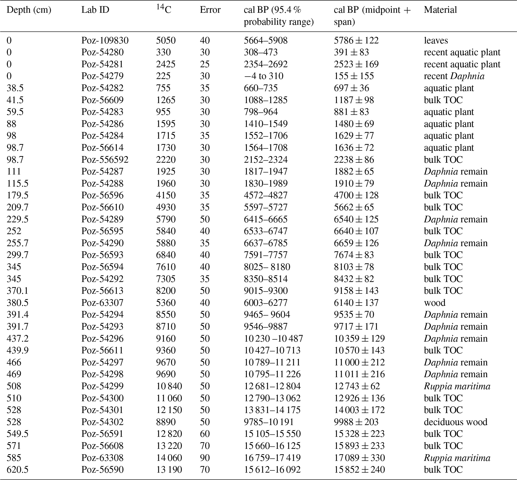
In total, 36 accelerator mass spectrometry (AMS) ¹⁴C measurements were carried out at the Pozńan Radiocarbon Laboratory in Poland. Samples for ¹⁴C measurements comprised two pieces of wood, bulk TOC (total organic carbon) samples, aquatic plant macro remains, daphnia remains, and Ruppia maritima seeds (Table 2). Additional samples of recent living daphnia and aquatic plants have been collected to assess the modern ¹⁴C reservoir effect. The resulting conventional ¹⁴C ages were calibrated using OxCal 4.3 (Ramsey, 2009) with the IntCal13 calibration curve (Reimer et al., 2013).

Table 2 ¹⁴C dates (calibrated with OxCal 4.3, IntCal13).

3.4.2 Gamma spectrometry dating

Gamma spectrometry measurements were performed on 0.5 cm thick sediment slices that were continuously sampled from the upper 15.0 cm of gravity core SC17_7 (Supplement Table S1). The samples were freeze-dried and sieved through a 200 µm mesh for homogenization and removal of larger plant particles. Individual sample-aliquots were filled into gas-tight sealable low-activity Kryal© tubes at identical fill heights and accurately weighted. After sufficient in-growth time, the gamma energies of ²¹⁰Pb ($T_{\mathrm{1}/\mathrm{2}}=\mathrm{22}$ yr) and ²¹⁴Pb ($T_{\mathrm{1}/\mathrm{2}}=\mathrm{26.8}$ min), which is a daughter nuclide of ²²²Rn ($T_{\mathrm{1}/\mathrm{2}}=\mathrm{3.8}$ d), were measured at 46.54, 295.24, and 351.93 keV. In addition, the gamma energies of ¹³⁷Cs ($T_{\mathrm{1}/\mathrm{2}}=\mathrm{30.1}$ yr) were measured at 661.66 keV. For this purpose, the Kryal© tubes were placed into shielded measurement chambers equipped with two well-type germanium detectors, G1 and G2 (Canberra Industries), for ∼1.5 to 7 d at GFZ Potsdam (Supplement Table S1) (Schettler et al., 2006). Hardware control, data storage, and spectrum analysis were realized with the software Genie 2000 (Canberra Industries). The average counting uncertainty was 5.9 % for ²¹⁰Pb, 7.7 % (295 keV) and 3.7 % (351 keV) for ²¹⁴Pb, and 5.2 % for ¹³⁷Cs. Efficiency calibrations were carried out for ²¹⁰Pb, ²¹⁴Pb, and ¹³⁷Cs with the same analytical setup using an internal laboratory standard and the “Loess Nussloch” standard (Potts et al., 2003). Blank activities for ¹³⁷Cs were negligible, while average ²¹⁰Pb blank activities of 10 mBq g⁻¹ for detector G2 and ²¹⁴Pb blank activities of 9 mBq g⁻¹ for the detectors G1 and G2 were considered. The activity measurements of ²¹⁴Pb were used to quantify the proportion of supported ²¹⁰Pb (²¹⁰Pb_supp) produced by the decay of ²²⁶Ra in the sediment. The activity of unsupported ²¹⁰Pb (²¹⁰Pb_unsupp) in the sediment, which originates from the decay of ²²²Rn in the atmosphere and associated aeolian deposition, is quantified by the difference between measured ²¹⁰Pb_total and ²¹⁰Pb_supp. We selected sections that showed linear correlations in the semi-logarithmic plot of ²¹⁰Pb_unsupp versus depth to infer average sedimentation rates using the constant initial concentration (CIC) model (cf. Appleby, 2002) (Supplement Table S2). Intercalated sediment sections showed nearly uncorrelated ln(²¹⁰Pb_unsupp) vs. depth relationships at 10.25–9.25, 6.25–4.25, and 2.25–1.75 cm depths (Supplement Fig. S3). Therefore, the initial ²¹⁰Pb_unsupp activities of samples that bridged these sections were used alternatively to determine time intervals between these samples to infer a chronology. To assess possible changes of the sedimentation regime, we additionally calculated sedimentation rates of each 0.5 cm thick sediment slice using the CRS model (constant initial ²¹⁰Pb_unsupp supply) (cf. Appleby, 2002; Appleby and Oldfield, 1978) (Supplement Table S3).

4 Results

4.1 Lithology

The composite profile can be subdivided into six lithological units (Fig. 3). Lithozone I (LZ I) from 623.5 to 566.0 cm depth consists of greyish-brownish clastic-calcareous sediments. It shows millimetre-scale laminations of fine sandy and silty-to-clayey layers. LZ II (566.0–480.0 cm) exhibits intercalations between horizons of very fine millimetre-scale laminated brownish-reddish organic-rich sediments and sections with greyish calcareous sediments. Brownish-reddish intercalating horizons of millimetre-scale laminated organic and calcareous sediments characterize LZ III from 480.0 to 273.0 cm depth. LZ IV (273.0–130.0 cm) is characterized by brownish-reddish millimetre-scale laminated organic-rich sediments with intercalated horizons rich in aquatic plant remains, which occur at 232.0–223.0, 185.0–180.0, and 164.0–130.0 cm depths. LZ V (130.0–41.0 cm depth) starts with a 16 cm thick interval of dark grey millimetre-scale laminated calcareous sediments, followed by brown millimetre-to-centimetre-scale laminated sediments until 41.0 cm depth. Laminations are only poorly preserved between 63.0 and 41.0 cm depth. The uppermost sediments of LZ VI (41.0–0.0 cm depth) consist of homogenous brownish-greyish calcareous sediments, which are rich in aquatic plant remains. The uppermost centimetre is enriched in calcite and exhibits greyish faint laminations.

4.2 Sediment micro-facies analysis

Microscopic sediment analysis revealed that clastic sublayers are present throughout the finely laminated sediments below 63.0 cm depth (Fig. 4a). These clastic sublayers are variably intercalated with calcitic, aragonitic, and organic sublayers and thus form different types of cyclic successions. In total, we classified six different types of sublayer successions as described below. The name for these types reflects the dominant sublayer for each of the six types. For example, the clastic-organic type is characterized by the dominance of clastic sublayers, while in the organic-clastic type organic sublayers dominate. The names are not related to the order of sublayer succession within each type. The changing dominance of different sublayer successions reflects the lithozones.

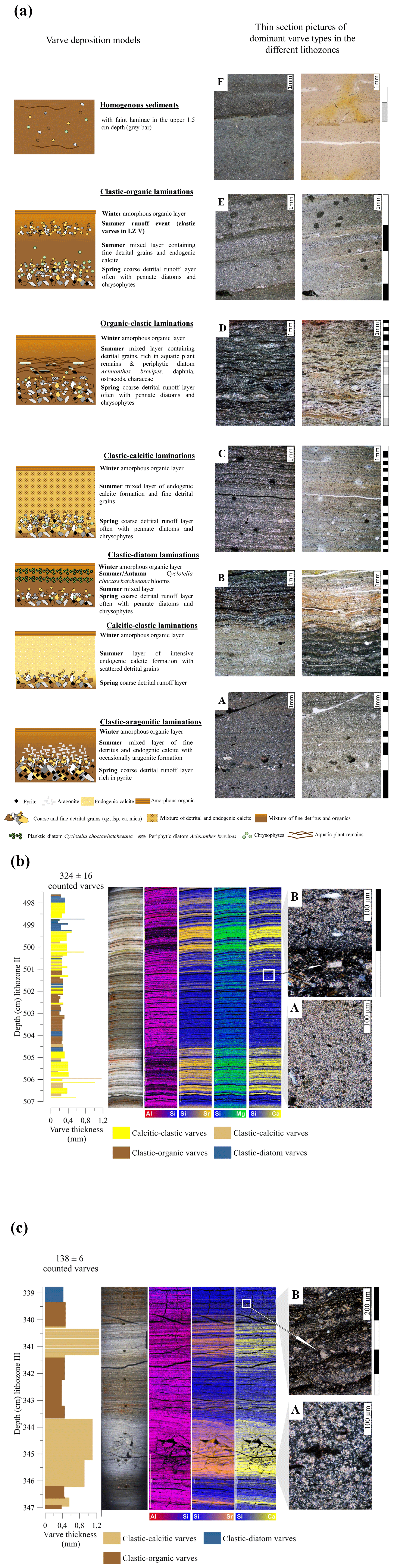
Figure 4 (a) Thin section pictures of different lamination (varve) types in cross-polarized (left) and plane polarized (right) light of the different lithozones LZ I to LZ V. (A) Clastic-organic laminations; (B) intercalation of clastic-organic, clastic-diatom and calcitic-clastic laminations; (C) intercalation of clastic-calcitic, clastic-organic, and clastic-diatom laminations (upper part); (D) organic-clastic laminations; (E) clastic-organic laminations; (F) homogenous sediments. Black/white/grey bars alongside the thin section pictures indicate one individual varve, but the reliability of grey bars (varves) is generally lower due to large amounts of aquatic plant remains and low preservation. Process-related deposition models of the observed lamination/varve types illustrate the seasonal depositional successions (A–E). (b) XRF map 1: varve types and XRF element mapping of a thin section from LZ II from 507 to 497.5 cm depth. Element maps show an alternation of siliciclastic sediments with large amounts of Si and Al with calcite layers (Ca) with large amounts of Sr and Mg according to the presence of clastic-organic, clastic-diatom, clastic-calcitic, and calcitic-clastic varves, respectively. Micro-facies analyses show endogenic calcite within calcitic-clastic varves within the summer sublayer (image A). Clastic-organic and clastic-diatom varves are indicated by large amounts of Si and Al with only individual calcite (arrow image B) and Mg-calcite grains. Note that coinciding occurrences of individual elements result in colour mixing; for example, Al (red) and Si (blue) become pink. Endmembers of the Al–Si map are indicative for the presence of Al-rich clays and diatomaceous Si. (c) XRF map 2: varve types and XRF element mapping of a thin section from LZ III from 357 to 338.5 cm depth. Element maps show an alternation of siliciclastic sediments with large amounts of Si and Al with calcitic layers (Ca) with large amounts of Sr according to the presence of clastic-organic, clastic-diatom, and clastic-calcitic varves, respectively. Micro-facies analyses show mixed calcitic (resuspended and endogenic) summer sublayers within clastic-calcitic varves (image A). Clastic-organic and clastic-diatom varves are indicated by large amounts of Si and Al with only individual calcite grains (arrow, image B). Note that coinciding occurrences of individual elements result in colour mixing; for example, Al (red) and Si (blue) become pink. Endmembers of the Al–Si map are indicative for the presence of Al-rich clays and diatomaceous Si (blue).

4.2.1 Clastic-aragonitic type

Clastic-aragonitic laminae are rare (2.7 %), mainly occurring in LZ I and particularly at 600.0–605.0 and 609.0–616.0 cm composite depths. This subtype is composed of three sublayers, and the mean thickness is 0.59 mm (Figs. 4a (A), S2a). These laminae exhibit the general pattern of clastic-organic laminae in LZ I, with a coarse-grained and thick basal detrital sublayer, but the overlying mixed (detrital calcite, mica, fsp (feldspar), qtz (quartz), and medium amounts of endogenic calcite) fine-grained sublayer additionally contains idiomorphic aragonite needles that are not found in clastic-organic varves. The sublayer succession ends with an amorphous organic matter sublayer.

4.2.2 Calcitic-clastic type

The deposition of calcitic-clastic laminae (6 %) with a dominating endogenic calcite sublayer is restricted to LZ II. This subtype is composed of three sublayers and the mean thickness is 0.41 mm, with a maximum of 2.0 mm. Calcitic-clastic laminae (Figs. 4a (B) lower part, S2b) are usually characterized by a basal detrital sublayer, which, however, is not developed in all calcitic-clastic laminae. The overlying sublayer generally exhibits low species abundances of diatom frustules, chrysophyte cysts, aquatic plant remains, daphnia, ostracods, and characeae but massive and fine-grained endogenic calcite, which is not the case in the clastic-calcitic laminae subtype. Endogenic calcite formed in the water column (Fig. 4b (A)) is recognized by its well-developed idiomorphic rhombohedral shapes. Scattered detrital grains occasionally occur within the endogenic calcite matrix. One depositional cycle ends with an amorphous organic matter sublayer.

4.2.3 Clastic-diatom type

Clastic-diatom laminae (20 %) occur in LZ II, LZ III, and LZ IV. This subtype is composed of three sublayers and the mean thicknesses vary from 0.28 mm (LZ II) via 0.34 mm (LZ III) to 0.35 mm (LZ IV). The depositional cycle starts with a basal detrital sublayer, which is overlain by a finer-grained mixed sublayer (detrital calcite, mica, fsp, qtz) occasionally containing chrysophytes and different diatom taxa. The third sublayer is formed by diatom blooms exclusively consisting of the planktic diatom species Cyclotella choctawhatcheeana (Anja Schwarz, TU Braunschweig, personal communication, 2019) (Figs. 4a (B) upper part, S2c).

4.2.4 Clastic-calcitic type

The second most common lamina subtype (23.5 %) is clastic-calcitic laminae (Figs. 4a (C) lower part, S2d), which are most abundant in LZ I, LZ II, LZ III, and LZ V. This subtype is composed of four to five sublayers, and the mean total thicknesses are 0.95 mm (LZ I), 0.35 mm (LZ II), 0.72 mm (LZ III), 1.56 mm (LZ IV), and the maximum value of 5.0 mm in LZ V. Clastic-calcitic laminae exhibit a basal detrital sublayer with a sharp lower boundary, which is followed by a bloom layer of chrysophytes and/or diatoms, occurring sporadically after and/or within the detrital sublayer. The third overlying mixed sublayer contains medium amounts of endogenic as well as fine-grained detrital calcite (Fig. 4c (A)), as well as mica, fsp, and qtz grains, but low amounts of diatom frustules and chrysophyte cysts. One depositional cycle typically ends with an amorphous organic matter sublayer. In LZ V, these clastic-calcitic laminae occasionally contain a very fine-grained, light greyish, micritic sublayer before the cycle ends with the amorphous organic sublayer.

4.2.5 Organic-clastic type

Horizons of organic-clastic laminae (5.2 %) with dominating organic sublayers are mainly present within LZ IV and LZ V (Figs. 4a (D), 2e), particularly at 261.0–252.0, 176.0–173.0, 150.0–126.0, and 122.0–110.0 cm depths. This subtype is composed of three sublayers and the mean thicknesses being 0.49 mm (LZ IV) and 1.64 mm (LZ V) with a maximum of 9 mm in LZ V. Organic-clastic laminae exhibit an often horizontally discontinuous basal detrital sublayer (lens-shaped) in LZ IV, which is overlain by a mixed sublayer that contains detrital calcite, mica, fsp, and qtz grains, and many aquatic plant remains and periphytic diatoms (Achnanthes brevipes, Anja Schwarz, TU Braunschweig, personal communication, 2019), whose colony chains are often preserved. One deposition cycle ends with a yellowish amorphous organic matter layer.

4.2.6 Clastic-organic type

Clastic-organic laminae are present in all lithozones and most abundant in the record (42.5 % of all observed and measured laminae). This micro-facies type is composed of four sublayers of which the most prominent is a basal clastic-detrital sublayer with a sharp lower boundary. The basal detrital sublayer contains mainly detrital calcite which is distinguished from endogenic calcite by microscopic analyses. Detrital calcite is characterized by irregularly shaped grains and generally larger grain sizes of average of 0.6 mm and up to 1.82 mm in LZ I. Detrital layers further contain siliciclastic minerals such as mica, quartz (qtz) and feldspars (fsp). This basal layer is often, but not regularly, overlain by chrysophyte and/or diatom blooms and a third mixed sublayer containing mainly fine-grained detrital calcite, mica, fsp, and qtz with small amounts of endogenic calcite and varying amounts of diatom frustules, chrysophytes, characeae, ostracods, and daphnia. The deposition cycle ends with a yellowish layer of amorphous organic material.

The mean thickness of clastic-organic laminae differs between the lithozones. In LZ I, the mean thickness is 0.59 mm with a maximum thickness of 3.1 mm. In LZ I, the basal detrital sublayer is thick and coarse grained; rich in pyrite; and contains mainly silty-to-fine sand-sized grains and occasionally sand-sized qtz, calcite, and fsp grains, whereas diatoms and chrysophytes are rare. In LZ II and LZ III, clastic-organic laminae are less thick with mean thicknesses of 0.27 and 0.48 mm, respectively. In these lithozones, the basal sublayer contains no sand-sized particles. In LZ IV, mean varve thickness is 0.43 mm and the basal sublayer is often lens-shaped and horizontally discontinuous. In LZ V, between 130.0 and 63.0 cm depth, thickest clastic-organic laminae occur with a mean thickness of 1.5 mm and a maximum thickness of up to 7.0 mm (Figs. 4a (E), S2f). These clastic-organic laminae often include an additional detrital sublayer intercalated in the finer-grained mixed sublayer.

4.2.7 Homogenous sediments

The uppermost 41.0 cm of the sediment record consists of homogenous sediments, containing a fine-grained mix of autochthonous and allochthonous calcite, mica, qtz, and fsp. The sediments are generally rich in organic remains, such as aquatic plant remains, chrysophytes, diatoms, and chlorophytes (Botryococcus). Faint and discontinuous calcite laminae occur in the uppermost centimetre (Fig. 4a (F)).

4.3 XRF element mapping

The two selected impregnated sediment blocks from 507 to 497.5 cm (XRF map 1 Fig. 4b) and from 346.5 to 338.5 cm depths (XRF map 2 Fig. 4c) contain calcitic-clastic, clastic-diatom, clastic-calcitic, and clastic-organic micro-facies types. These sediments are dominated by alternating calcitic and siliciclastic sediments represented by the elements Ca, Sr, Mg, Si, and Al, respectively (Fig. 4b and c). Colour variations of the element maps show that the calcitic and siliciclastic sediments are clearly separated in the XRF map 1 sample (Fig. 4b) but slightly more mixed in the XRF map 2 (Fig. 4c). In both XRF maps 1 and 2, the carbonate sublayers are enriched in Sr (Fig. 4b and c), whereas in the XRF map 1 the additional enrichment of Mg (Fig. 4b) indicates the presence of Sr- and Mg-rich carbonates. Microfacies analysis shows that Mg- and Sr-rich calcite sublayers in XRF map 1 are predominantly of endogenic origin (Fig. 4b (A)), whereas the Sr-rich calcite layers in XRF map 2 contain mixed endogenic and resuspended calcites (Fig. 4c (A)). Moreover, detrital carbonates occur predominantly as individual grains in the siliciclastic sediments and sublayers and are shown by Ca and Mg in the XRF element maps (Fig. 4b (B) and 4c (B)). Siliciclastic muds of clastic-organic and clastic-diatom varves are represented by the co-occurrence of Al and Si in the XRF element maps, whereas Al is absent in diatomaceous sublayers (Fig. 4b and c).

4.4 Chronology

4.4.1 Floating varve chronology (623.5–63.0 cm)

A floating varve chronology labelled as Chatvd19 (Fig. 5b) was established for the composite profile below 63.0 cm depth and comprises a total of 11 259 counted and interpolated varves. Based on the interpretation of laminations as varves, 9026 of the total 11 259 varves were counted, which is equal to 80.2 %. The first varve count reveals 9026 varves and is the base for the floating varve chronology. Although the total varve number of 8955 obtained by the second count is very similar to the first count, larger deviations between the two varve counts in individual sediment sections occur throughout the sediment record due to varying stages of varve preservation as expressed in the VQI (Fig. 5a). The largest deviations occur in LZ I (603.0–595.0 cm) with 23.7 %, in LZ II (490.0–484.0 cm) with ∼13 %, in LZ III (413.0–405.0 cm) with ∼16 %, in LZ IV (141.0–134.0 cm depth) with 19.5 %, and in LZ V (65.0–63.0 cm depth) with 7.7 %. The lowest deviations (<1 %) were obtained in LZ II at 539.0–530.0 and 498.0–490.0 cm; in LZ III at 451.0–445.0, 421.0-413.0, 375.0–369.0, 299.0–290.0, and 282.0–275.0 cm; in LZ IV at 197.0–190.0 cm; and in LZ V at 125.0-119.0, 116.0–113.0, and 73.0–65.0 cm depth. Interpolated sequences are unevenly distributed within the record and are mainly present within LZ IV. The longest interpolated sequences occur in LZ IV with ∼5 cm from 198.0–193.0 cm depth and in LZ III with almost 7 cm between 444.0 and 437.0 cm depth. A VQI (Fig. 5a) of 1 is represented by 5.6 % of the total varves, VQI of 2 by 8.4 %, VQI of 3 by 26.4 %, VQI of 4 by 18.3 %, and VQI of 5 by 21.4 %. The calculated mean deviation between the two varve counts of ∼5 % (Fig. 5a) is used as a conservative uncertainty for the floating varve chronology to consider high uncertainties in individual sediment sections in a more realistic way, despite the similar total number of varves counted. The floating varve chronology has a basal age of 11 619±603 BP.

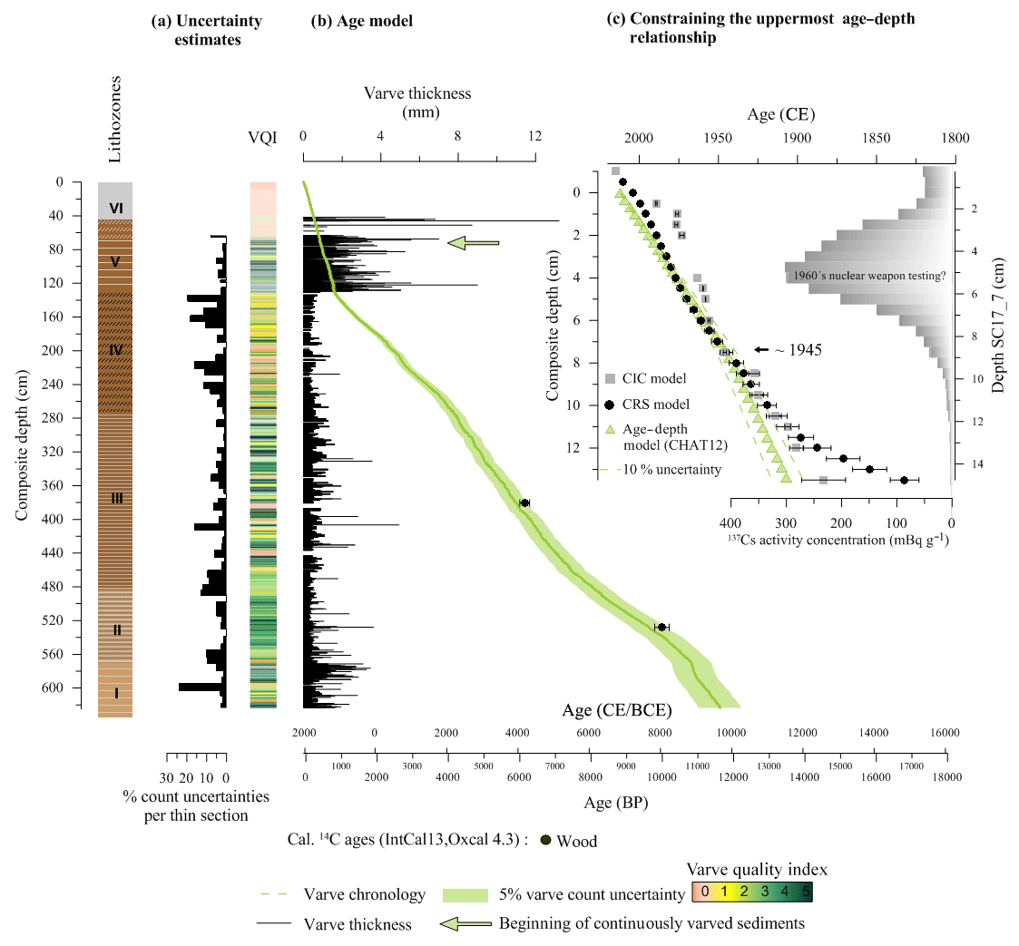
Figure 5 (a) Varve counting uncertainty estimates (mean of 5 % is green) and VQI distribution. (b) Age model of the floating varve chronology (Chatvd19) from 63.0 to 623.5 cm depth with a basal age of 11 619±603 BP (light green). The black line shows the measured varve thickness and black dots mark the distribution of calibrated AMS ¹⁴C ages (with 95.4 % probability range) of wood pieces (Table 2). (b) ²¹⁰Pb CIC (grey squares) and CRS (black dots) age models; ¹³⁷Cs activity concentration profile and constrained age model for the uppermost part of the composite profile (green triangles).

4.4.2 Chronology of the non-varved uppermost sediments

The uppermost 63.0 cm of the sediment profile are not varved and thus require alternative dating approaches including ²¹⁰Pb dating, activity profiles of ¹³⁷Cs, and sedimentation-rate-based interpolation. First, we measured ²¹⁰Pb activity concentrations of the uppermost 15 cm of short core SC17_7 and applied the CIC and CRS models (Figs. 5c and 6, Supplement Table S3). SC17_7 is correlated to the composite profile through macroscopically visible facies change at 1.0 cm composite depth and through a laminated section from 45.0 to 41.0 cm composite depth (Supplement Fig. S1). The CIC and CRS model-based chronologies are broadly consistent and particularly date sediments at 8.75 cm (SC17_7) or 7.5 cm composite depth to 1945/1946 CE (Figs. 5c and 6b, Supplement Table S3). This coincides with the onset of increased ¹³⁷Cs activity concentrations (Figs. 5c, 6c), marking the onset of nuclear weapon testing in 1945 CE (Bergkvist and Ferm, 2000; Kudo et al., 1998; Norris and Arkin, 1998). Therefore, we applied the date of 1945 CE (8.75 cm in core SC17_7) as an anchor point for the chronology of the uppermost 63.0 cm of the composite profile. According to micro-facies-based sedimentological correlation, this anchor point is located at 7.5 cm composite depth. The section of homogeneous sediments from this point down to 63.0 cm depth was interpolated. This interpolation is based on sedimentation rate calculations obtained by lead-210 dating and varve thickness measurements in adjacent sediment intervals. Calculations include sedimentation rates from the upper 7.5 cm (1.12 mm yr⁻¹), from 15 varves (1.9 mm yr⁻¹) between 41.0 and 63.0 cm depth, and from 100 varves (1.66 mm yr⁻¹) below 63.0 cm depth, and they result in a mean SR of 1.56 mm yr⁻¹, corresponding to 356 interpolated years. Adding the number of 356 interpolated years to the radiometric date of 1945 CE results in an age of 1589 CE (360 BP) at 63.0 cm depth. We assume a conservative uncertainty of ca. 10 % as a maximum error for our interpolation. The anchor point thus has an age of 360±40 BP. The uncertainty of this anchor point is added to the varve counting uncertainty.

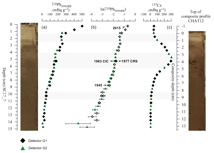
Figure 6 Gamma spectrometry results of the gravity core SC17_7. Light grey intervals indicate uncorrelated sequences of the ln²¹⁰Pb_unsupp vs. depth profile which affected the CIC model calculations (Supplement Fig. S2, Supplement Tables S2, S3). Core pictures of the upper part of the composite profile CHAT12 (right) and the gravity core SC17_7 (left) illustrate the facies change to calcite-enriched sediments in the uppermost centimetre.

4.4.3 Radiocarbon dating

In total, we dated 36 samples of bulk organic carbon, daphnia remains, aquatic plant remains, and Ruppia martima seeds. Only two samples were terrestrial plant remains (wood fragments) and sufficiently large to be used for AMS ¹⁴C dating (Table 2, Figs. 5 and 7). Except the two ages from terrestrial plant remains (Poz-54302 with 9988±203 cal BP and Poz-63307 with 6140±137 cal BP), all other ages deviate from the varve chronology between 155 years at 0.0 cm depth and 6150 years at 585.0 cm depth (Fig. 7). We observe a general trend of decreasing deviations up core with the maximum deviation of ∼6150 years at 585.0 cm depth in LZ I. Looking at more detail, the deviations between radiocarbon and varve ages exhibit a prominent stepwise increase particularly at the boundary between LZ IV and LZ V when it abruptly decreases from ∼3000 to ∼1000 years. Modern aquatic plants collected during the field campaign in 2012 showed large modern reservoir ages of 330±30 and 2425±25 ¹⁴C years, and living daphnia yielded ages of 225±30 ¹⁴C years.

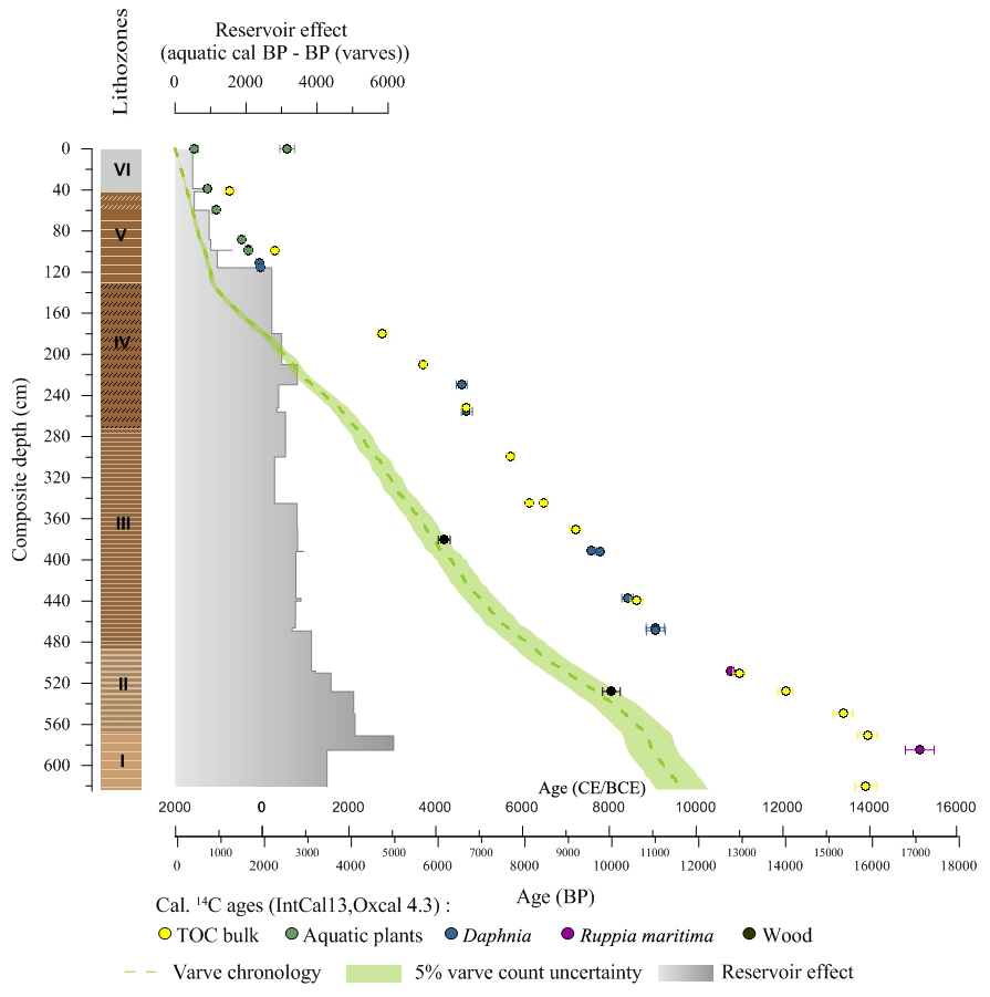
Figure 7 Radiocarbon reservoir effect (grey step plot). The reservoir effect was determined by the difference between aquatic (cal BP) (coloured symbols) and varve ages (green). Floating varve chronology (green) and distribution of calibrated AMS ¹⁴C ages (with 95.4 % probability range) of wood pieces, TOC bulk, aquatic plant remains, daphnia, and Ruppia maritima remains (Table 2).

5 Discussion

5.1 Interpretation of fine laminations as varves

The construction of varve chronologies relies on the proof of seasonal origin of fine laminations (Brauer et al., 2014; Ojala et al., 2012; Zolitschka et al., 2015). Laminations are absent in the upper 63.0 cm of the Chatyr Kol lake sediment core and cyclic successions of mixed clastic laminations are only observed below this depth. Therefore, the seasonal origin of the Chatyr Kol sediments cannot be proved through modern observation in sediment traps, because no varves are formed in the present day. Instead, we applied process-related deposition models (Fig. 4a) based on detailed micro-facies analyses obtained from petrographic thin sections and compared our observations with varve types described in literature (Brauer, 2004; Zolitschka et al., 2015). We associate the observed successions of different types of mixed clastic laminations with the formation of different seasonal sublayers that are known from lakes with carbonaceous catchments (Brauer and Casanova, 2001; Kelts and Hsü, 1978; Lauterbach et al., 2011, 2019) and high-altitude glacial environments (Guyard et al., 2007; Leemann and Niessen, 1994). The observed successions of sublayers are interpreted as mixed varve types (clastic, organic, and endogenic) as defined by Zolitschka et al. (2015).

Varve formation at Chatyr Kol lake is related to the high seasonality of the local climate with an ice cover during winter as well as strong annual variations of the temperature and precipitation affecting productivity, endogenic carbonate formation, and local runoff. Varve preservation is promoted by the unique morphology of the deep western lake basin, where anoxic bottom water conditions can be maintained even under relatively low lake levels (Fig. 2).

We interpret the annual sedimentary cycle to always start with the deposition of a basal detrital sublayer with a sharp lower boundary, which results from winter/spring snow and/or glacial melt (Guyard et al., 2007; Leemann and Niessen, 1994; Zolitschka et al., 2015) after the ice break-up around April (Shnitnikov et al., 1978). Runoff with suspended sediment load is then likely directed through the Kegagyr River in the east but may also be the result of surface runoff through the activation of several widely distributed smaller tributaries in the catchment (Fig. 1).

Basal detrital sublayers are generally overlain by blooms of chrysophytes and/or diatoms within clastic-organic, organic-clastic, clastic-diatom, and clastic-calcitic varve types. Chrysophytes and/or diatom blooms develop as a consequence of the available nutrients provided by runoff and spring overturn in combination with rising temperatures during the summer season (Zolitschka et al., 2015). The productive phase in calcitic-clastic varves is, however, reflected by calcite precipitation, which is the main carbonate phase (endogenic, detrital, and resuspended) in the Chatyr Kol sediments. The formation of endogenic calcite in Chatyr Kol lake is controlled by (1) photosynthesis, when high aquatic productivity lowers the concentrations of CO₂, increases the pH of the lake water, and leads to a reduced solubility of ${\mathrm{CO}}_{\mathrm{3}}^{\mathrm{2}-}$ (Hodell et al., 1998; Kelts and Hsü, 1978; Zolitschka et al., 2015); (2) evaporation leading to an oversaturation of carbonate ions; and (3) sufficient supply of dissolved cations either through surface runoff or groundwater inflow (Shapley et al., 2005). Changes in weathering and hydrological conditions can lead to variations in the supply of Ca²⁺ and Mg²⁺ ions and subsequently change the Mg∕Ca ratio of the lake water (Müller et al., 1972). The formation of aragonite requires high lake water Mg∕Ca ratios (>12), whereas magnesium-calcite forms at lower Mg∕Ca ratios (Kelts and Hsü, 1978; Müller et al., 1972). XRF element intensity maps do not provide quantitative results but do indicate that Mg is abundant in the XRF map 1 from LZ II, which results in the formation of endogenic Sr- and Mg-rich calcites (Fig. 4b (A)).

Aragonite precipitates, related to an evaporative concentration in summer, were only microscopically observed in the intervals between 600.0 and 605.0 cm and between 609.0 and 616.0 cm composite depth, suggesting that Mg∕Ca ratios probably remained above Mg∕Ca ratios >12.

After the spring-to-early-summer lake productivity, the deposition of a mixed sublayer consisting of silt- to clay-sized detrital grains and small-to-medium amounts of endogenic calcite is observed in all lamination types (Figs. 4a, S2). In clastic-calcitic varves, the mixed sublayers appear different and include especially resuspended calcite as evidenced also in Ca and Sr intensities (Figs. 4a (C), 4c (A), S2d). The mixed sublayer indicates resuspension of shore material (littoral calcite) to the core location due to, for example, wind-induced wave activity and weak runoff during the ice-cover-free season from around April to October (Shnitnikov et al., 1978).

The intercalation of discrete detrital layers within the mixed sublayer (Figs. 4a (E), S2e), as observed in clastic-organic laminae in LZ V, indicates pulses of runoff of suspended material which may be caused by late rainfall events in summer (Aizen et al., 2001; Shnitnikov et al., 1978).

One annual depositional cycle usually ends with the deposition of a thin sublayer of very fine amorphous organic matter which is deposited under quiet water conditions when the lake was ice covered (Fig. 4a). In lithozone V, an additional micritic sublayer is deposited before the amorphous organic sublayer at the end of the seasonal cycle in clastic-calcitic laminae when water turbulence is low.

5.2 Varve counting and chronology construction

The interpretation of different types of fine laminations allowed for varve counting as a main tool for constructing the Chatyr Kol chronology largely based on incremental methods. Around 80 % of the varves in the sediment record are double counted in petrographic thin sections, while the remaining part of ca 20 % had to be interpolated based on sedimentation-rate estimates due to poor varve preservation. The resulting chronology comprises 11 259 years and is anchored to the absolute timescale at 63.0 cm sediment depth supported by a combination of lead-210 dating and occasional sedimentation rate measurements as described below. The resulting age–depth model is within uncertainties in good agreement with two calibrated AMS ¹⁴C dates of wood pieces at 380.5 cm depth (6140±137 cal BP; Poz-63307) and at 528.0 cm depth (9988±203 cal BP; Poz-54302) (Fig. 5b, Table 2). The corresponding varve-based ages are 5905±320 and 9611±505 BP, respectively. As for all chronologies, uncertainties are inherent also to varve chronologies, which are commonly assessed via replicate counts (Brauer and Casanova, 2001; Lamoureux, 2001; Lotter and Lemcke, 1999; Ojala et al., 2012; Żarczyński et al., 2018; Zolitschka et al., 2015). However, there is no standard procedure on how to calculate and present the uncertainties (Ojala et al., 2012; Zolitschka et al., 2015). Commonly, mean values of replicate count differences, the difference of maximum and minimum counts, or their standard deviation is reported (Brauer et al., 2014; Ojala et al., 2012; Żarczyński et al., 2018; Zolitschka et al., 2015). Despite the inevitable increase of cumulative uncertainties with age or depth, systematic uncertainties arise and are caused by changes in varve preservation, strongly and abruptly varying sedimentation rates, and the challenging differentiation of varve types with complex structures (Ojala et al., 2012; Żarczyński et al., 2018; Zolitschka et al., 2015). The overall very small difference between the two counts of the Chatyr Kol varved record of only −71 varves is due to the compensating effect between over- and underestimations of varve counts throughout the record. For the floating varve chronology, we therefore compare the results for each individual thin section comprising between a maximum of 324 (506.8–497.6 cm) and a minimum of 13 (varves) (65.4–63.0 cm) (Figs. 5a, 8).

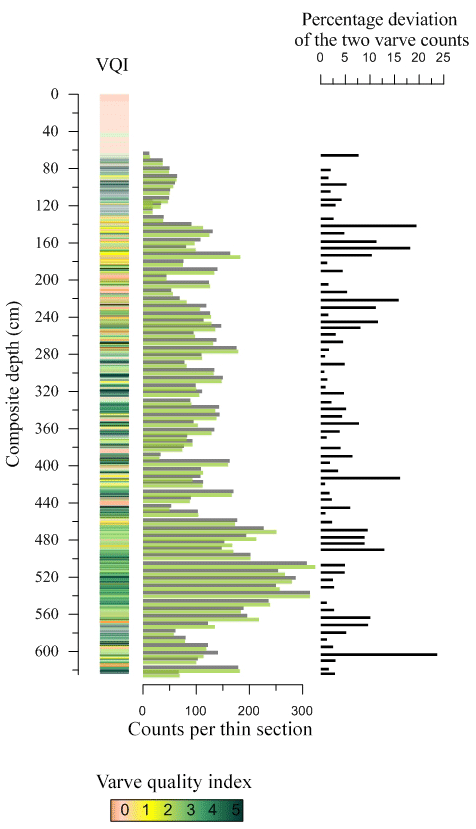
Figure 8 VQI counting differences for individual thin sections (green represents first count, black represents second count, and their percentage deviation is given).

Counting uncertainties for individual thin sections are reported as their percentage deviation from the first count used for the chronology and range between 0 % and 23.7 % (Figs. 5a, 8). Largest deviations of 23.7 % in LZ I are caused by a low visibility of varve boundaries and by coring artefacts. Deviations of ∼13 % in LZ II and of ∼16 % in LZ III result from the abrupt intercalations between clastic-organic, clastic-diatom, clastic-calcitic, and calcitic-clastic varve types with varying varve thicknesses (Fig. 4b, c). Deviations in LZ IV with a maximum of 19.5 % coincide with generally lowest VQI values (Fig. 8) and result from the domination of clastic-organic and organic-clastic varves with lowest thicknesses and discontinuous basal detrital sublayers (Fig. 4a (D)), leading to generally higher counting uncertainties. Lowest deviations of <1 % in LZ II, LZ III, LZ IV, and in LZ V represent best preservation and thus easily countable varves of different varve types. Generally, clastic-organic and clastic-calcitic varves with higher varve thickness, especially in LZ V, are most reliably countable. The relatively high uncertainties of 7.7 % in LZ V are due to the low number of varves comprised in individual thin sections (Fig. 8). For the total uncertainty estimate for the floating varve chronology, we use the mean of ±5 % calculated from the uncertainties for each 10 cm interval. This conservative estimate is more realistic than the very low difference in the two repeated varve counts. An uncertainty of 5 % is in the range of varve chronologies reported elsewhere (Ojala et al., 2012).

Since the uppermost 63.0 cm of the sediment profile is largely homogeneous, the varve chronology is floating and needs to be anchored to an absolute chronology at this point. The interpolation with a mean SR derived from the combination of the consistent CIC and CRS ²¹⁰Pb marker (1945 CE), the SR derived from discontinuously varved sequences between 41.0 and 63.0 cm depth, and from 100 measured varves below 63.0 cm depth seems to be the best approach for constraining the uppermost age–depth relationship within the homogenous sediments, where further chronological markers are lacking. We are aware that the interpolation-based “floating” anchor point at 63.0 cm depth is prone to additional uncertainties. We considered this by assuming a higher uncertainty of 10 % for this interval than that of ±5 % for the floating varve chronology.

5.3 Radiocarbon reservoir effects

Compared to the floating varve chronology, including two terrestrial (wood) AMS ¹⁴C dates, we observed a general trend of decreasing reservoir effects of dated aquatic material up core with the maximum deviation of ∼6150 years at 585.0 cm depth (10 930±570 BP) in LZ I (Fig. 7). The stepwise decrease of deviations between radiocarbon and varve ages is most pronounced at the boundary between LZ IV and LZ V, when it abruptly decreases from ∼3000 to ∼1000 years. The reservoir effect generally depends on the rate of atmospheric CO₂ exchange between the water column and the air, internal mixing dynamics, and the input of ¹⁴C-depleted carbonaceous material (Ascough et al., 2010; Jull et al., 2013; Keaveney and Reimer, 2012; Lockot et al., 2016; MacDonald et al., 1991). The catchment of Chatyr Kol lake exhibits several sources that could be responsible for a ¹⁴C depletion of dissolved carbon species in the lake water. Highest reservoir ages in the early Holocene are likely the result of the combined influence of these sources: (1) the input of old, ¹⁴C-depleted CO₂ with glacial meltwater (cf. Hall and Henderson, 2001) at the onset of a warming Holocene and (2) the weathering and erosion of the northern outcropping limestones, which led to the release and input of dissolved bicarbonate to the lake (cf. Abbott and Stafford, 1996; Hutchinson et al., 2004). Both processes lead to a ¹⁴C-depleted CO₂ and ${\mathrm{HCO}}_{\mathrm{3}}^{-}$ uptake during photosynthesis by, for example, submerged aquatic plants like Ruppia martima at 585.0 cm depth (Fig. 7) and by phytoplankton, on which daphnia feed and which therefore also show similar reservoir effects. A high detrital input and thus a potentially high input of dissolved bicarbonate is supported by increased varve thicknesses during the early Holocene (Sect. 5.4.1, Fig. 9). Furthermore, (3) thawing of permafrost since the beginning of a warming Holocene might have released dissolved ¹⁴C-depleted organic material and thus affect the ¹⁴C TOC bulk measurements. Our field-trip observations and observations by Shnitnikov et al. (1978) of modern permafrost reduction and the development of thermokarst in the southern part of the catchment around the neighbouring Maloye lake (Fig. 1) support this assumption. The cause of a stepwise reservoir effect reduction is therefore likely also related to the combined effect of a generally decreasing glacial influence and a decreasing input of bicarbonate until ∼ 1150 CE at the boundary between LZ IV and LZ V (Figs. 7, 9). The abrupt decrease of the reservoir effect after ∼ 1150 CE, despite an increase in detrital carbonate supply (Sect. 5.4.5, Fig. 9), might be related to the silting up of the basin, leading to a shallower water depth, which is more susceptible to water circulation and an enhanced atmospheric CO₂ exchange (cf. Geyh et al., 1997).

Figure 9 Holocene seasonal deposition patterns, semiquantitative species assemblages, and calibrated ¹⁴C dates of palaeoshore deposits (black dots are from Shnitnikov et al. (1978), yellow square is from own sample taken in 2017) (Table 2). Percentage distribution of varve types in the different lithozones are shown.

5.4 Holocene variations in varve micro-facies

The Chatyr Kol lake sediment profile comprises six different varve types (Sect. 4.2, Figs. 4a, 2), whose occurrences showed varying dominance in the different lithozones that are described below. The individual lithozones always comprised more than one varve type (Fig. 9) with a maximum of five different varve types occurring in LZ III and II to three varve types in LZ V.

5.4.1 Lithozone I (623.5–566.0 cm: 11 619±603 to 10 730±560 BP)

Lithozone I is characterized by relatively large and varying varve thicknesses and by the presence of clastic-organic, clastic-calcitic, and clastic-aragonite varves (Fig. 9 LZ I). Clastic-organic varves constitute about 57 % of the observed and counted varve types, clastic-calcitic 29 %, and clastic-aragonitic 14 %. Generally, thick detrital coarse-grained spring sublayers, which were observed in all varve types in this LZ, are indicative for intense runoff by winter/spring snow meltwater and/or by glacial thawing during summer (Shnitnikov et al., 1978) caused by highest insolation (Berger and Loutre, 1991; Chen et al., 2008; Jin et al., 2011; Li and Morrill, 2010) at the onset of a warming early Holocene. Glaciers of the inner Tian Shan started to retreat between ∼12 and 8 kyr BP (Bondarev, 1997; Shnitnikov et al., 1978) causing enhanced detrital input into the lake. The low species abundances of aquatic plants (Ruppia Maritima or Potamogeton sp.), daphnia, and characeae reflect a littoral community and indicate a low aquatic productivity and a relative low lake level during this time. Clastic-calcitic varves appear at the base of the composite profile and towards the end of LZ I, whereas clastic-aragonitic varves dominate in the period from ∼11 500 to 11 000 BP. Most likely, idiomorphic aragonite formed due to a combination of Mg-rich water supply to the lake and strong evaporative conditions causing lake water Mg∕Ca ratios of >12 (Kelts and Hsü, 1978; Müller et al., 1972).

5.4.2 Lithozone II (566.0–480.0 cm: 10 730±560 to 8040±430 BP)

In this lithozone calcitic-clastic varves constitute about 21 % of the observed varves and clastic-calcitic varves ∼22 %, while clastic-organic varves make up ∼42 % and clastic-diatom varves ∼15 % (Fig. 9 LZ II). This lithozone is characterized by intercalations of calcitic varve types (calcitic-clastic and clastic-calcitic) with clastic-organic and clastic-diatom varves (Fig. 4b). The variations of these varve types might be related to external (climatic) forcing or lake-internal or sedimentation variability (Turner et al., 2016, and reference therein). XRF element maps show endogenic calcite sublayers that are enriched in Sr and Mg, alternating with clastic (Si and Al) or diatom (Si) layers (Fig. 4b), suggesting Sr- and Mg-rich calcite in this lithozone, which indicates evaporative concentration (Müller et al., 1972). The shift of the dominant endogenic carbonate type from aragonite in LZ I to calcite in LZ II around ∼10 730 BP (Fig. 9 LZ II) coincides with an increase in biological and photosynthetic activity, as inferred from the establishment of a diverse lake fauna seen in high abundances of chrysophytes and planktic (Cyclotella choctawhatcheeana) and periphytic diatoms (Achnanthes brevipes), as well as of aquatic plants, ostracods, characeae, and few daphnia. Identifying the main drivers controlling endogenic carbonate formation thus remains speculative. Species assemblages and associated biological activity during the summer season indicate favourable warm summers and sufficient nutrient supply through, for example, runoff. Because the species assemblages show mixed littoral and pelagic species abundances, these are interpreted as an indication for a low lake level.

5.4.3 Lithozone III (480.0–273.0 cm: 8040±350 to 4140±230 BP)

The deposition of clastic-calcitic varves comprise ∼38 % of the observed varves in this lithozone, while clastic-organic varves make up ∼27 % and clastic-diatom varves ∼34 % (Fig. 9 LZ III). Clastic-calcitic varves are generally thicker than the other varve types of this LZ, mainly because of exceptionally thick summer sublayers. These summer layers consist of endogenic calcite mixed with resuspended calcites and fine-grained detrital grains (Fig. 4a (C), 4c (A)). This is confirmed by elevated Sr values of the XRF element mapping, indicating the presence of Sr-rich carbonates. These varves likely reflect increased resuspension of carbonates from the littoral zone due to wind-induced wave activity. As in LZ II, alternations of clastic-calcitic (Ca, Sr) (Fig. 4c (A)), clastic-diatom, and clastic-organic (Si, Al) (Fig. 4c (B)) varves are characteristic for this lithozone as well. At ∼8040 BP the deposition of calcitic-clastic varves ceased and is replaced by the deposition of clastic-calcitic, clastic-organic, and clastic-diatom varves probably due to decreasing summer insolation and lower summer temperatures (Berger and Loutre, 1991; Chen et al., 2008; Jin et al., 2011; Li and Morrill, 2010). In addition, higher lake levels since that time are indicated by the dominance of planktic diatoms and the occurrence of lake deposits at the eastern and southern shore, which have been dated from 6688±473 to 4621±594 cal BP (¹⁴C ages published by Shnitnikov et al. (1978) calibrated with OxCal4.3 and IntCal13). During our field work we found lake sediments on a shallow terrace ∼7 m above the current lake level east of the lake, which also revealed a mid-Holocene age of 5786±122 cal BP (Poz-109830 Table 2). Higher lake levels at that time have been explained by the preceding early Holocene glacier retreat in the catchment (Bondarev, 1997; Shnitnikov et al., 1978). However, more recently even minor glacial advances in the Aksai Basin east of the Chatyr Kol catchment ¹⁰Be exposure dated between 7.5 and ∼4.5 ka were reported (Koppes et al., 2008).

5.4.4 Lithozone IV (273.0–130.0 cm: 4140±230 to 800±60 BP (1150±60 CE)

This lithozone contains clastic-organic (58 %), organic-clastic (18 %), clastic-diatom (17 %), and clastic-calcitic varves (6 %) (Fig. 9 LZ IV). High abundances of planktic diatoms as well as clastic-diatom varves prevail until ∼2900 BP, whereas clastic-organic and organic-clastic varves with abundant aquatic plant remains and periphytic diatoms occur afterwards and dominate the sediments particularly after ∼2200 BP. Abundant aquatic plant remains and periphytic diatoms can be explained by reworking due to wave activity and water column mixing during low lake levels. Low lake levels are inferred from the modern observation that aquatic plants occupy the shallow parts of the lake from ∼15.0 to 0.5 m. A decreased lake level combined with the shallow bathymetry of the lake basin (Fig. 1) further promotes large impacts on the species communities, which supports the changing abundances from a planktic to a littoral dominated fauna and flora after ∼2200 BP. An increased mixing of the water body also caused a clear decline in varve preservation. The rate of detrital input as observed in clastic-organic, organic-clastic varves (Figs. 4a (D), 2e) is rather constant and mainly appears within the spring sublayer, suggesting stable snow melt runoff from 4140 BP to 1150 CE. At ∼2600 and at 2300 BP clastic-calcite varves with thickened summer sublayers appear for a few decades indicating enhanced resuspension.

5.4.5 Lithozone V (130.0–41.0 cm: 1150±60 CE to 1730±30 CE)

Clastic-organic varves constitute 59 % of the observed varves in LZ V, clastic-calcitic varves 26 % and organic-clastic varves 15 % (Fig. 9 LZ V), with the latter ceasing at 110.5 cm (1260±50 CE). Varve micro-facies changes abruptly at 130 cm depth or 1150 CE from the dominance of organic-clastic varves to dominating clastic-organic and clastic-calcitic varves. Within 5 years, varve thickness drastically increased from Ø 0.43 mm in LZ IV to Ø 1.52 mm in LZ V due to thicker summer sublayers. Thicker summer sublayers result from thicker mixed sublayers rich in algal remains (Botryococcus, chrysophytes, diatoms) and additional late summer detrital sublayers (Figs. 4a (E), S2f). Hence, the increase in summer layer thickness suggests both higher lacustrine productivity and an increase in summer runoff events. However, the reasons for these changes remain elusive and a relationship to known climatic periods like the Medieval Climate Anomaly and the Little Ice Age is not found. One might speculate that the frequent occurrence of late summer runoff layers either reflects convective rainfall events due to recycling of local moisture sources (Aizen et al., 2001) or changing atmospheric circulation regimes. Changes in boundary conditions in the catchment of the lake are unlikely since micro-facies analysis does not show pronounced changes in grain size distribution of the detrital material. Human impact cannot fully be excluded but low indices of human and livestock fecal biomarkers (Schroeter et al., 2020) are an argument against major human impact. The presence of lake deposits at the northern and southern shores ca 1.5–1 m above present-day lake level dated at 1420±204 CE, 1044±160 CE, and 858±166 CE (Shnitnikov et al., 1978) suggests that increased summer runoff events might have resulted in a more positive water budget and lake level rise.

5.4.6 Lithozone VI (41.0–0.0 cm: 1730±30 CE to 2012 CE)

At around 1730±30 CE varve formation and/or preservation ceased and sediments became predominantly homogeneous. The cessation of varves might be related to enhanced mixing of the water column resulting in a loss of the oxygen minimum zone (Fig. 2a) caused by decreasing water depth due to silting, which accelerated with the abrupt increase in sedimentation rate at 1150 CE and/or due to strengthening of the wind conditions and wave activity.

6 Conclusions

We present the first varved lake sediment record in arid Central Asia that covers almost the entire Holocene. The established floating varve chronology provides independent dating for a setting with scarce material for radiocarbon dating. In particular, our varve chronology allows for a quantification of changes in radiocarbon reservoir ages throughout the Holocene. The largest reservoir effect of ∼6150 years in the early Holocene is likely caused by glacial melt and enhanced local erosion, resulting in a surplus of dead carbon. Lowest reservoir ages of ∼1000 years and less in the late Holocene might be related to enhanced atmospheric CO₂ exchange when the lake was shallower due to silting up of the lake basin and/or increased windiness, inducing increased water column mixing and CO₂ exchange with the atmosphere. The construction of the varve-based chronology was only possible through detailed micro-facies analyses of the entire sediment sequence in overlapping thin sections that allowed for the development of seasonal deposition models for all observed types of fine laminations. Based on these models and their comparison with published varve micro-facies data, we interpret all six Chatyr Kol lamination types as varves. Compared to many other varved lake sediment records, the Chatyr Kol varves are very heterogeneous and a complex pattern of six different micro-facies types developed throughout the Holocene. All varve types are predominantly clastic and comprise variations of their summer sublayers with changing dominance of organic, diatom, calcitic, aragonitic, and additional detrital sublayers. Varve thickness changed accordingly with the varve micro-facies types, whereby the most conspicuous increase of varve thickness occurred at 1150 CE, which is caused by increased erosion and runoff. The increase in detrital input into the lake further caused an acceleration of the silting-up processes.

XRF element mapping results support our micro-facies analysis and provide additional information on the composition of carbonate sublayers and detrital carbonate. Microfacies analysis and XRF element mapping show major variations between partly Mg- and Sr-rich sublayers in calcitic-clastic and clastic-calcitic varves with Al- and Si-rich sediments in clastic-organic and clastic diatom varves. Nevertheless, the complex succession and variations of varve types throughout the Holocene including major change points still requires further detailed investigations and interpretation together with other proxy data.