the Creative Commons Attribution 4.0 License.
the Creative Commons Attribution 4.0 License.
 | 07 Jan 2021
Atmospherically produced beryllium-10 in annually laminated late-glacial sediments of the North American Varve Chronology
Greg Balco
Benjamin D. DeJong
John C. Ridge
Paul R. Bierman
Dylan H. Rood
We attempt to synchronize the North American Varve Chronology (NAVC) with ice core and calendar year timescales by comparing records of atmospherically produced 10Be fallout in the NAVC and in ice cores. The North American Varve Chronology (NAVC) is a sequence of 5659 varves deposited in a series of proglacial lakes adjacent to the southeast margin of the retreating Laurentide Ice Sheet between approximately 18 200 and 12 500 years before present. Because properties of NAVC varves are related to climate, the NAVC is also a climate proxy record with annual resolution, and our overall goal is to place the NAVC and ice core records on the same timescale to facilitate high-resolution correlation of climate proxy variations in both. Total 10Be concentrations in NAVC sediments are within the range of those observed in other lacustrine records of 10Be fallout, but 9Be and 10Be concentrations considered together show that the majority of 10Be is present in glacial sediment when it enters the lake, and only a minority of total 10Be derives from atmospheric fallout at the time of sediment deposition. Because of this, an initial experiment to determine whether or not 10Be fallout variations were recorded in NAVC sediments by attempting to observe the characteristic 11-year solar cycle in short varve sections sampled at high resolution was inconclusive: short-period variations at the expected magnitude of this cycle were not distinguishable from measurement scatter. On the other hand, longer varve sequences sampled at decadal resolution display centennial-period variations in reconstructed 10Be fallout that have similar properties as coeval 10Be fallout variations recorded in ice core records. These are most prominent in glacial sections of the NAVC that were deposited in proglacial lakes and are suppressed in paraglacial sections of the NAVC that were deposited in lakes lacking direct glacial sediment input. We attribute this difference to the fact that buffering of 10Be fallout by soil adsorption can filter out short-period variations in an entirely deglaciated watershed, but such buffering cannot occur in the ablation zone of an ice sheet. This implies that proglacial lakes whose watershed is mostly glacial may effectively record 10Be fallout variations. We attempted to match centennial-period variations in reconstructed 10Be fallout flux from two segments of the NAVC with ice core fallout records. For both records, it is possible to obtain matches that result in acceptable correlation between NAVC and ice core 10Be fallout records, but the best-fitting matches for the two segments disagree, and only one of them is consistent with independent calendar year calibrations of the NAVC and therefore potentially valid. This leaves several remaining ambiguities in whether or not 10Be fallout variations can, in fact, be used for synchronizing NAVC and ice core timescales, but these could most likely be resolved by higher-resolution and replicate 10Be measurements on targeted sections of the NAVC.
- Article
(10558 KB) - Full-text XML
-
Supplement
(356 KB) - BibTeX
- EndNote


We describe measurements of atmospherically produced 10Be in annually laminated sediments of the North American Varve Chronology (NAVC; Ridge et al., 2012). These sediments were deposited in an initially proglacial and subsequently paraglacial lake adjacent to the southeast margin of the retreating Laurentide Ice Sheet (LIS) between 18 200 and 12 500 years BP. The NAVC records events taking place at the ice sheet margin during this time, including the position and retreat rate of the ice margin, meltwater and sediment production, and proglacial lake outburst floods (Ridge, 2004, 2012; Ridge et al., 2012). Because some of these events are related to climate (Ridge et al., 2012; Thompson et al., 2017), the NAVC is also a climate proxy record with annual resolution.
Our overall goal in investigating 10Be deposition in NAVC sediments is to synchronize this record with Greenland ice core records that provide a primary template for our understanding of Northern Hemisphere climate change during the last deglaciation. The NAVC is a floating varve chronology that is anchored to the absolute timescale by radiocarbon dating of plant macrofossils deposited in individual varves, and the uncertainty in this calibration is estimated to be no better than ±200 years (see Sect. 1.2). When changes in ice margin positions and meltwater flux recorded in the NAVC are compared with climate records in Greenland ice cores, it is evident that many events recorded by the NAVC appear to correlate with rapid temperature changes in Greenland, for example those occurring at the boundaries of Greenland stadials and interstadials GS2a, GI-1e through 1a, and GS-1 (Lowe et al., 2008). Improved precision in correlating these two records could therefore potentially illuminate important aspects of ice sheet–climate feedbacks during rapid climate changes that took place during deglaciation, for example the phasing relation between atmospheric temperature change in Greenland and the retreat rate of the southern margin of the Laurentide Ice Sheet in New England or the effect of proglacial lake drainage into the North Atlantic Ocean on regional surface climate.
In principle, it should be possible to synchronize these two climate records by comparing deposition rates of atmospherically produced 10Be. 10Be is produced in the atmosphere by cosmic-ray bombardment of target nuclei, primarily N and O, and delivered to the surface by precipitation or dry fallout (Lal and Peters, 1967; Lal, 1987). The 10Be production rate varies significantly with changes in solar activity and geomagnetic field properties, which are global in nature. Although the deposition rate is further mediated to some extent by regional atmospheric circulation, variations in the 10Be fallout rate are, in general, globally synchronous. Records of the 10Be deposition rate in ice cores and sediments have been extensively used to reconstruct past solar and geomagnetic changes (e.g., Bard et al., 1997; Muscheler et al., 2007; Steinhilber et al., 2012) as well as to synchronize different records (e.g., Adolphi et al., 2018, and references therein). Beryllium-10 deposition rates have been measured in ice cores in Greenland and elsewhere in many studies (these are reviewed and compiled in Adolphi et al., 2018) and display significant centennial-scale variability during the time period represented by the NAVC.
Our goal here is to determine whether it is possible to generate a similar record of 10Be deposition from NAVC sediments that can be correlated with the Greenland records, thereby potentially improving the absolute dating of events recorded in the NAVC and our ability to relate them to climate changes recorded in ice cores. To pursue this, we describe (i) basic observations relating to 10Be deposition and systematics in glacial and paraglacial lake sediments of the NAVC, (ii) experiments designed to determine whether or not variations in 10Be fallout due to solar variability are recorded in the NAVC, and (iii) a comparison between ice core 10Be fallout records and 10Be fallout records from portions of the NAVC.
1.1 The North American Varve Chronology
The NAVC consists of annually laminated sediments that were deposited in several lakes adjacent to the margin of the retreating Laurentide Ice Sheet (LIS) in New York and New England between approximately 18 200 and 12 500 years ago (Figs. 1, 2). These sediments occur in numerous stratigraphic sections throughout the region that were originally correlated and assembled into several floating varve chronologies by Antevs (1922, 1928). These have subsequently been consolidated, corrected in a few places, and extended into a single 5659-year sequence by Ridge et al. (2012). In this section we briefly summarize the stratigraphy and sedimentology of NAVC sediments as they are relevant to this study; a complete review can be found in Ridge et al. (2012) and Ridge (2012).
The majority of the NAVC is composed of sediments deposited in proglacial lakes that occupied the north–south-trending Connecticut River Valley from central Connecticut to northern Vermont as the margin of the LIS receded northward. Although the extent of Connecticut Valley lakes varied with ice margin position, glacioisostatic rebound, and changes in outlet position and lake level, some portion of the lake system was continuously present and in contact with the ice margin until approximately 13 700 years ago, at which point changes in the sedimentological characteristics of the varves show that the lake was no longer receiving direct glacial meltwater. The complete chronology includes ∼ 4200 glacial varves overlain by ∼ 1500 paraglacial varves; the glacial–paraglacial transition is not isochronous across the entire lake system and is also gradational over ∼ 100–200 years at some sites.
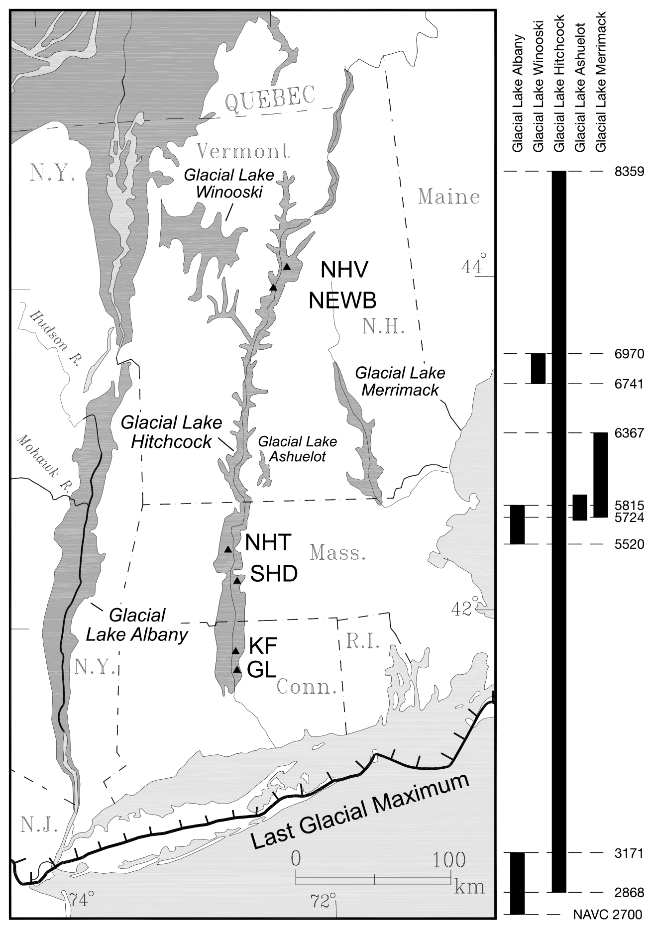
Figure 1Map of New England and adjacent parts of the eastern United States and Canada showing the location and extent of the NAVC (Ridge et al., 2012). The NAVC consists of sediments from several proglacial lakes that existed at different times. The dark shaded areas show the maximum extent of major proglacial lakes present during deglaciation, although lake boundaries were time-transgressive throughout deglaciation and these do not represent exact lake boundaries at a specific time. Labeled triangles show the location of sections sampled for this study (the abbreviations follow Table 1), with the exception of 930PN, which is located off the map to the west in central New York. Nearly the entire time span of the NAVC is represented by sediments from Glacial Lake Hitchcock, and sequences from other nearby glacial lakes are correlated with the Lake Hitchcock sequence as shown in the stratigraphic diagram at right. Although lake sediments at any particular point span a range of NAVC years, deglaciation of the area proceeded from south to north, so, in general, younger (higher-numbered) varves are found at more northerly sites (Fig. 2).
Table 1Characteristics and purpose of varves and sets of varves sampled for Be measurement.
* Varves at 930PN are unusual in that they are derived from a limestone source and predominantly carbonate.
Glacial varves in the NAVC are, in general, substantially thicker than paraglacial varves and are derived predominantly from direct glacial meltwater and sediment production, although paraglacial sources including surface runoff from the recently deglaciated landscape adjacent to the lake may contribute. At any one location in the lake, the contribution of paraglacial sediment to glacial varves increases upsection as the distance to the receding ice margin increases. Glacial varves, especially in areas proximal to the glacier, have melt season (summer) layers composed of a stack of micrograded beds that often fine upwards. Summer layers grade into a non-melt season (winter) layer composed of nearly pure clay, 60 % or more of which is typically less than 1 µm in size. Glacial varve sections also occasionally have extremely thick varve couplets (over 50 cm) with single thick graded beds produced by the sudden release of water from proglacial lakes impounded in tributary valleys (see, for example, Thompson et al., 2017). Paraglacial varves are thinner, typically millimeter scale, and composed predominantly of glacial till, outwash, and other ice-marginal sediments that were deposited on the surrounding landscape and subsequently eroded and transported to the lake by surface runoff after deglaciation.
Paraglacial varves in the NAVC are considered to be varves formed with zero or negligible direct glacial input, although the transition between glacial and paraglacial varves is typically gradational. They are composed of silty and fine sandy summer layers, and may have occasional graded fine sand beds much thicker than a typical summer layer that represent unusual runoff or flood events that washed sandy sediment onto the lake floor. Winter layers in paraglacial varves have diffuse contacts with summer layers below and sometimes show single, internal silt to fine sand laminations that may represent fall overturning.
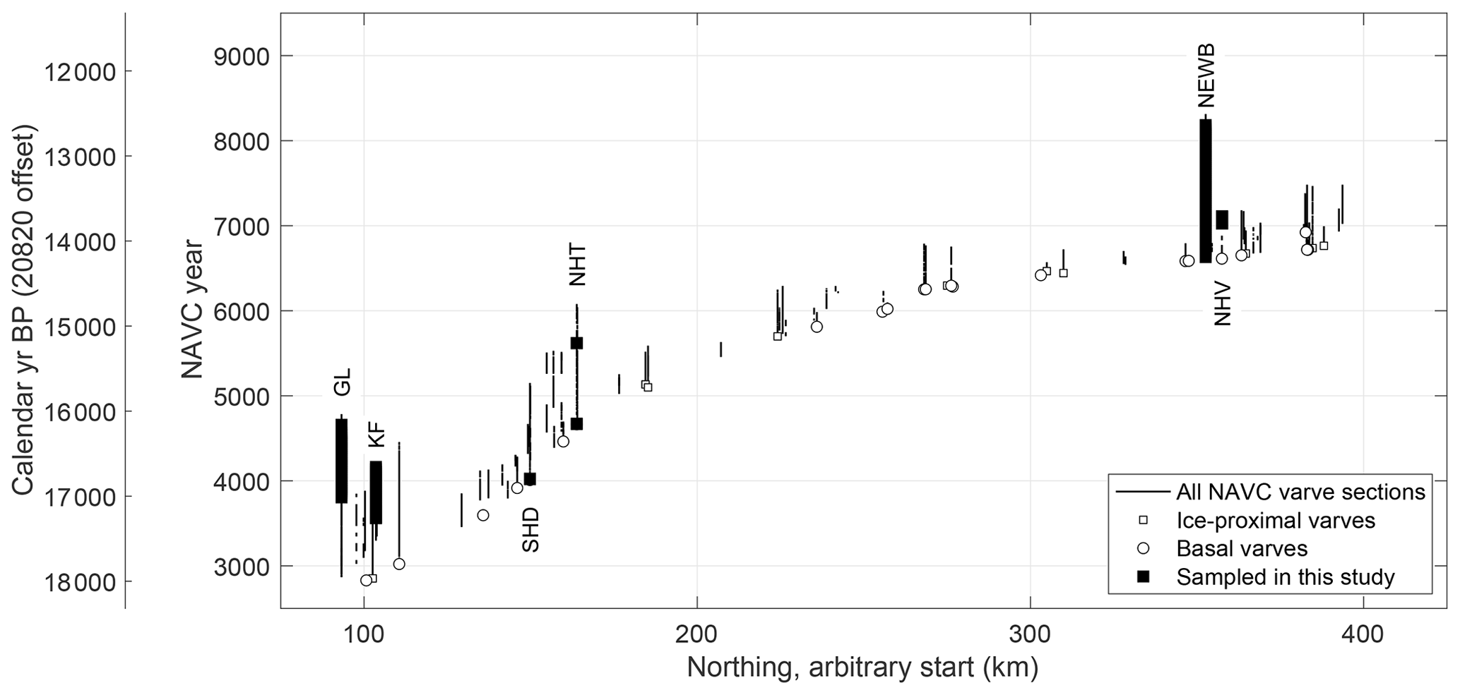
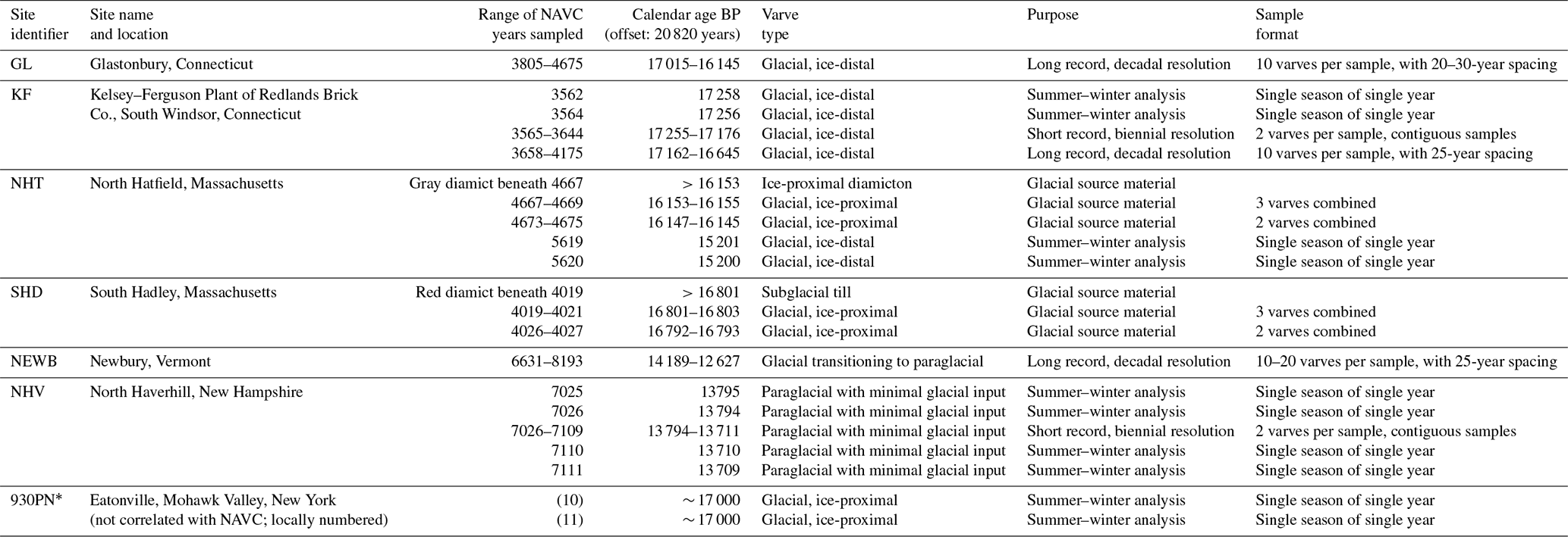
Figure 2Time–distance diagram for NAVC varve sections, highlighting sections sampled in this paper. Thin lines show the age range and location of varve sections in central New England that are correlated with the NAVC. Circles and squares highlight basal or ice-proximal varves, respectively, that indicate the location of the ice margin in a given varve year. Thick lines at labeled sections indicate portions of these sections analyzed in this study. As in Fig. 1, the 930PN section in New York is not shown here. The calendar year BP timescale at left uses the value of 20 820 years for the NAVC year–cal yr BP offset from Thompson et al. (2017); see discussion in Sect. 1.2.
1.2 Existing calendar year calibration of the NAVC
Although the NAVC is continuous for its entire length, the lakes in which varves were deposited drained ∼ 12 000 yr BP, so the varve chronology does not have an absolute connection to the calendar year timescale. The majority of the NAVC that lies near or below the glacial–paraglacial transition is replicated in multiple sections (Fig. 2) and is therefore believed to have zero or negligible counting uncertainty; a number of spurious or missing varves at individual sections have been identified and removed from the chronology (Ridge et al., 2012). The uppermost part of the NAVC consists of thin paraglacial varves that only occur at one section (Newbury; see Figs. 1, 2), and Ridge and Toll (1999) estimated that counting uncertainty in the unreplicated part of the Newbury section above ∼ NAVC 7500 is () years at the top of the section. However, this counting uncertainty is not relevant for the present paper because we will not consider any ice core–NAVC correlations for varves above the glacial–paraglacial boundary. Therefore, if we assume that the NAVC is linear with respect to true calendar years, the calibration of the NAVC to the true calendar year timescale can be represented by a single value for the offset between NAVC years and calendar years. The offset throughout this paper is defined as the age in years BP of NAVC year zero, wherein “years BP” means “years before 1950”, as typically defined for purposes of radiocarbon age calibration. NAVC years are positive and increasing towards the present, and calendar years BP are positive and decreasing towards the present, so the offset is equal to the sum of the NAVC year of any varve and the calendar year BP in which that varve was deposited. Although previous publications (e.g., Ridge et al., 2012; Thompson et al., 2017) variously report estimates for (NAVC–calendar years BP) and (NAVC–calendar years before 2000) offsets, in this paper we use only the NAVC–calendar year BP offset to minimize confusion. Later in this paper, we will also correlate the NAVC with ice core records on the GICC05 timescale (Andersen et al., 2006). Again, throughout this paper we apply the GICC05 timescale in years BP rather than years before 2000 as is sometimes used elsewhere. As the GICC05 timescale is not exactly linear with the true calendar year timescale because of imprecision in ice core layer counting (Adolphi et al., 2018, and references therein), NAVC–cal yr BP and NAVC–GICC05 yr BP offsets may not be exactly the same, and we will use both of these terms as appropriate throughout this paper.
The value of the NAVC–cal yr BP offset has been determined by fitting radiocarbon ages of plant macrofossils associated with individual varves to the INTCAL09 (in Ridge et al., 2012) and subsequently INTCAL13 (in Thompson et al., 2017) calibrated radiocarbon timescales. Thompson et al. (2017), using the INTCAL13 calibration, obtained a best estimate for the NAVC–cal yr BP offset of 20 820 years. The uncertainty in this estimate is not well quantified because residuals between the measured 14C ages and those predicted by the best-fitting offset to INTCAL13 scatter significantly more than expected from measurement uncertainty and are not normally distributed (see discussion in Ridge et al., 2012, and also in Sect. 4.2.4). Ridge et al. (2012) estimated the uncertainty in the calibrated value of the offset to be on the order of ∼ 200 years and also interpreted the distribution of the residuals to indicate that the most likely source of excess scatter was small amounts of sample contamination by postdepositional carbon. If true, this would imply that the true value of the offset is ∼ 100–200 years higher than the 20 820-year estimate.
Both Ridge et al. (2012) and Thompson et al. (2017) proposed that the estimate of the NAVC–cal yr BP offset could be further refined by aligning prominent climate variations evident in Greenland ice core records with changes in varve thickness and/or ice margin position recorded in the NAVC. For sections of the NAVC near 14 000 yr BP, this alignment yielded a NAVC–GICC05 offset of 20 820 years, which is the same as the best-fitting offset inferred from matching 14C data to INTCAL13. This result implies a zero offset between INTCAL13 calendar years and GICC05 years at 14 000 yr BP, which is within the range of existing estimates (Adolphi et al., 2018). For sections of the NAVC between 16 000 and 18 000 BP, their alignment of NAVC and ice core climate proxies yielded a NAVC–GICC05 offset of 20 750 years, which may be consistent with the observation that GICC05 likely undercounts ice layers in the 13 000–20 000 yr BP interval (Andersen et al., 2006; Rasmussen et al., 2008; Adolphi et al., 2018). However, as noted above, radiocarbon calibration of the NAVC still suggests that the NAVC–INTCAL13 offset may be ∼ 100–200 years larger than 20 820 years. In addition, it is important to note that matching variations in NAVC and ice core climate proxy records relies on the assumption that the responses of δ18O variations in Greenland ice cores and varve thickness records in New England to climate changes have similar lag and relative amplitude, which has not been independently established. Also, matches based on these correlations were derived by looking for possible correlations that were close to the NAVC–calendar year offset already estimated from the 14C data. Both ice core and varve records show periodic variability, so multiple matches could be possible in some time ranges.
1.3 Beryllium-10 in lacustrine sediments
Beryllium-10 fluxes to the Earth's surface in polar regions reconstructed from 10Be concentrations in ice cores have been widely used as a proxy for solar variability on interannual to centennial timescales (e.g., Beer et al., 1990; Yiou et al., 1997; Finkel and Nishiizumi, 1997; Steig et al., 1998), and 10Be fluxes to marine sediments have been used to infer paleomagnetic field strength changes on timescales from thousands to millions of years (e.g., Simon et al., 2016, and references therein). By comparison, relatively few studies have attempted to identify solar variability on decadal to centennial timescales using 10Be measurements from lacustrine sediments. Ljung et al. (2007) found that 10Be fluxes recorded in lacustrine sediments deposited between 900 and 1450 CE were similar to those recorded in Greenland ice cores for the same time period. More relevant to this study, Mann et al. (2012) and Czymzik et al. (2016, 2018) measured 10Be concentrations in annually laminated modern and late-glacial sediments, respectively, from European sites and concluded that variability in 10Be fluxes to the lake was attributable to both direct variations in fallout to the lake due to solar variability and variability in environmental factors affecting transport and scavenging of fallout 10Be in the lake. These authors suggested several approaches to accounting for these factors in reconstructing the 10Be fallout flux, mainly focused on multiproxy analysis of lake sediment and the use of multivariate correlation analysis to isolate variability in the 10Be flux that could not be explained by measured environmental proxies. In this work, we attempt to simplify approaches used in those studies by measuring both 9Be and 10Be in lake sediments and applying the following interpretive framework.
Our basic approach is to (i) use 9Be concentrations in sediment as a measure of both the delivery of background Be to the lake and any environmental factors affecting Be scavenging efficiency in the lake and then (ii) identify additional variation in the 10Be flux that cannot be accounted for by these effects and must therefore represent variability in the atmospheric fallout flux. We quantify this with a simple model for Be fluxes to glacial lake sediments. Because we are working with annually laminated sediments, we can directly measure Be fluxes to the sediment (throughout this paper represented in units of ) as the product of the Be concentration in sediment (atoms g−1) and the mass accumulation rate () computed from annual layer thickness (cm yr−1) and density (g cm−3).
We assume that measured Be fluxes to lake sediments derive from one source of 9Be and two sources of 10Be. First, sediment delivered to the lake either from glacial discharge or landscape runoff contains “inherited” 9Be and 10Be. Inherited 9Be includes adsorbed 9Be resulting from subglacial and subaerial mineral weathering. Inherited 10Be could arise from a number of processes, presumably mainly including subglacial recycling of sediment with adsorbed 10Be from a past history of surface exposure and interaction between subglacial sediment and fallout 10Be already present in ice sheet ice. We refer to all Be arising from these sources collectively as “inherited” Be.
Because Be is insoluble and effectively adsorbed to sediment at neutral pH, we expect that sediment delivered to the lake by glacial meltwater discharge will include inherited 9Be and 10Be with a characteristic 10Be∕9Be ratio. The factors controlling the 10Be∕9Be ratio of glacial sediment are presumably complex and include the Be concentration of sediment source material, water–rock interactions in the subglacial environment, the concentration of 10Be in ice, and the rate and extent of basal and surface melting. However, we assume that whatever these processes, subglacial sediment mixing is effective across a significant area of the ice sheet and results in a characteristic 10Be∕9Be ratio in subglacially discharged sediment that can be assumed to be constant, or at least slowly varying, over the 100- to 1000-year timescales represented by our sample sets.
Second, once glacial sediment with a characteristic 10Be∕9Be ratio is delivered to a proglacial lake, additional 10Be can be supplied to the lake from atmospheric fallout and adsorbed to the sediment during transport or deposition, but 9Be cannot. Thus, Be in lake sediment includes inherited 9Be, inherited 10Be, and fallout 10Be.
With these assumptions, Be concentrations in lacustrine sediment (which we can measure) can be related to the flux of atmospheric fallout 10Be (which we seek to reconstruct) by
where Q10,T is the total 10Be flux () to the sediment, which is the product of the measured 10Be concentration (atoms g−1) and the mass accumulation rate (); Q9,T is the corresponding total 9Be flux (; calculated in the same way as Q10,T); Q10,A is the flux of atmospheric fallout 10Be to the surface (); RS (nondimensional) is the characteristic 10Be∕9Be ratio of sediment supplied to the lake; and f (nondimensional) is a focusing factor. The two terms on the right-hand side of the equation represent the two possible sources of 10Be described above: inherited 10Be (Q9,TRS) and fallout 10Be (Q10,Af).
The focusing factor f reflects the fact that 10Be deposition occurs throughout the lake and perhaps an adjoining watershed on the ice sheet and/or the surrounding ice-free landscape, whereas sediment deposition only occurs in a fraction of the lake basin. Thus, in area-normalized units (), the deposition rate of fallout 10Be to lake sediment (Q10,Af) is greater than the fallout rate from the atmosphere (Q10,A) to the watershed. The focusing factor depends on the geometry of the lake and its watershed; for example, Ljung et al. (2007) estimated f≃20 for a small lake, Belmaker et al. (2008) estimated f≃15 for the much larger Lake Lisan, and the results of Aldahan et al. (1999) implied f≃3 for the still larger Lake Baikal. Absent significant changes in the geometry of the lake and watershed, however, f is expected to be constant or changing slowly, so because we are interested in the short-term variability of the atmospheric fallout flux rather than its absolute value, it is sufficient for our purposes to estimate the quantity Q10,Af. Therefore, given the framework of Eq. (1) and measured total 9Be and 10Be fluxes to the sediment, the primary obstacle to reconstructing atmospheric fallout fluxes of 10Be is the need for an estimate of RS, which we discuss in detail later from the perspective of analyzing each of our data sets.
The purpose of the model described by Eq. 1 is to separate environmental effects influencing the delivery of Be to the lake from variations in 10Be fallout to the lake and watershed. If the assumptions of the model and the estimate of RS used in applying it are correct, variations in Q10,Af reconstructed by this method should correctly represent variations in fallout and not in Be transport processes. However, the model is very simple and several complications may be relevant for our data. One is that RS and f will likely change over time due to (i) retreat of the ice margin that results in an increase in the proportion of sediment supplied by the deglaciated portion of the watershed, (ii) changes in ice-marginal drainage, and eventually (iii) reduction in glacial meltwater and sediment supply in the transition from a glacial to a paraglacial lake. As noted above, however, it is likely that these changes will either be steady, gradual changes associated with ice margin retreat from the lake basin or large instantaneous changes associated with lake inlet or outlet switching or reconfiguration of ice-marginal drainage. It appears unlikely that these processes would be manifested as periodic decadal- to centennial-scale variations that might mimic the solar variability we seek to identify. A second complication is the possible role of watershed processes; if fallout 10Be were sourced from a significant ice-free watershed surrounding the lake, variations in 10Be fallout rates might be buffered by water–soil interactions in the watershed and reduce observed fallout variability in the lake (e.g., Czymzik et al., 2016). Finally, the potential importance of 10Be already present in ice sheet ice that could be released by surface melt is unknown. The expected contribution from typical 10Be concentrations in ice sheets (order 104 atoms g−1) at moderate melt rates averaged over the ablation zone (order 10 cm yr−1) would be small (order 105 ) compared to the atmospheric fallout flux (order ∼ 1.5×10⁶ ; see Graly et al., 2011). On the other hand, if melt rates averaged over the contributing ablation area reached meters per year, which could be possible during periods of rapid retreat, this contribution might be significant.
2.1 Sample collection
We collected several sample sets from a total of seven varve sections, with various sampling strategies designed to address different aspects of the study (Table 1 and discussion below). Samples were extracted from (i) short cores collected from surface outcrops by cleaning outcrops and driving in short (typically 0.6 m) sections of PVC pipe with a steel cap and sledge hammer as well as from (ii) deep (up to 50 m), continuously sampled hollow-stem auger cores collected in 2007–2009. Cores are archived at Tufts University. All cores were split after collection and partially dried to improve visual identification of layers and facilitate sampling of individual varves. Only cores with minimal coring deformation were sampled. We sampled winter and summer layers of single varves, complete single varves, and continuous sets of contiguous varves by scraping core surfaces and cutting interior sections of the cores to remove any possible surface contamination, then separating varves along partings between layers and scraping top and bottom surfaces to isolate the varve(s) of interest. Each sample was a column or wedge cut such that the cross-sectional area was constant for all varves incorporated in the sample. As in previous work relating to the NAVC (Ridge et al., 2012), we consider a single varve to extend from the bottom of the coarse-grained summer layer to the top of the fine-grained winter layer.
2.1.1 Short biennial records
At two sites, one with glacial varves (the Kelsey–Ferguson, or KF, section; Figs. 1, 2; Table 1) and one with paraglacial varves (the North Haverhill, or NHV, section; Figs. 1, 2; Table 1), we collected continuous sets of samples spanning 80-year periods at 2-year resolution. The purpose of these sample sets is to determine whether decadal-scale solar variability, specifically the ∼ 11-year Schwabe cycle, can be identified in 10Be fluxes to NAVC sediments (see Sect. 4.1 below).
2.1.2 Long decadal records
At two sites, we collected sets of samples designed to produce records of 10Be deposition over 1000–1500-year periods with decadal (ca. 25-year) resolution that could potentially be correlated with 10Be records from ice cores (see Sect. 4.2 below). One set of samples is from glacial varves at the Kelsey–Ferguson (KF) and nearby Glastonbury (GL) sites in central Connecticut (Figs. 1, 2; Table 1) that overlap and together span NAVC years 3658–4675. The second set is a sequence of glacial grading into paraglacial varves from Newbury, Vermont (NEWB; Figs. 1, 2; Table 1), that spans NAVC years 6631–8193.
2.1.3 Winter–summer pairs
To investigate the seasonal distribution of Be deposition, we separately analyzed winter and summer layers from individual varves at four sites (Figs. 1, 2; Table 1): (i) glacial varves from the Kelsey–Ferguson (KF) site; (ii) paraglacial varves from North Haverhill (NHV); (iii) glacial varves at a site in North Hatfield (NHT), MA; and (iv) glacial varves from a section in the Mohawk Valley of central New York (930PN) that is not correlated with the NAVC but was deposited approximately 17 000 yr BP. Varves at 930PN are unusual among NAVC sites in that their parent material is limestone, so they are mostly carbonate.
2.1.4 Ice-proximal sediment and underlying till
To investigate inherited Be concentrations in subglacial sediment that serves as the parent material for varved lake sediments, we analyzed basal ice-proximal varves and underlying diamicton at South Hadley (SHD) and North Hatfield (NHT), MA, from hollow-stem auger cores that penetrated the base of these varve sections. The basal varves are relatively coarse, 2–6 cm-thick varves deposited at the bottom of these sections, presumably close to the ice margin. The diamicton at SHD is a stony subglacial till, whereas that at NHT mixes till and glaciolacustrine sediment and likely represents a subaqueous debris flow near the ice sheet grounding line.
2.2 Grain size measurements
We measured grain size distributions for all samples using a combination of mechanical sieving (for grain sizes larger than 4 Φ) and pipette analysis for smaller grain sizes (e.g., Lewis and McConchie, 2012). Throughout this paper we represent grain size using the logarithmic phi scale of Krumbein (1934), which is commonly used in sedimentology: Φ is the negative base-2 logarithm of the grain diameter in millimeters, so larger values of Φ represent smaller grain sizes. We halted the pipette analysis at 11 Φ (∼ 0.5 µm), but significant fractions (up to 60 %) of all samples were finer than this (Fig. 3). Thus, to calculate mean grain size and sorting parameters (see, e.g., Boggs, 2014) that require the complete distribution, we fit a lognormal distribution to the observed data for each sample and used the fitted lognormal distribution to compute mean grain size and sorting (Fig. 3).
Figure 3Grain size and sediment density measurements. (a) Measured cumulative grain size distributions for summer layers (red), winter layers (blue), and complete single or multiple varves (gray). Pipette analysis stopped at 11 Φ. (b) Example of extrapolating measured grain size data for a representative sample (NAVC 7068-69 from the NHV section) using a fitted lognormal distribution. (c) Relationship between sediment dry density and grain size. The linear approximation shown by the black line (which is fit to all data excluding three low outliers that likely result from failure to completely fill the reference volume with stiff glacial sediment) is used in subsequent flux calculations.
2.3 Sediment density
Measurements of sediment density are required to interpret a Be concentration by weight (atoms g−1) as a Be flux to the sediment (). We measured the dry density of representative samples of glacial varves at the Kelsey–Ferguson (KF) site, paraglacial varves from the North Haverhill (NHV) site, and separate summer and winter layers from North Hatfield (NHT) by pressing a cylinder of known volume into wet sediment and drying and weighing the resulting sample (Fig. 3; Table S2 in the Supplement). This procedure has several potential sources of inaccuracy, primarily due to the stiff and friable nature of the sediment, which causes difficulty in completely filling the standard volume without deforming or compressing the sediment or introducing voids. It is important to note that the purpose of this study is to identify variations in Be flux to the sediment, not to make an accurate estimate of the absolute flux, so from this perspective inaccuracies in density measurements are not necessarily significant. On the other hand, if we assumed a constant density when, in fact, periodic variations in density were present, we could infer spurious Be flux variations. Density variations, in turn, are most likely to be the result of variations in grain size and therefore in porosity and the relative proportion of silt and clay, and our measurements show this effect (Fig. 3). Thus, for subsequent Be flux calculations we compute the density of all samples from mean grain size measurements using the linear relationship shown in Fig. 3, with an uncertainty derived from the standard deviation of the residuals (±0.05 g cm−3).
2.4 Beryllium-9 by ICP-OES
We measured concentrations of adsorbed 9Be using the procedure described in Greene (2016), which involves drying and powdering sediment samples, leaching in 6M HCl for 24 h, then diluting to a suitable concentration for analysis and measuring the Be concentration with a JY Horiba Optima inductively coupled plasma optical emission spectrometer (ICP-OES). Greene (2016) discusses step-leaching experiments and other data used for quality control by assessing the reliability of the procedure. This procedure extracts only adsorbed Be and not structural Be contained in Be-bearing minerals (e.g., beryl). Although the nominal internal precision of the ICP-OES measurement inferred from replicate analysis of liquid standards was typically 1 %–2 %, replicate analyses of splits of the powdered sediment samples showed a total uncertainty of 3.5 %. Thus, we assume that all 9Be measurements have 3.5 % uncertainty.
2.5 Beryllium-10 by accelerator mass spectrometry
We measured 10Be concentrations in sediment samples at the University of Vermont (UVM) using an adaptation of the potassium bifluoride fusion method of Stone (1998). We dried sediment samples, homogenized them by powdering in a Spex shatterbox mill, and subsampled 0.5 g of the homogenized sediment. We mixed the sample with KHF2 and Na2SO4 and spiked the mixture with 0.4 mg of one of several Be carriers prepared from deep-mined beryl and having 10Be∕9Be in the range 2–. We then extracted Be by fusion of the sample, leaching of the fused sample in water, precipitation of excess K as KClO4, and precipitation of Be hydroxide. We modified the published method by adding an ion exchange step in which we redissolved Be hydroxide in dilute HCl, loaded it onto cation exchange resin (Bio-Rad AG50W X8), eluted B and other cations in dilute HCl, recovered Be in 6M HCl, evaporated to dryness, redissolved in dilute HCl, and precipitated Be hydroxide. Finally, we converted Be hydroxide to BeO for Be isotope ratio measurement by accelerator mass spectrometry (AMS) at the Scottish Universities Environmental Research Centre (SUERC) in East Kilbride, Scotland (Xu et al., 2015). For these analyses, we sputtered samples and isotope ratio standards in the ion source for the same amount of time in order to suppress any effect of variations in emittance during sputtering. All 10Be measurements are normalized to the NIST SRM4325 standard material with an assumed 10Be∕9Be ratio of , which is equivalent to the 07KNSTD standardization of Nishiizumi et al. (2007). We processed samples in batches of 16, each containing one process blank and at least one replicate of a sample that was also analyzed in a different batch (see below). The process blank for Be fusion extraction at UVM utilizes a sample of fine-grained fluvial sediment chosen because of its naturally low bulk 10Be concentration and subsequently powdered, homogenized, and etched in dilute HNO3 in a heated sonic bath for an extended period to remove adsorbed Be. We processed 0.5 g aliquots of this material in the same way as the samples. Complete carrier and process blanks contained between 120 000 and 310 000 atoms 10Be, representing 0.1 %–0.7 % of total atoms measured in samples.
In contrast to the leaching procedure used to measure 9Be concentrations, the total fusion method extracts both adsorbed 10Be and mineral-bound 10Be that could result from in situ production of cosmogenic 10Be in any fraction of the sediment that previously experienced surface exposure. However, concentrations of in-situ-produced cosmogenic 10Be are expected to be negligible for the purposes of this study because in situ cosmogenic production rates at moderate elevations (order 10 ) are insignificant compared to deposition rates of atmospherically produced 10Be (order 106 ) and because NAVC sediments are mostly subglacially derived and therefore not previously exposed to the surface cosmic-ray flux. In-situ-produced cosmogenic 10Be concentrations in glacial sediments associated with the Laurentide Ice Sheet, where measured (e.g., Balco et al., 2005), are on the order of 10 000 atoms g−1, which is negligible compared to total 10Be concentrations of order 108 atoms g−1 measured in this study. We therefore assume that the technical inconsistency between our measurements of leachable 9Be and total 10Be is insignificant and disregard it.
To quantify total measurement uncertainty and as a general quality control measure, we prepared large quantities of two representative samples to be analyzed repeatedly throughout the project. The first of these consisted of varves NAVC 3569-3570 from the Kelsey–Ferguson site, collected as part of the 80-year biennial record described above, which we refer to here by the internal UVM sample name BD3. When the BD3 sample was exhausted after 15 measurements, we prepared a second sample for replicate analysis (BD-STAN) by mixing and homogenizing aliquots of several other glaciolacustrine sediment samples from this study. The BD-STAN sample was subsequently analyzed six times.
The purpose of chemical purification of Be for AMS analysis is to produce a sample of BeO that is sufficiently pure to produce a Be ion beam of the same intensity as produced by pure reagent BeO used as an isotope ratio standard. Poor or inconsistent Be yield from chemical purification, or failure to consistently remove contaminants from the BeO target, can result in Be ion beam currents that are low and/or inconsistent compared to those from standards (see Hunt et al., 2008). This is undesirable because (i) low beam currents reduce measurement precision by reducing 10Be count rates, and (ii) inconsistent beam currents can introduce systematic errors in isotope ratio measurements due to current-dependent variations in beam emittance, ion beam transport, or detector efficiency. Although the goal of AMS beamline and detector setup and adjustment is to remove or minimize any beam current dependence of ratio measurements, it is difficult to verify whether this has been achieved for an arbitrarily large range in beam current, so instrument tuning is not a complete substitute for consistent sample preparation.
AMS analysis of Be samples prepared in the first eight chemistry batches showed low and inconsistent beam currents (Fig. 4; mean and standard deviation of sample beam currents relative to standards for these batches were 0.63 ± 0.25). We found that this effect was related to trace Cl remaining in samples after hydroxide precipitation, so we further modified the Be extraction procedure by redissolving Be hydroxide in dilute HNO3 and reprecipitating. Be beam currents from samples in 17 chemistry batches after this modification were higher and less variable (Fig. 4; mean and standard deviation of relative sample beam currents after the modification were 0.87 ± 0.16).
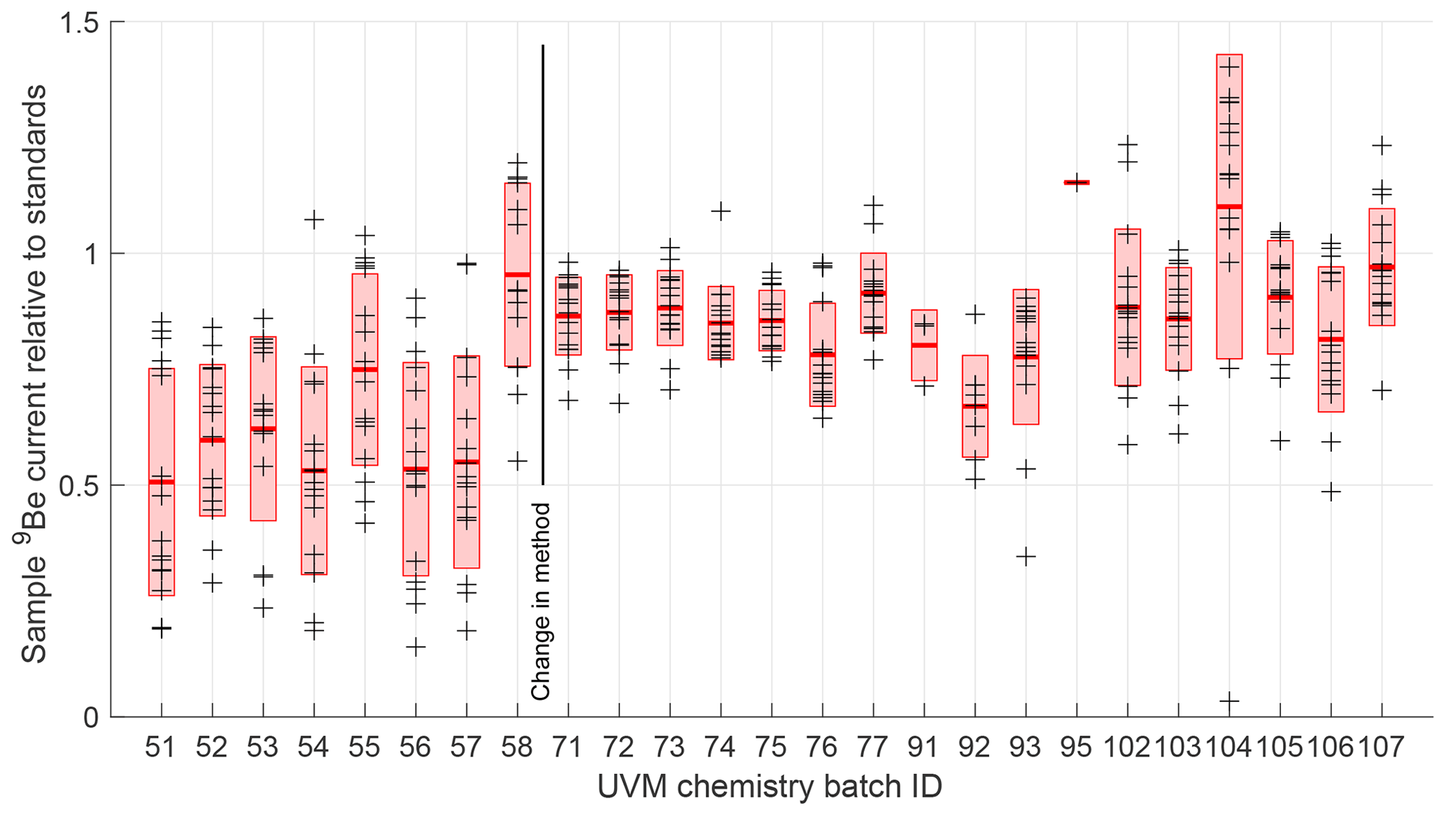
Figure 4Be beam currents during AMS analysis at SUERC relative to Be isotope ratio standards. Each symbol shows the average beam current during analysis of a single sample, normalized to the average current of all primary standards analyzed during the same measurement period. Red lines and pink bars show means and standard deviations for samples processed in each chemistry batch. UVM batch ID numbers are assigned consecutively, so batches are shown in the order they were processed. Only samples of NAVC sediments that are part of this study are included in this plot; some batches included unrelated samples, which are not shown.
Although this change to the sample preparation method significantly improved beam current performance, the complete data set displays high variability in Be currents. Thus, we used the results of replicate analyses, which spanned a range of Be currents, to look for and quantify any beam current dependence in the AMS results. In both replicate analyses and in analyses of groups of samples with similar 10Be concentrations, we observed a relationship between Be beam current and apparent 10Be concentrations derived from AMS-measured 10Be∕9Be ratios (Fig. 5). Although apparent concentrations do not display a significant correlation with beam current for samples with beam currents similar to standards (between ca. 80 % and 110 % of standard currents), our data include a much wider range of beam currents, and when all data are considered, significant correlations are present (Fig. 5). We observed this effect to be persistent through many AMS measurement periods during a 3-year period and similar to the current dependence observed for many replicate measurements of in-situ-produced 10Be in the CRONUS-N quartz standard measured at the SUERC accelerator by Bierman et al. (2017) as well as for analysis of the CoQtz-N quartz standard at an anonymous AMS facility described by Binnie et al. (2019, their Fig. 3).

Figure 5Observed relation between 9Be beam current relative to standards and the measured 10Be∕9Be ratio, here expressed as the nuclide concentration instead of the ratio to account for small differences (ca. 5 %) in sample and Be carrier masses between replicate analyses (see text). (a) 15 replicate analyses of the BD3 sample (see text). (b) Replicate analyses of samples from 80-year biennial records at the KF and NHV sites (see text above); each of these samples was measured at least twice, and light-colored lines connect replicate analyses. Note that true 10Be concentrations vary among samples in this data set, but a significant correlation with beam current is present regardless, and nearly all replicates of individual samples display a positive slope in this diagram. In the left-hand two panels, symbol color-coding indicates the AMS measurement session in which each analysis took place. Sessions 1–2 were measured in 2012, 3–5 in 2013, and 6–9 in 2014. (c) Equivalent data for in-situ-produced 10Be in the CRONUS-N quartz standard (Jull et al., 2015) prepared in the UVM chemistry lab and measured on the SUERC accelerator between 2013 and 2017, as reported by Bierman et al. (2017).
We conclude from these observations that apparent measured 10Be concentrations for our samples that had anomalously low or high AMS beam currents are inaccurate due to beam current dependence of the measured isotope ratios. Lacking a physical model for the observed beam current dependence, we devised the following procedure to correct for this bias. If (C∕CS) is the beam current for a sample relative to the average current for standards measured simultaneously, RM is the apparent 10Be∕9Be ratio observed for the sample, and RC is a nominally correct 10Be∕9Be ratio that would be observed for , then we can define an empirical linear correction factor S such that . In the case in which blank corrections are small to negligible (as is the case for these data; see above) the ratio of apparent and corrected nuclide concentrations NM∕NC, where NM and NC are nuclide concentrations in atoms g−1, is equal to RM∕RC. Thus, to account for small variations in sample and 9Be carrier masses among replicate samples, we correct apparent concentrations instead of ratios using . 0.9 is chosen as the normalizing value because it is the modal value of (C∕CS) for our complete data set, so it minimizes required corrections. Choosing a normalizing value not equal to 1 might introduce a small systematic bias in measured 10Be concentrations relative to the primary measurement standards, but that would not affect any of the results in this study because we are concerned with variability in the 10Be flux and not with a precise measurement of the absolute flux.
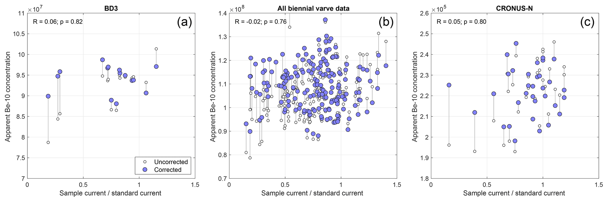
Figure 6Correction for current dependence bias. Uncorrected data shown by open circles are the same data shown in Fig. 5. Corrected concentrations shown by filled circles are connected by light lines to corresponding uncorrected concentrations; error bars are omitted for clarity. For measurements with beam currents comparable to standards, corrections are minimal and similar in size to estimated measurement uncertainties; corrections are most significant for measurements with extreme beam current values. The correlation coefficients and probabilities shown at upper left in all panels are for the corrected concentrations.
We estimate S by choosing the value that minimizes scatter among replicate analyses of the same sample. The sample with the largest number of replicates (BD3; see discussion above) yields S=0.164. The CRONUS-N data of Bierman et al. (2017) yield S=0.185, which highlights the apparent consistency of this effect across multiple samples, chemical preparation methods, and AMS measurement periods. Figure 6 shows the effect of applying this correction procedure with S=0.174 (the average of the above two values) for the data in Fig. 5. Corrected data are uncorrelated with relative beam currents. Note that this correction scheme has the property that corrections for measurements with beam currents comparable to standards (C∕CS between ca. 0.8 and 1.1, within which range no significant correlation between the current and ratio is observed) are minimal and comparable to individual measurement uncertainties; corrections only become significant for samples with extreme relative currents. Figure 7 further highlights this point for the 80-year biennial record from North Haverhill (NHV), which was entirely measured in duplicate. The correction procedure improves agreement between the two sets of measurements primarily by correcting a minority of data that were biased low due to anomalously low beam currents without having a significant effect on the majority of the measurements. For the remainder of this paper, we correct all 10Be concentrations for beam current bias using S=0.174. Although presumably this estimate of S has some uncertainty, a formal estimate of the uncertainty is not necessary because, as discussed below, we derive total measurement uncertainties for 10Be concentrations from the statistics of replicate analyses after correction for beam current bias rather than by propagation of errors through the correction process.

Figure 7Effect of current dependence bias correction on agreement between replicate analyses of NHV biennial samples. All data are assigned 4 % uncertainties as discussed below.
Nominal measurement uncertainties on corrected 10Be concentrations include: (i) AMS measurement uncertainties derived from machine stability and counting statistics (∼ 1 %) and replicate analyses of secondary isotope ratio standards during AMS measurement periods (∼ 1 %); (ii) uncertainty in 9Be carrier concentrations (<1 %); (iii) blank uncertainty (<0.2 %); and (iv) uncertainty in S as discussed above (unknown). Combined, these indicate measurement uncertainties no less than 1.5 %–2 % for most samples. Scatter in measured 10Be concentrations in replicate aliquots of homogenized sediment samples, however, is significantly higher, which indicates that propagation of known uncertainties would underestimate the true measurement uncertainty. Figure 8 shows the reproducibility of replicate analyses of a total of 84 samples. The mean relative standard deviation of all sets of replicate analyses is 4 %, that for BD3 is 3.5 % (for 15 measurements), and that for BD-STAN is 4.1 % (for 6 measurements). We conclude that the true uncertainty in a typical measurement from our sample set is near 4 %, which likely reflects the known measurement uncertainties enumerated above, errors introduced by the correction for current dependence, and imperfect homogenization of sediment samples during preparation. Thus, we compute total uncertainties for all 10Be concentration measurements as follows. First, we assume that each individual measurement has 4 % precision. Second, to incorporate the principle that repeated measurements of the same sample should improve total measurement precision, for samples analyzed more than once, we calculate a weighted mean and standard error (although, as all individual measurements are assigned 4 % uncertainty, they are weighted equally). Summary concentrations and uncertainties calculated via this approach appear in the Supplement and are used henceforth throughout the paper.

Figure 8Relative standard deviation for analyses of replicate splits of 84 sediment samples that were analyzed more than once. Data have been corrected for current dependence bias.
Beryllium-10 concentrations for all NAVC varves (Fig. 9;Table S1) are in the range 0.5–1.5×10⁸ atoms g−1, which is typical of concentrations observed in lacustrine sediments elsewhere (typically 1–10×108 atoms g−1; e.g., Ljung et al., 2007; Czymzik et al., 2016). Total leachable Be concentrations in sediments are 0.6–1.7 ppm, so 10Be∕9Be ratios are in the range 1–. As expected from the inverse relationship between grain size and surface area (e.g., Pavich et al., 1984), the dominant control on adsorbed Be concentrations is grain size: both 9Be and 10Be concentrations are inversely correlated with mean grain size at all sites (Fig. 10). However, 10Be∕9Be ratios are not correlated with grain size, which is important because it supports the hypothesis used in formulating Eq. (1) that inherited Be adsorbed to sediment has a characteristic 10Be∕9Be ratio.
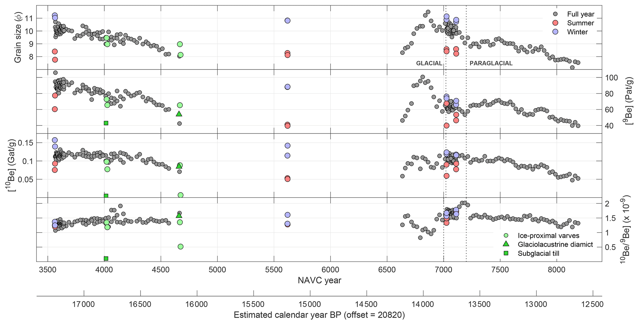
Figure 9Mean grain size and 10Be–9Be concentrations for all samples, shown in stratigraphic order by NAVC year. Seasonal samples from site 930PN, which is not correlated with the NAVC, are not shown. The boundary between glacial and paraglacial varves is between NAVC 7020 and 7200 but is transitional at many sites and also not isochronous between sections. Error bars are not shown for clarity.
Variations in mean grain size, and thus in Be concentrations, at our sample sites reflect a balance of two primary effects. Initially, retreat of the ice margin from a site and therefore an increase in distance from the glacial sediment source will cause an upsection decrease in mean grain size. Subsequently, water depth decreases at the site due to sediment infilling of the lake and glacioisostatic rebound relative to an ice-distal outlet. Shallowing increases the energy of the depositional environment because of increased exposure to surface waves and because the decreasing cross-sectional area of the lake requires that current velocities increase to maintain constant discharge, and it also leads to an upsection increase in grain size. An additional possible effect that may be relevant at some sites is that as the ice margin retreats, sediment is increasingly sourced from the surrounding deglaciated landscape rather than direct ice sheet discharge, and paraglacial runoff sediment is likely coarser than subglacial sediment.
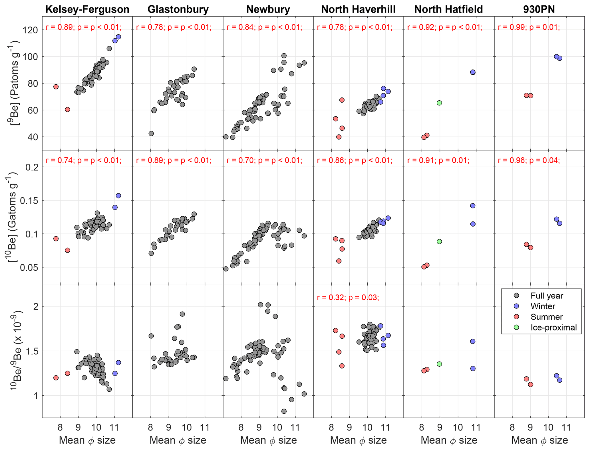
Figure 10Correlation analysis for grain size and Be isotope concentrations and ratio. The correlation coefficient and p value are shown in red when data are correlated at 95 % or better confidence. 9Be and 10Be concentrations are always significantly correlated with mean grain size. However, the 10Be∕9Be ratio is not. Note that Φ size is inverse to dimensional grain size, so a positive correlation between Be concentration and Φ is a negative correlation between Be concentration and grain size.
The long record at Newbury that we sampled with decadal resolution (NAVC 6631–8193; Fig. 9) shows these effects. Grain size decreases and Be concentrations correspondingly increase in the initial part of the record (NAVC 6600–6900) as the ice margin recedes from the site, but subsequently lake shallowing becomes more important and these trends reverse (NAVC 6900–8100). The long records at the Kelsey–Ferguson and Glastonbury sites (NAVC 3658–4669; Fig. 9), on the other hand, begin in relatively ice-distal varves because these sites were deglaciated at about NAVC 2800. Thus, grain size increases and Be concentrations decrease throughout, following the pattern in the upper half of the Newbury section.
Measurements of Be concentrations in separate summer layer – winter layer pairs from individual varves (Figs. 9, 10) highlight the grain size dependence of Be concentrations: finer-grained winter layers have much higher Be concentrations than summer layers, but 10Be∕9Be ratios are not significantly different. In addition, summer and winter data display the same grain size–concentration relationship as full-year data (Fig. 10). Although the winter and summer samples define the end members of the distribution in grain size–concentration space, seasonal and full-year data lie on the same trend.
Samples of ice-proximal glaciolacustrine sediment and underlying diamict (see Sect. 2.1.4) have similar Be concentrations and isotope ratios as more ice-distal glaciolacustrine sediment in similar stratigraphic positions (compare the green symbols in Fig. 9 to other data), with one exception. The exception is a subglacial till (from the SHD section; green square in Fig. 9). In contrast to all other samples, (i) the properties and stratigraphic position of this sample indicate that it has no glaciolacustrine input and has most likely not interacted with lake water, and (ii) this sample has much lower 9Be and 10Be concentrations. Lower Be concentrations are consistent with the relatively large mean grain size (1.1 Φ compared to 8–11 Φ for glaciolacustrine samples, although with much poorer sorting). However, the much lower 10Be∕9Be ratio () in this sample than in glaciolacustrine sediments (∼ 1–; see Fig. 9) is not necessarily expected and may indicate that the majority of inherited 10Be in glaciolacustrine sediments is not reflective of recycling of previously exposed sediment, but it instead may derive from interaction within the subglacial water system between the till and 10Be that is present in ice and released by melting.
4.1 Biennial series
The purpose of sampling two 80-year varve sequences at 2-year resolution is to determine whether or not the 11-year Schwabe solar cycle is present in 10Be flux records. This cycle is evident in ice cores (e.g., Steig et al., 1998) and some lake sediments (e.g., Mann et al., 2012). Recognizing this cycle in the 10Be flux to NAVC sediments would be strong evidence that the NAVC does, in fact, contain a record of global variations in 10Be production and fallout.
4.1.1 Characteristics of biennial series
An 80-year segment of the paraglacial varve sequence at North Haverhill (NHV; Fig. 11) has a mean varve thickness of 0.3 cm, corresponding to mass accumulation rates in the range 0.25–0.75 . As discussed above, 10Be and 9Be concentrations are correlated with mean grain size (Figs. 10, 11). Multitaper spectral analysis (Fig. 11; Dettinger et al., 1995; Ghil et al., 2002) does not show significant spectral power in the 11-year band for any of the observed data series except mean grain size, for which a 12-year peak is significant at 90 % confidence.
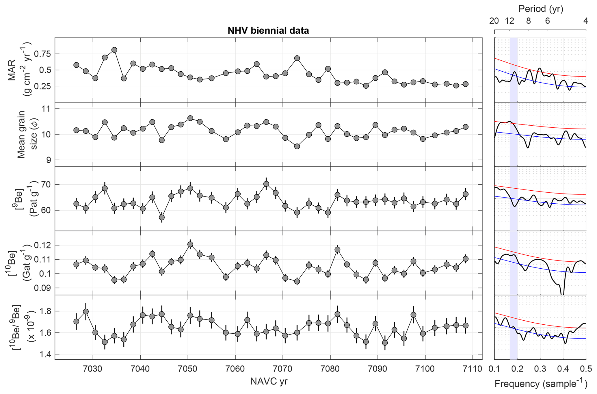
Figure 11Sedimentological data and Be concentrations for an 80-year record with 2-year resolution from paraglacial varves at the North Haverhill (NHV) site. The mass accumulation rate (MAR) is calculated from varve thickness and the density–grain size relationship shown in Fig. 3. Plots at right show results of multitaper method (MTM) spectral analysis of the observational data series using the SSA-MTM Toolkit (Dettinger et al., 1995; Ghil et al., 2002), highlighting frequencies in the vicinity of the 11-year Schwabe solar cycle. Blue and red lines show the 50 % and 90 % significance thresholds, respectively, relative to an AR(1) red noise estimate, and the shaded area highlights the 11-year solar cycle band.
The second 80-year sequence is from glacial varves at the Kelsey–Ferguson (KF) site (Fig. 12) and has a mean varve thickness of 0.85 cm and mass accumulation rates of 0.5–2.5 , more than twice that for the paraglacial varves at NHV. Although all the data from KF (shown in Fig. 10) display significant correlations between grain size and both 9Be and 10Be concentrations, in this subset of the data, 9Be concentrations are significantly correlated with mean grain size (r=0.87; p<0.01) but 10Be concentrations are not (r=0.18; p=0.28). None of the observational data series show significant spectral power in the 11-year band.

Figure 12Sedimentological data and Be concentrations for 80-year record with 2-year resolution from glacial varves at Kelsey–Ferguson (KF) site, with MTM spectra. Plot elements are the same as described in Fig. 11. For the purposes of spectral analysis, missing grain size and 10Be data for two samples were filled by linear interpolation between adjacent measurements.
4.1.2 10Be systematics in biennial series
Be isotope fluxes to the sediment can be derived from the data in Figs. 11 and 12 and are shown in Figs. 13, 14, and 15 for the KF and NHV biennial data. As discussed above, the Be flux (in ) is computed by multiplying Be isotope concentrations (atoms g−1) and mass accumulation rates (). Following Eq. (1), the 9Be flux is inherited 9Be adsorbed to sediment entering the lake, whereas the total 10Be flux includes both inherited and fallout components.
We are interested in reconstructing the fallout 10Be flux (Q10,Af in Eq. 1), and here we attempt to do this by applying Eq. (1) with the following additional assumptions. First, we assume that the inherited 10Be∕9Be ratio RS is constant throughout the time series, which, as discussed above, appears likely over short periods of time. Second, we assume that the fallout flux Q10,Af is variable but approximately symmetrically distributed around a mean value. Although atmospheric production and transport processes are nonlinear with respect to solar variability, assuming a symmetric distribution is likely adequate for short-term variability in the fallout flux that is periodic and has relatively low magnitude. For completeness, we also assume that there is no common forcing of fallout variations and environmental factors affecting 9Be delivery to the lake, which is supported by the fact that Rittenour et al. (2000) did not observe 11-year-band spectral power in NAVC varve thickness records.
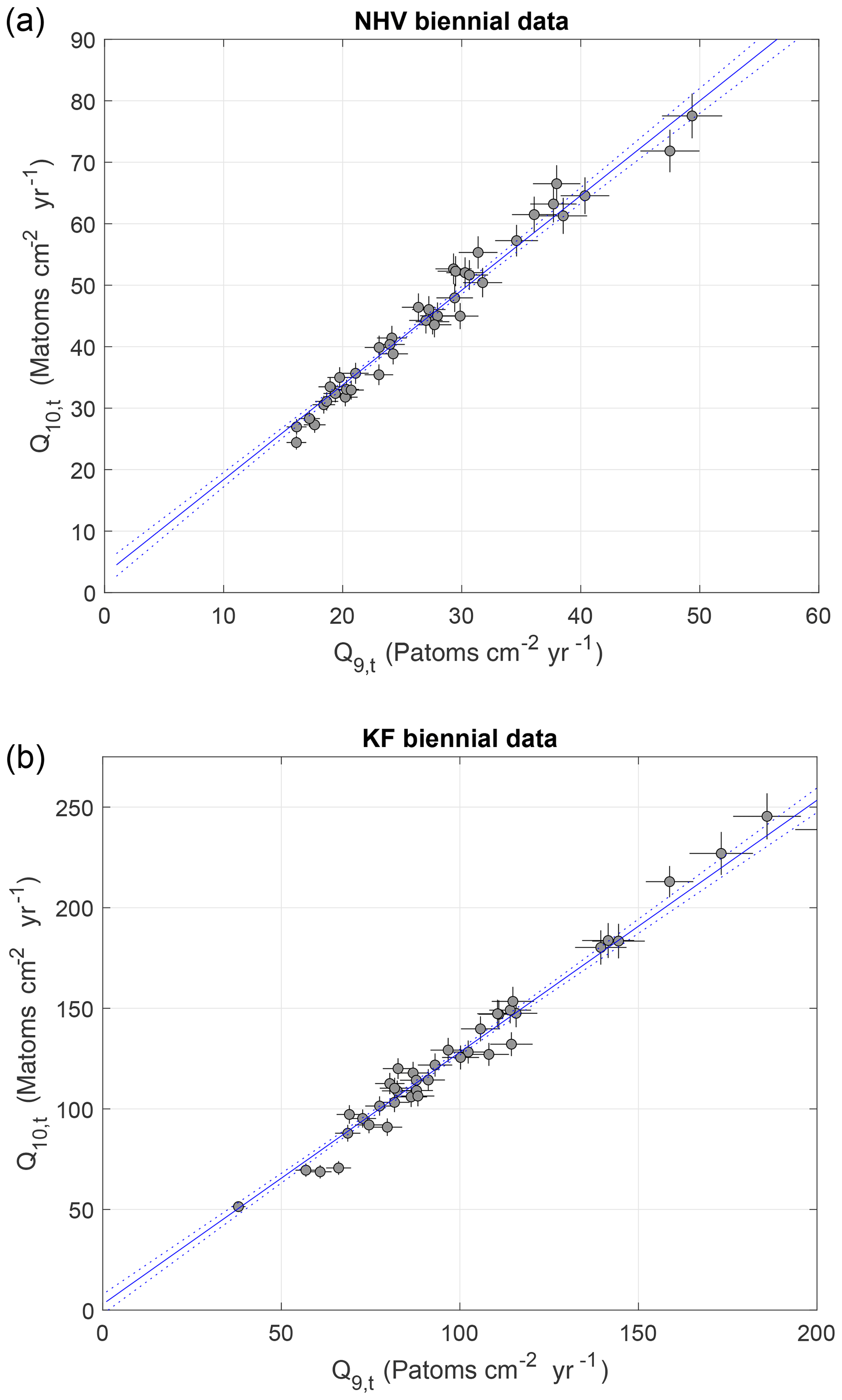
Figure 13Plots showing regression of 10Be against 9Be fluxes for NHV and KF biennial data. Following Eq. (1), the y intercept should give the mean 10Be fallout flux. It is evident that, although this is above zero (as it should be), it is small compared to total 10Be fluxes and comparable in magnitude to measurement uncertainty and scatter around the line. The dotted lines show a 68 % confidence interval for the regression derived from a Monte Carlo simulation.
With these assumptions, Eq. (1) predicts that linear regression of (Q9,T, Q10,T) pairs will yield a line having a slope equal to RS and y intercept equal to the mean fallout flux. Sample-to-sample variation in the fallout flux is expressed as scatter around the line. Q9,T and Q10,T are, in fact, linearly related for both biennial records (Fig. 13). Linear regression for NHV yields and mean(Q10,Af) . The regression for KF yields and mean(Q10,Af) . However, these results imply several complications. First, although intercepts are positive for both data sets, neither are distinguishable from zero at high confidence, and both imply that the fallout 10Be flux is a small fraction (< 10 %) of the total 10Be flux at these sites. This is not favorable from the perspective of reconstructing solar-cycle variability in 10Be fallout fluxes because the expected magnitude of variability in 10Be fallout associated with the 11-year cycle is ∼ 10 %–20 % (Lal and Peters, 1967; Steig et al., 1998). A 10 %–20 % variation in 10 % of the total implies variability in total measured 10Be fluxes no greater than 1 %–2 %, which is smaller than our measurement uncertainties of 3 %–4 %. Second, in agreement with this prediction, Fig. 13 shows that measured 10Be fluxes at both sites are indistinguishable from the regression line at the level of measurement uncertainties. In other words, from this analysis alone we cannot reject the hypothesis that there is zero variation in the 10Be fallout flux and deviations from the linear relationship are entirely due to measurement errors. Both of these observations indicate that relatively high concentrations of inherited 10Be and relatively low concentrations of fallout 10Be result in a poor signal-to-noise ratio for 11-year-period variations in fallout 10Be and a low likelihood of detecting these variations.
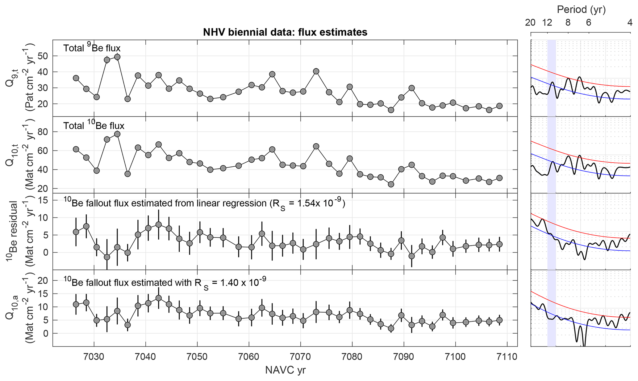
Figure 14Be flux estimates for an 80-year biennial record at NHV. Total fluxes are calculated using the grain size–sediment density relationship shown in Fig. 3. 10Be fallout fluxes are estimated from Eq. (1) using two different values of RS: the value inferred from the linear regression in Fig. 13 and a second value chosen to yield higher apparent fallout fluxes and highlight the fact that apparent time variations in the flux are not strongly dependent on the choice of RS. Error bars reflect the propagation of uncertainty on Be isotope concentrations but not on mass accumulation rates, so it may be underestimated. Plot elements for MTM spectra are the same as in Fig. 11.
Figures 14 and 15 show estimates of the 10Be fallout flux for the biennial data sets using the estimates of RS derived from the linear regressions in Fig. 13. Note that because the scatter of data around the regression lines has a similar magnitude as the mean fallout fluxes estimated from the y intercept, this calculation results in some values for the fallout flux that are less than or indistinguishable from zero. In addition, this calculation yields fallout fluxes that scatter by ∼ 60 % around the mean, which is substantially more than expected for the 11-year solar cycle. These observations suggest that the regression method may be underestimating the 10Be fallout flux. A systematic underestimate might not matter if we are only concerned with whether or not periodic variability exists, but to account for this possibility, we repeated the calculation with values for RS that are lower than inferred from the regressions in Fig. 13 and chosen to yield mean fallout flux estimates that all exceed zero (Figs. 14, 15). Although there is no strong basis for choosing these values, they yield estimates of the 10Be fallout flux that have less relative variability and highlight the property of Eq. (1) that although the choice of RS affects the mean estimated 10Be fallout flux and therefore the relative magnitude of the variability around the mean, it has a minimal effect on its pattern of variability. This, in turn, is important because it implies that an inaccurate estimate of RS is most likely not an obstacle to spectral analysis of short-term variability or correlation with ice core records. On the other hand, the relative magnitude of variability in the reconstructed fallout fluxes is strongly dependent on the assumed value of RS. As our estimate of RS depends on several assumptions and may be unreliable, the magnitude of reconstructed fallout variability is also likely unreliable. This, in turn, is potentially important in evaluating whether or not reconstructed 10Be fallout variations from NAVC sediments are consistent with independent records or with physical limits on the possible variability in atmospheric 10Be production and fallout, and we discuss it in more detail later in Sect. 4.2. From the perspective of the biennial records at NHV and KF, however, this issue is not likely to be relevant because, as highlighted in Figs. 14 and 15, propagated measurement uncertainties in the estimates of the 10Be fallout flux, especially for the paraglacial NHV data, have the same scale as the short-term variability in the estimates. This supports the argument that the unexpectedly large magnitude of short-term variation in the 10Be fallout flux is not the result of incorrectly estimating RS, but indicates that variability in the true fallout flux is smaller than measurement uncertainty in the reconstructed fallout flux and that the majority of apparent variability derives from measurement errors.
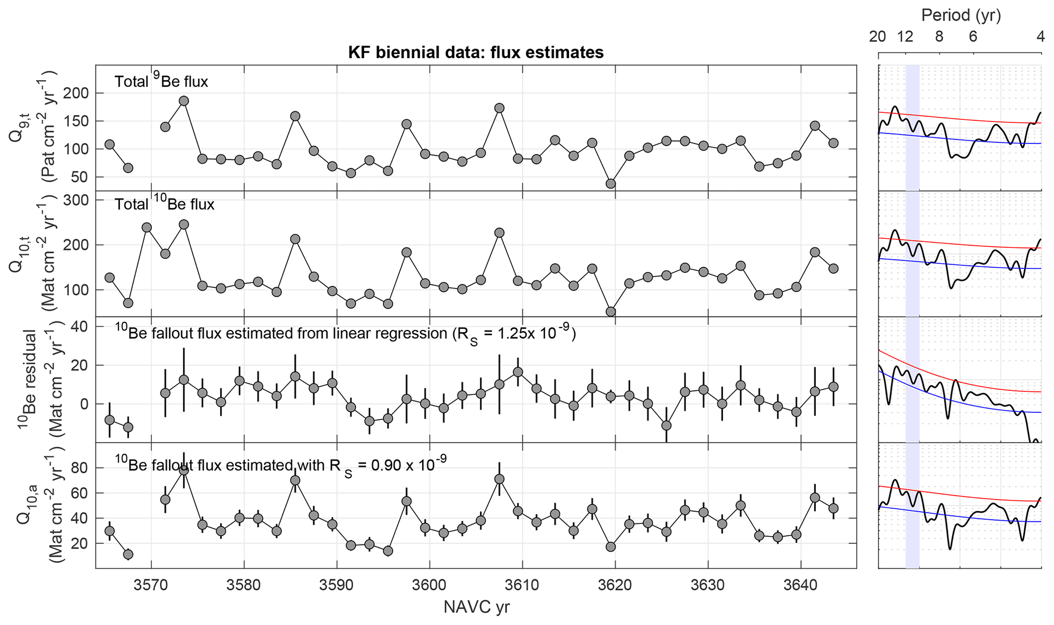
Figure 15Be flux estimates for the 80-year biennial record at KF. Total fluxes are calculated using the grain size–sediment density relationship shown in Fig. 3. Fallout fluxes are estimated from two different assumed values of RS; see text for details. Error bars reflect propagation of uncertainty on Be isotope concentrations but not on mass accumulation rates. Plot elements for MTM spectra are the same as in Fig. 11.
Spectral analysis of reconstructed 10Be fallout fluxes for both biennial records does not display significant spectral power in the 11-year band (Figs. 14, 15). However, results of spectral analysis highlight that the choice of RS has limited importance for spectral analysis of the records; although the significance level of individual peaks varies somewhat with RS, power spectra are similar for different values. For example, RS derived from the regression analysis at NHV (Fig. 14) yields a 14-year peak that is significant at 90 % confidence; a lower value of RS yields the same peak but at lower significance. At KF (Fig. 15), on the other hand, a lower value of RS slightly increases the significance level of peaks in the 10–14-year band.
4.1.3 Summary, biennial series
We conclude from the 80-year biennial records that the 11-year solar cycle can neither be confidently identified nor excluded in these data. In these records, the inherited 10Be flux represents the majority of the total 10Be flux and is much higher than the 10Be fallout flux. Expected variability in 10Be concentrations associated with 11-year-band solar variability is small in relation to measurement uncertainties, which in turn makes it difficult to recognize such variability in 10Be fallout flux estimates derived from our measurements. Spectral analysis did not display significant power in the 11-year band in fallout estimates, but if, as implied by the linear regressions discussed above, true variability in 10Be fallout is smaller than measurement errors in reconstructed 10Be fallout, we would not expect to detect it even if it was present. Therefore, our strategy of using the 11-year solar cycle to test the hypothesis that 10Be fallout variability is recorded in NAVC sediment did not yield a significant result: we have not conclusively proven that 11-year variability is present, but we also showed that, because of the poor signal-to-noise ratio induced by relatively high concentrations of inherited 10Be, we cannot prove that it is absent.
4.2 Decadal series
We now describe results from sampling two ∼ 1000-year varve sequences at decadal resolution. The purpose of these sample sets is to determine whether or not the centennial-scale variability in 10Be fallout fluxes evident in ice core records can be identified in NAVC sediments and, if identified, matched to ice core 10Be records. During some of the time periods represented by these sequences, in particular near 14 000 years ago, ice core 10Be records show centennial-period variations in 10Be deposition with a relative magnitude exceeding 50 %, substantially greater than expected from the 11-year solar cycle. Thus, it is more likely that these longer-period, larger-amplitude variations could be distinguished from measurement noise in NAVC sediments.
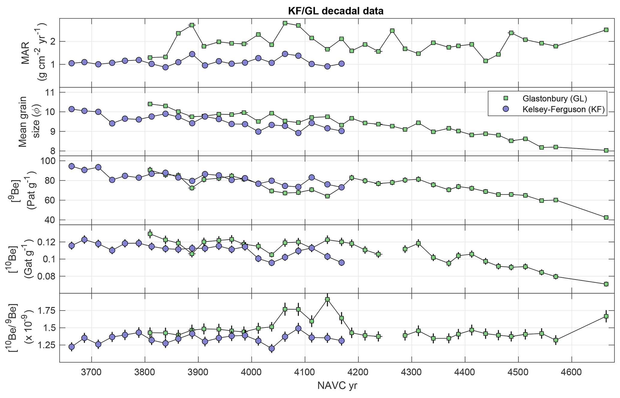
Figure 16Sedimentological data and Be concentrations for decadal-resolution records from adjacent, overlapping sequences of glacial varves at Glastonbury (GL) and Kelsey–Ferguson (KF).
4.2.1 Decadal series of glacial varves from Glastonbury and Kelsey–Ferguson sites
Overlapping sequences of glacial varves from the Glastonbury (GL) and Kelsey–Ferguson (KF) sites in north-central Connecticut (Figs. 1, 2; Table 1; Fig. 16) span NAVC years 3658–4675, approximately corresponding to 17 200–16 200 yr BP. This set of samples has 20–30-year spacing; each individual sample includes 10–15 contiguous varves, and samples collected in the range of overlap of the two sections sample nearly exactly the same varves, although some pairs of samples are offset by 1–2 years. KF is 8 km north of GL and therefore more ice-proximal, but varves at KF are also slightly thinner because the site is shallower and therefore subject to a lower sedimentation rate. The interval sampled was deposited while the glacier was at least 30 km to the north of KF. The mean grain size of matching samples from the same set of varves is coarser at KF, which is consistent with the site being shallower and more ice-proximal (Fig. 16). 9Be concentrations are not significantly different between paired samples, but 10Be concentrations are systematically slightly higher at GL, resulting in 10Be∕9Be ratios that are systematically higher at GL than KF in the period of overlap between the two sample sets.
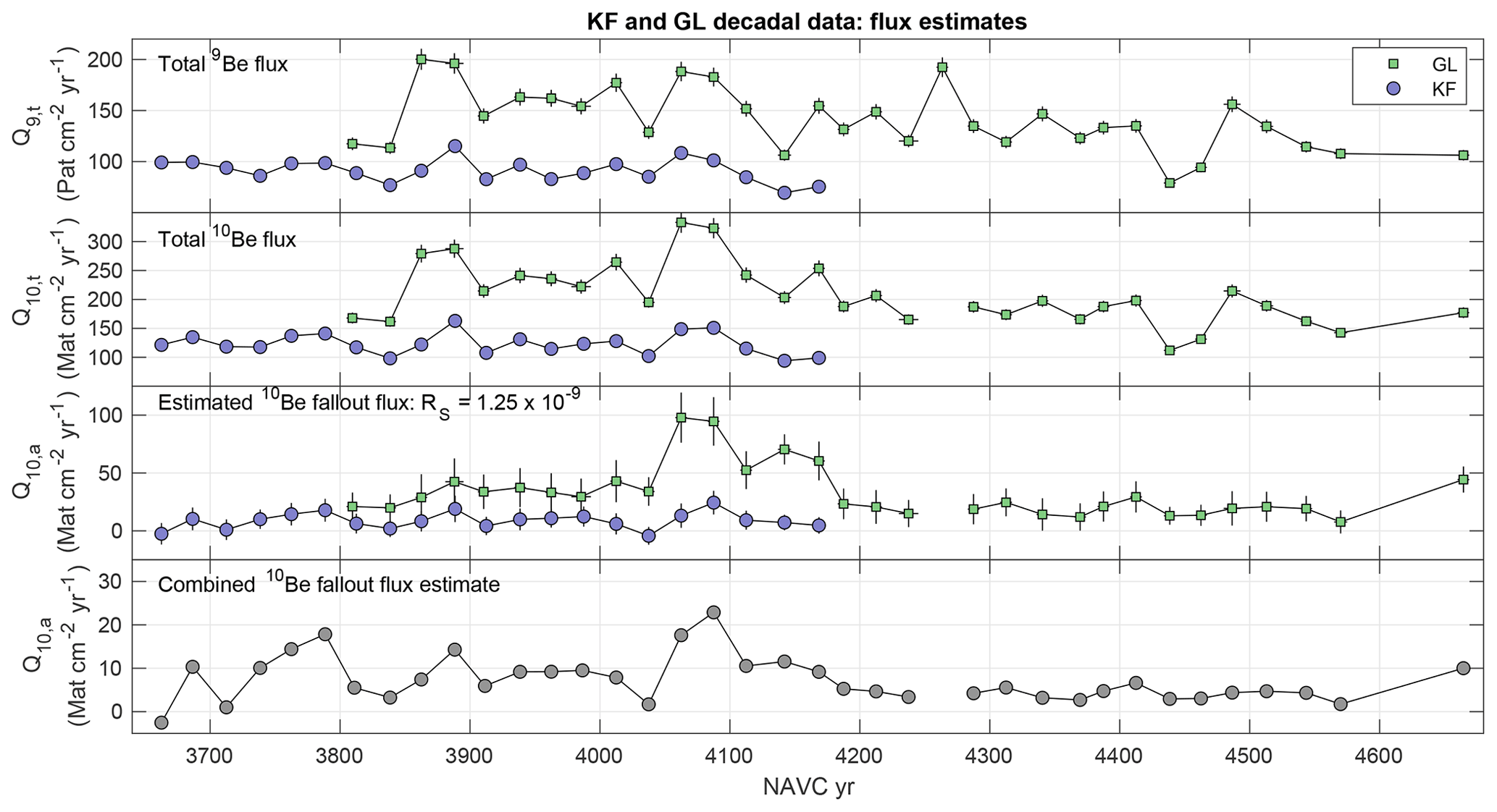
Figure 17Be fluxes calculated for KF and GL decadal records. Upper panels: total 9Be and 10Be fluxes to sediment. Third panel: 10Be fallout flux estimates using Eq. (1) for constant RS. Lower panel: combined estimate computed by linearly scaling the estimate from KF to force agreement in the period of overlap of the two records.
Figure 17 shows estimates of 10Be fallout flux for these sites. When we calculated the 10Be fallout flux for the 80-year records in the previous section, we assumed that RS was constant and variations in the 10Be fallout flux were symmetrically distributed around some mean, which enabled us to estimate RS from linear regression of 9Be and 10Be fluxes. However, for a 1000-year record, these assumptions are not likely to be true. In particular, changes in RS and f are likely to occur on timescales of hundreds of years as the ice margin recedes from a site and the sediment grain size, the size of the contributing watershed, and the balance of glacial and paraglacial sediment all change. In fact, regressions of 9Be and 10Be fluxes for the long records at both KF and GL yield unphysical negative intercepts, which is consistent with the hypothesis that RS is not constant throughout this record.
Thus, lacking any other constraints on RS, we estimated 10Be fallout fluxes using the value of RS that we inferred from linear regression of 9Be and 10Be fluxes for the biennial data at KF as discussed above in Sect. 4.1 (Figs. 17 and 13). The resulting estimates (Fig. 17) have different relative magnitudes, but similar short-term variability, with common excursions around NAVC 3850–3900 and 4000–4100. The fact that reconstructed 10Be fallout variations are similar at both sites could be evidence that we are, in fact, correctly reconstructing true fallout variations. On the other hand, reconstructed fallout fluxes at these sites are weakly correlated with total fluxes, which may indicate that our procedure has not entirely separated environmental and fallout effects on 10Be fluxes. With this value of RS, during the period of overlap of the two records in which flux estimates show limited variability between NAVC 3850 and 4000, the mean estimated fallout flux at GL is near 1×10⁷ , whereas at KF it is near 3.5×10⁷ . Given an approximate average fallout flux for temperate mid-latitudes of 1.5×10⁶ (Graly et al., 2011, and references therein), these imply f≃6 for GL and f≃20 for KF, which are within the range observed for lakes elsewhere. However, as we discussed in Sect. 4.1 with respect to the biennial data, the estimate of RS used to estimate 10Be fallout fluxes affects the mean value and the relative magnitude of reconstructed fallout variations as well as the degree of correlation between total Be fluxes and reconstructed 10Be fallout fluxes, although not the pattern of variability. Thus, although our reconstructed fallout fluxes at these sites imply physically reasonable values for f, it is difficult to conclusively prove from the data themselves that they reflect true fallout variations to the lake system. A systematic difference between fallout fluxes at the two sites could be an artifact of the calculation if RS is not, in fact, the same at both sites, although the fact that the sediment at both sites was sourced from the same ice margin makes this unlikely. Alternatively, it could represent a real difference in the delivery rate of fallout 10Be to the sediment. For example, as GL is farther from the ice margin, the sediment deposited there could have a longer residence time in the lake, which may allow for more complete scavenging of fallout 10Be. If this hypothesis is correct, it could imply that (i) the 10Be fallout flux to the sediment Q10,Af may be quite variable throughout the lake at any given time, and also (ii) variations in sediment transport within the lake could cause variations in the fallout flux at a given site that were unrelated to the actual atmospheric fallout rate. To summarize, our estimates of 10Be fallout fluxes at these sites appear physically reasonable and show reproducible variability in excess of measurement uncertainty, but it is difficult to conclusively prove from the measurements alone that they represent true variations in 10Be fallout to the lake system.
We explored this further by comparing 10Be fallout flux estimates at these sites to coeval ice core records. For the purposes of comparison, we assume that the difference between the two records is most likely explained by differences in f between the two sites and therefore obtain an estimate of centennial-scale variability represented in both records by applying a constant scaling factor to the GL data so as to align the two records where they overlap between NAVC 3810 and 4040, then averaging the two records within the period of overlap. This procedure loses information on the relative magnitude of fallout variability, and our combined estimate has higher internal variability (∼ 50 %; see the bottom panel in Fig. 17) than is observed in ice core 10Be flux records for this time period (∼ 15 %). However, we argued above in Sect. 4.1 that the relative magnitude of our fallout flux estimates is likely unreliable due to its dependence on RS, so it could not be used as a point of comparison with ice core records in any case. Multitaper spectral analysis of this combined record shows a significant (at 95 % confidence) spectral peak at 91 years, which matches a characteristic period observed in solar variability records (the 88-year “Gleissberg cycle”; e.g., Feynman and Fougere, 1984). This, like the similarity of fallout flux estimates from the two records, suggests that variability in our fallout flux estimate is not solely the result of measurement noise and that true centennial-scale variability in 10Be fallout may be recorded.
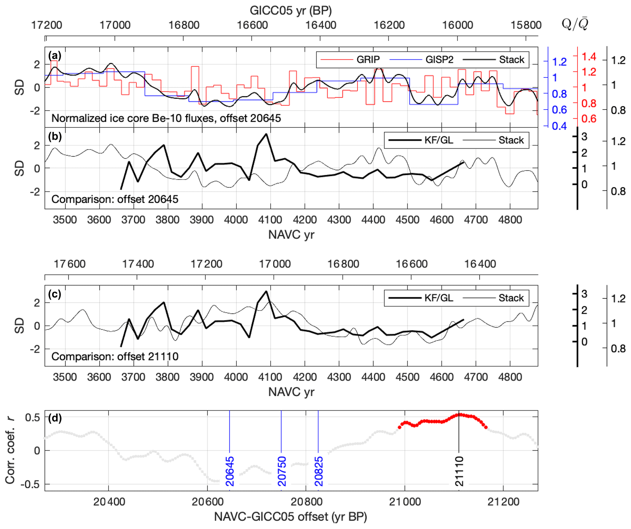
Figure 18Comparison of the combined 10Be fallout flux estimate from the KF and GL sites (Fig. 16) with ice core records of 10Be fallout. (a) Scaled and centered ice core 10Be flux records from Adolphi et al. (2018) (and references therein), offset to NAVC years with a NAVC–GICC05 yr BP offset of 20 645 years (see text). “Stack” is the global ice core stack from Adolphi et al. (2018). (b) Scaled and centered combined KF–GL fallout flux estimate compared to the ice core stack with the same 20 645-year offset. (c) Same as (b), only for an offset of 21 110 years. In panels (a)–(c), because the primary plotted units of standard deviations from the mean obscure the true relative variability of each record, the additional axes at right labeled , which have line colors and weights matching each data series, show units of relative variation with respect to the mean of each data series. This highlights the fact that the apparent magnitude of variations in our reconstructed NAVC fallout flux is greater than expected from coeval variations in ice cores, although, as discussed in the text, this difference could be an artifact of the calculation procedure and we therefore used the scaled records for correlation estimates. (d) Results of correlation analysis comparing the scaled and centered KF–GL fallout flux estimate with the ice core stack. Red highlights values of the offset for which the hypothesis that the two records are uncorrelated can be rejected at 95 % confidence. Vertical lines highlight offsets inferred from radiocarbon dating of NAVC varves (20 820 or 20 645 with the GICC05–calendar year offset of Adolphi et al., 2018, for this time period) and event correlation of varve thickness with Greenland ice core temperature (20825 and 20750; Ridge et al., 2012). All of these yield an inverse correlation between the 10Be records.
Figure 18 compares our combined 10Be fallout flux record to ice core 10Be fallout flux records compiled by Adolphi et al. (2018). Again, as we have argued that the magnitude of variability in our 10Be fallout flux estimate is unreliable, we compare scaled and centered records to focus on the pattern of variability rather than the magnitude. The overall structure of the ice core records in this time period displays periodic centennial-band variability as well as a broader low between ∼ 16 500 and 16 800 GICC05 yr BP. If we start with the NAVC–calendar year BP offset of 20 820 years inferred from 14C data (Ridge et al., 2012; Thompson et al., 2017) and accept the estimate of Adolphi et al. (2018) that the GICC05 chronology is 175 years too young in this time interval, then we expect a NAVC–GICC05 yr BP offset of 20 645. Aligning the composite 10Be fallout estimate from KF and GL with the ice core 10Be stack (Fig. 18b) with a NAVC–GICC05 yr BP offset of either 20 820 or 20 645 does not yield a good match: a peak in the 10Be fallout flux near NAVC 4100 aligns with a period of relatively low flux in the ice core stack, resulting in an inverse correlation between the two records. Ridge et al. (2012), based on correlation between NAVC varve thickness records and Greenland ice core temperatures, suggested NAVC–GICC05 yr BP offsets of 20 825 for events near 16 100 yr BP and 20 750 for events near 17 400 yr BP, and neither of these yields a good match either.
We searched for a better match by looking for the closest alternative value of the offset for which the KF–GL combined fallout estimate is positively correlated with the ice core stack at high confidence (Fig. 18c, d). This occurs for NAVC–GICC05 yr BP offsets in the range 20 965–21 165 years, with the best correlation at 21 110 years. This aligns a series of fallout peaks at NAVC 3700–4100 in the KF–GL record with a broad high around 17 000–17 300 GICC05 yr BP in the ice core records and a period of low variability at NAVC 4200–4600 with a broad low around 16 500–16 800 GICC yr BP. However, the correlation is significant across a 200-year range in the offset, which shows that the correlation analysis is mainly aligning the longer-period structure of the two records rather than the centennial-scale variability. Apparent correlation of ∼ 1000-year-period variations in a record that is only 1000 years long could easily be misleading if the assumption of constant RS and f created a spurious systematic drift.
Overall, our 10Be fallout flux estimate from the KF–GL decadal series (i) shows variations that are reproducible between two sites, (ii) shows evidence for periodic variability in a band characteristic of solar variability, and (iii) shows acceptable correlation with the global ice core 10Be fallout stack using an NAVC–GICC05 offset that is close to the expected value. These observations may suggest that our fallout flux estimate is, in fact, recording global atmospheric 10Be production and fallout variations. On the other hand, the apparent correlation between the two records mostly reflects alignment of long-period variability, which is unlikely to be robust for a relatively short record and in addition could arise from incorrectly assuming constant RS and f. Thus, although this match between NAVC and ice core fallout records is possible and is consistent with the hypothesis that our fallout flux estimate represents true variability in 10Be fallout, it does not provide strong support for the hypothesis.
4.2.2 Decadal series of glacial and paraglacial varves from Newbury
Our decadal-resolution record from Newbury comprises a sequence of glacial varves transitioning to paraglacial varves between NAVC 6630 and 8190 (Fig. 19). This set of samples has 20–30-year spacing, and each individual sample includes 10–20 contiguous varves. Ridge et al. (2012) placed the boundary between glacial and paraglacial varves at NAVC 7100, where relatively thick varves with relatively high interannual variability (high MAR) are overlain by thinner varves (lower MAR) with reduced interannual variability (Fig. 19). However, grain size and Be concentration records (Fig. 19) do not show the same sharp transition, indicating that the glacial–paraglacial transition was more likely characterized by a gradual reduction in glacial meltwater and sediment delivery beginning near NAVC 7100 and continuing for ca. 200 years. Regardless, sediments in the lower part of this section before ca. NAVC 7000 are predominantly derived from direct glacial discharge, and sediments in the upper part after ca. NAVC 7225 are predominantly derived from runoff from the deglaciated landscape. A period of low MAR beginning at NAVC 6800 is associated with the Littleton–Bethlehem Readvance, a period of ice margin expansion into the lake recognized from a moraine complex and related stratigraphic sections ∼ 40 km to the north of this site (Ridge and Toll, 1999; Ridge et al., 2012; Thompson et al., 2017). Although the distance to the ice margin presumably decreased at this time, this effect was offset by reduced meltwater production in a cooler climate that resulted in thinner, finer-grained varves.
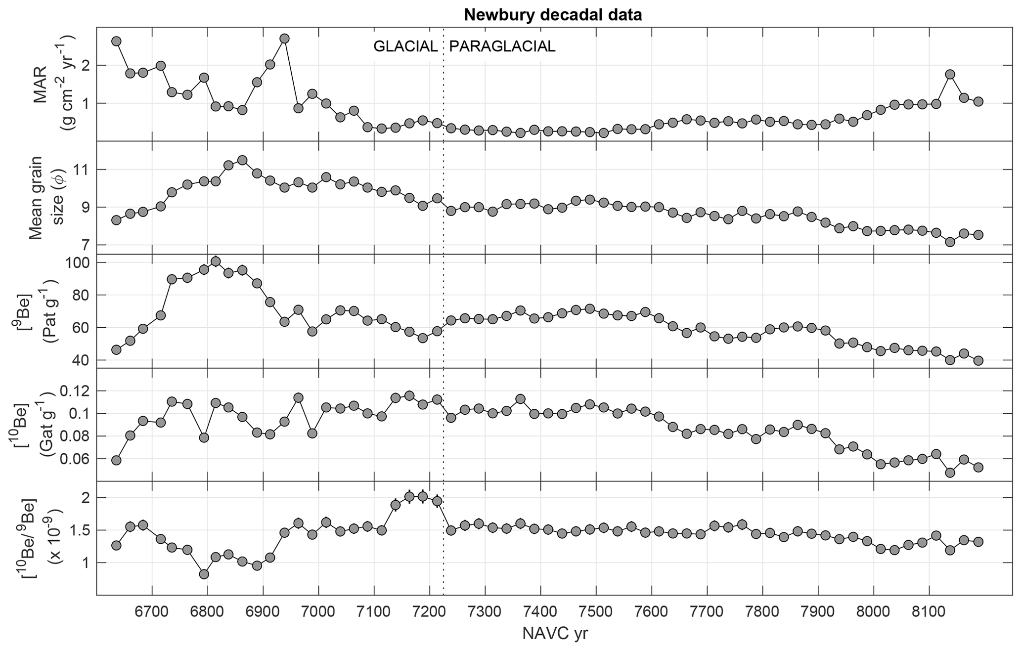
Be isotope systematics are very different in glacial and paraglacial parts of the Newbury section (Figs. 20, 21). Although, as noted above, the assumptions necessary to estimate RS from linear regression of 9Be and 10Be total fluxes are probably not valid for long records, regressions for glacial and paraglacial parts of the section in Fig. 20 differ in a way that is similar to that observed for the paraglacial and glacial biennial records at NHV and KF, and they are consistent with expected changes from a glacial to paraglacial environment. Glacial varves imply and mean(Q10,Af) (e.g., f≃15), and 10Be fluxes display high variability around the regression line, which implies that fallout 10Be represents a significant fraction of the total 10Be flux. Paraglacial varves imply and mean(Q10,Af) (e.g., f≃5), with minimal variability. This is consistent with our hypothesis, discussed above, that RS is expected to be higher for a deglaciated landscape that may have been accumulating 10Be in soils for thousands of years than for direct glacial sediment discharge. The decrease in f between glacial and paraglacial varves at the same site is also consistent with the prediction that f should be larger if the lake watershed includes a significant area of the adjacent ice sheet, so the glacial–paraglacial transition is associated with a significant decrease in contributing area.
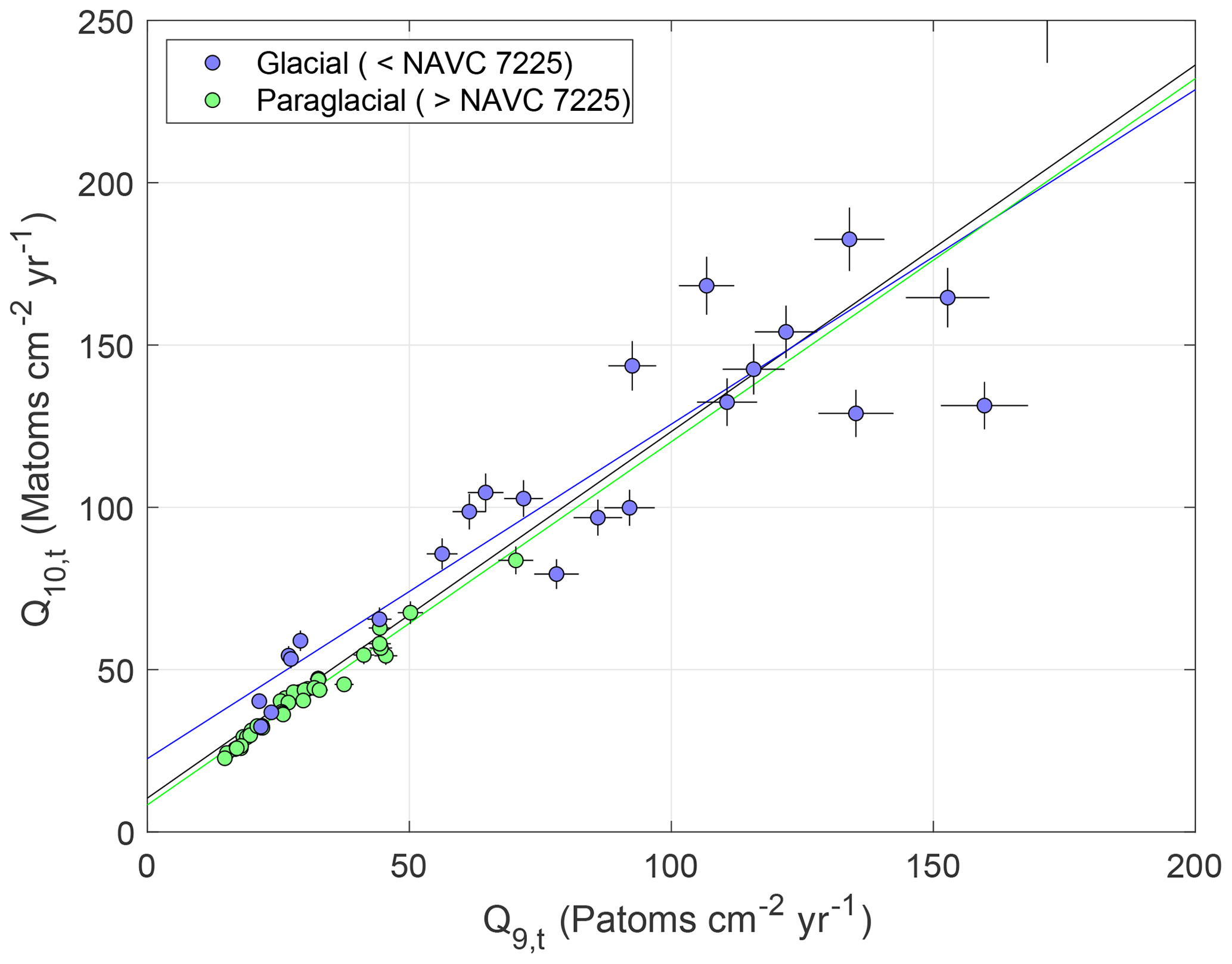
Figure 20Regression of 9Be and 10Be total fluxes for glacial and paraglacial varves at Newbury.
Although this analysis highlights differences in 10Be systematics between glacial and paraglacial varves, application of the estimates of RS from the regression slopes to Eq. (1) would imply unphysical negative 10Be fallout fluxes for several samples. Thus, the estimate of 10Be fallout flux in Fig. 21 uses . Again, the value we assume for RS affects the mean of calculated fallout fluxes and therefore the relative magnitude of the variability but does not affect the pattern of fallout variability.
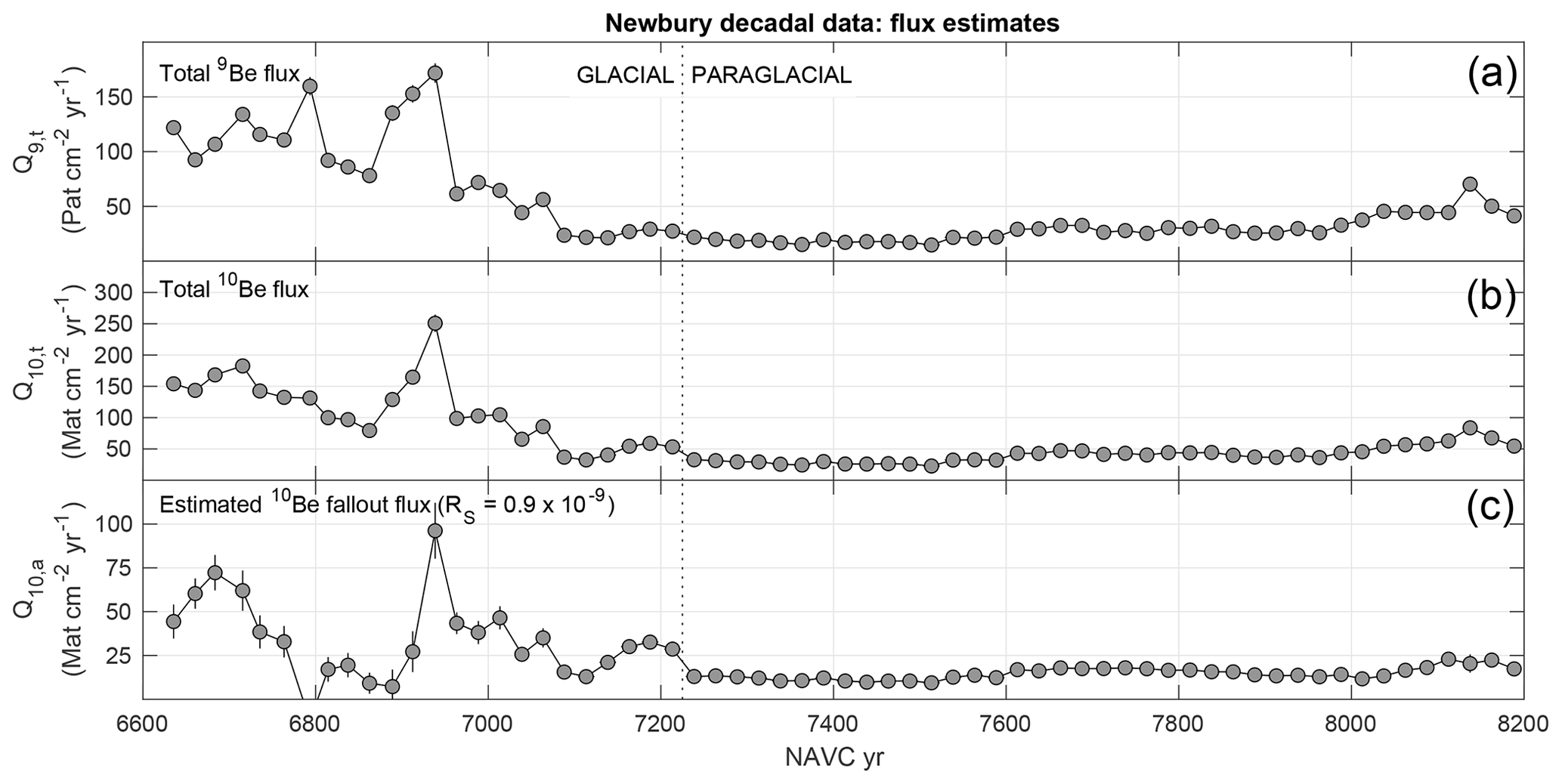
Figure 21Be fluxes calculated for the Newbury decadal record. (a) and (b), total 9Be and 10Be fluxes to sediment. (c), 10Be fallout flux estimate using Eq. (1) for constant RS.
The most striking aspect of 10Be fallout flux estimates for Newbury is that variability in the 10Be fallout flux is strongly suppressed in the paraglacial section. This is a likely consequence of buffering of 10Be fallout by watershed processes in the absence of direct glacial meltwater input. As 10Be is known to accumulate in soils in nearly all environments (Pavich et al., 1984), in a paraglacial landscape, a substantial fraction of 10Be fallout deposited in the watershed is likely adsorbed to developing soils during infiltration and therefore cannot be transported into the lake. Pollen records from this time period show that the landscape was heavily vegetated (Thompson et al., 2017), which highlights the likelihood of rapid soil development and 10Be accumulation in soils in the watershed. On the other hand, 10Be deposited on the surface of an ice sheet with negative mass balance, as presumably was the case for a large extent of the southern margin of the rapidly retreating Laurentide Ice Sheet at this time, cannot accumulate. Fallout 10Be deposited on an ablation area of the ice sheet that drains into a glacial lake must all be flushed into the lake, either by supraglacial or subglacial drainage, during the summer melt season each year. Thus, if a large area of the ice sheet drains into the lake, fallout 10Be from a large area can be effectively concentrated and transported to the lake with a minimal time lag between fallout and delivery. We conclude from the striking contrast between glacial and paraglacial 10Be systematics at this site that glacial lake sediments likely record 10Be fallout variations with a significantly higher amplitude and shorter time lag than paraglacial sediments. Fallout variations in paraglacial lake sediments appear to be strongly suppressed by watershed buffering of 10Be fluxes.
The reconstructed fallout flux in the glacial section at Newbury displays high variability with several peaks that are substantially larger than measurement uncertainty, and it does not show any correlation with total Be flux, so this variability is not likely to be explained by environmental factors. 10Be fallout records from ice cores that are coeval with the Newbury glacial section also display high variability at centennial timescales during this period, and Fig. 22 compares the 10Be fallout flux estimate from Newbury to the ice core records. Note that because the variability in the 10Be fallout flux in the paraglacial section of the record is minimal and near the level of measurement uncertainty, this portion of the record has no effect on a correlation analysis and we do not consider it. The important feature of the ice core records in this time interval is a group of prominent peaks in 10Be fallout that occurred between 13 900 and 14 500 GICC05 yr BP, which are well in excess of the characteristic variability of the surrounding time period. If we accept the estimate of Adolphi et al. (2018) that the INTCAL13 and GICC05 timescales are equivalent in this interval, the best-fitting radiocarbon calibration of the NAVC (Thompson et al., 2017) would imply a NAVC–GICC05 yr BP offset of 20 820 years. Event matching between varve thickness records and ice core climate records in the time range covered by the Newbury glacial section by Ridge et al. (2012) suggested a NAVC–GICC05 yr BP offset of 20 825 years. However, these values fail to align peaks in the varve and ice core 10Be fallout records (Fig. 22) and, in fact, yield an inverse correlation between the two records. In contrast, a NAVC–GICC05 yr BP offset near 20 950 years aligns significant peaks at NAVC 6950 and 6700 with corresponding peaks in the ice core record at 13 975 and 14 300 yr BP (Fig. 22). An offset of 20 925 yields the best alignment of the peaks at NAVC 6950 and 13 975 GICC05 yr BP (the peak at NAVC 6950 dominates a correlation metric; see Fig. 22), but a value of 20 950 better aligns both peaks (as the Newbury record has 25-year spacing, the difference between 20 920 and 20 950 is not significant). Other matches are possible because the Newbury record displays two major peaks and the ice core records display three major peaks with several adjacent minor ones in this time period. For example, an offset near 20 675 would align the peak at NAVC 6700 with the peak at 13 975 BP.
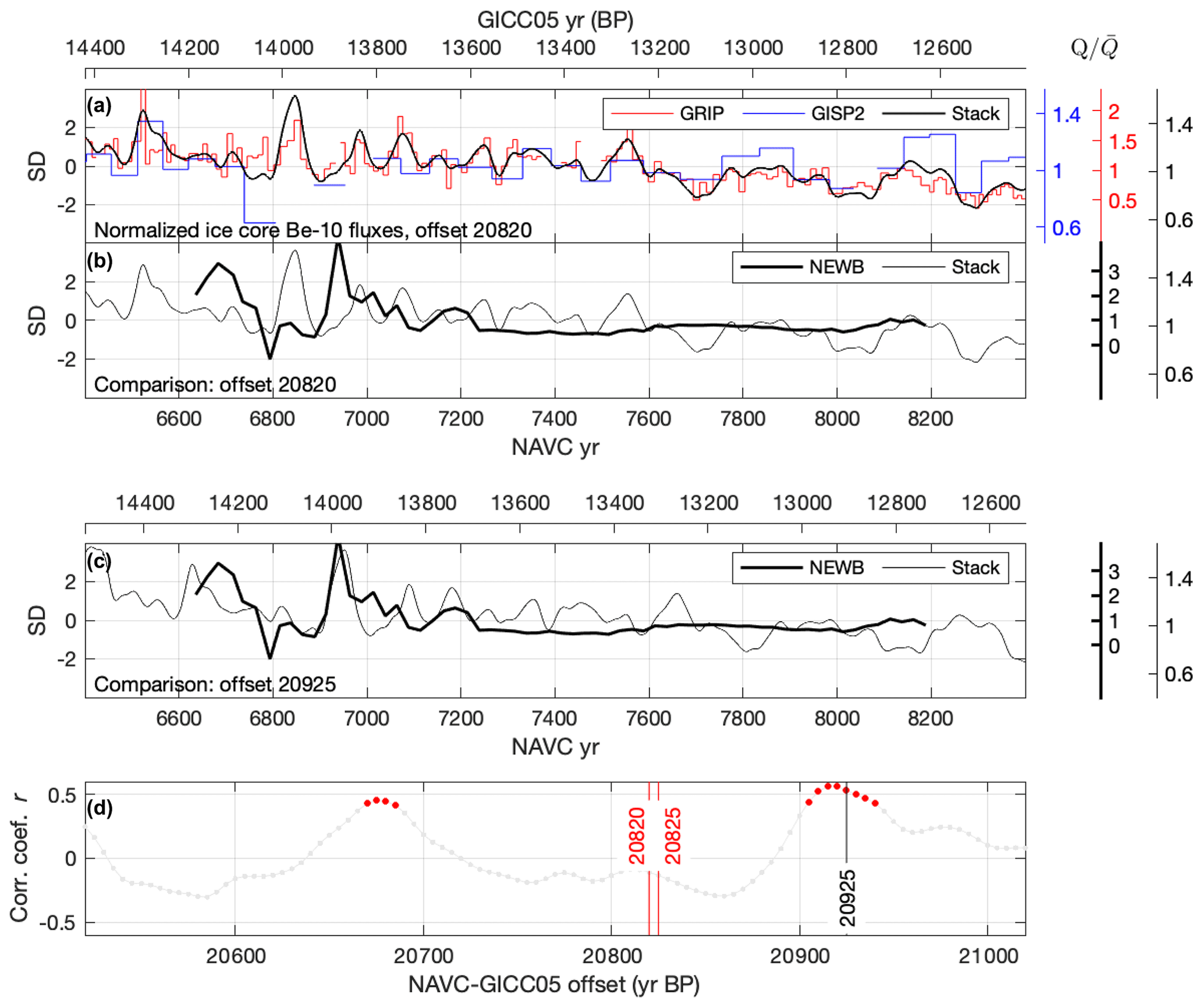
Figure 22Comparison of the 10Be fallout flux estimate from Newbury with ice core records of 10Be fallout. Plot elements are the same as in Fig. 18. (a) Scaled and centered ice core 10Be flux records from Adolphi et al. (2018), offset to NAVC years with the value of the offset inferred from 14C data (Thompson et al., 2017) and the assumption that INTCAL13 and GICC05 timescales are equivalent in this interval. (b) Scaled and centered Newbury fallout flux estimate compared to the ice core stack for the same offset. (c) Same as (b), only for an offset of 20 925 years that aligns peaks in varve and ice core 10Be (see text). As described in the caption to Fig. 18, the additional axes to the right of panels (a)–(c) show units of relative variation with respect to the mean of each data series. (d) Correlation between varve and ice core 10Be records for different offset values. This considers only the glacial part of the section; the minimally variable paraglacial section does not affect the conclusions. Vertical lines highlight other suggested offsets inferred from radiocarbon calibration (20 820) and event correlation (20 825; see text).
Overall, the most prominent feature of the decadal-resolution 10Be record at Newbury is the strong contrast between 10Be systematics in glacial and paraglacial varves. This, as argued above, indicates that 10Be fallout variability is likely to be enhanced in glacial varves by 10Be runoff from the ice sheet but suppressed in paraglacial varves by watershed buffering. The glacial part of the section displays significant centennial-scale variability in reconstructed 10Be fallout, which can be acceptably correlated with coeval ice core records using values for the NAVC–GICC05 yr offset that are close to those inferred from other evidence.
4.2.3 Decadal series, summary results
Although the paraglacial section at Newbury does not show significant variability in 10Be fallout flux, 10Be fallout flux estimates from the glacial sections at Newbury, Kelsey–Ferguson (KF), and Glastonbury (GL) display variability in excess of measurement uncertainty that can be correlated with global ice core 10Be fallout records using NAVC–GICC05 yr BP offsets that are similar to independently estimated values. Despite several unverified assumptions in our reconstruction of 10Be fallout fluxes from Eq. (1) and significant uncertainties in relating the apparent magnitudes of 10Be fallout variability to those expected from global records, these observations are consistent with the hypothesis that apparent 10Be flux variations in NAVC sediments are, in fact, recording true fallout variations.
The NAVC–GICC05 yr BP offsets that produce the best matches at Newbury and KF–GL are different, in the range 20 900–20 950 for Newbury and 20 965–21 165 at KF–GL. The match with Newbury is substantially more likely to be valid because it is based on aligning anomalously large, short-duration peaks in both records that are expected to be insensitive to possible longer-term variations in RS or f, whereas the apparent match for the KF and GL sections is not well defined and could be a result of assumptions in the fallout calculation. In general, estimates of the NAVC–GICC05 offset obtained for different time ranges are not required to be the same because the GICC05 timescale is not exactly linear in calendar years (Adolphi et al., 2018). If the apparent matches at Newbury and KF–GL were both valid, the difference would imply that GICC05 is overcounted by ∼ 150–200 years between 14 000 and 17 000 BP. However, other estimates of the GICC05–calendar year offset (Adolphi et al., 2018, and references therein) show the opposite, that it is undercounted by ∼ 175 years during this interval, so a GICC05–NAVC offset of 21 000 for KF–GL should be equivalent to an offset of 21 175 at Newbury, or, conversely, an offset of 20 925 at Newbury would be equivalent to 20 770 at KF–GL. Thus, nonlinearity in the GICC05 timescale does not resolve the difference in apparent matches. Another theoretical possibility that would allow both matches to be valid would be the presence of a significant time lag between 10Be fallout variations onto the land surface and deposition in NAVC sediments, with this time lag being 200–400 years longer at KF–GL than at Newbury. However, a watershed residence time and associated fallout–deposition time lag of hundreds of years would not be consistent with the observation that 50–100-year peaks in 10Be deposition at Newbury are recorded at a similar resolution as those recorded in ice core records. Overall, these arguments tend to indicate that the apparent NAVC–ice core matches at Newbury and KF–GL cannot both be valid, and, as discussed above, other arguments indicate that of these two, the apparent match at KF–GL is more likely to be spurious and the one at Newbury is more likely to be valid. In the next sections we discuss this in light of previous independent approaches to calibrating the NAVC timescale.
4.2.4 Comparison of NAVC–GICC05 yr BP offsets inferred from 10Be flux matching with NAVC–cal yr BP calibration from radiocarbon dates
In previous work, Ridge et al. (2012) and Thompson et al. (2017) estimated the NAVC–calendar year BP offset by choosing the value of the offset that minimizes the weighted mean square of residuals between observed 14C ages of plant macrofossils in individual varves and the INTCAL13 calibration curve, yielding an estimated NAVC–cal yr BP offset of 20 820 years. This procedure assumes that all 14C ages are equally likely to be accurate, so it acts to choose a value for the offset such that the mean of the residuals is zero. However, Ridge et al. (2012) also observed that the residuals from this procedure were not normally distributed and instead were characterized by a young-skewed distribution, so even though the mean of the residuals was zero, the mode was positive (see Fig. 10 in Ridge et al., 2012, and Fig. 23). They proposed that the skewed distribution was the result of small amounts of postdepositional contamination of samples by younger carbon. This would imply that the correct value of the NAVC–cal yr BP offset should be chosen so as to align the mode of the residuals, rather than their mean, with zero, which would increase the value of the offset by 100–200 years. As shown in Fig. 23, if we accept that the GICC05 timescale is equal to true calendar years near 13 500 yr BP (Adolphi et al., 2018), then the NAVC–GICC05 yr BP offset of 20 925 years obtained from 10Be flux matching at Newbury is consistent with this reasoning: 14C residuals relative to INTCAL13 with this offset have a mode equal to zero and a young tail. In other words, with this offset, the INTCAL13 calibration curve is closely aligned with the oldest radiocarbon ages observed in clusters of data at several levels in the NAVC (Fig. 23; with the exception of four old outliers that are likely the result of contamination; see Ridge et al., 2012). Thus, the NAVC–GICC05 yr BP offset of 20 925 years inferred from 10Be flux matching at Newbury is consistent with the 14C data set and in fact may better agree with the 14C data than the estimate of the offset previously obtained by aligning the mean of the 14C residuals with zero.
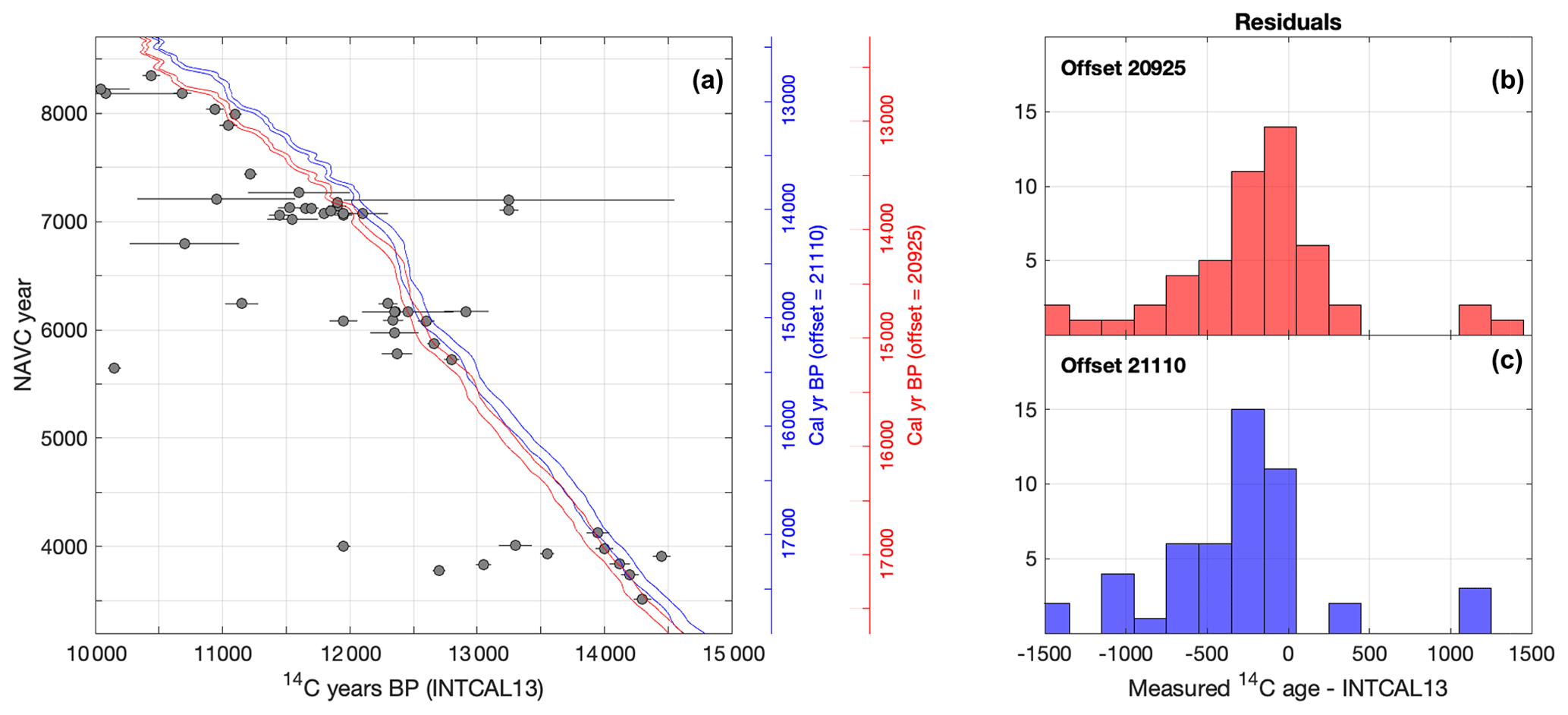
Figure 23(a) Alignment of radiocarbon ages of plant macrofossils in NAVC varves (Ridge et al., 2012; Thompson et al., 2017) with the INTCAL13 radiocarbon calibration curve for values of the NAVC–GICC05 yr BP offset estimated from 10Be flux matching (Figs. 18, 22) and the assumption that GICC05 years are equivalent to calendar years. The bands outlined in red and blue are the 68 % uncertainty bounds for the INTCAL13 calibration assuming offsets of 20 925 and 21 110, respectively. The histograms in (b) and (c) show residuals defined as the difference between the measured radiocarbon age of a sample from a particular varve year and the age predicted for that year by the INTCAL13 calibration and the selected offset.
On the other hand, applying the NAVC–GICC05 yr BP offset of 21 110 obtained from 10Be flux matching to the KF–GL records results in a poor alignment between INTCAL13 and the NAVC radiocarbon data set. Predicted 14C ages with this offset are nearly all older than observed, resulting in both the mode and the mean of the residuals being less than zero (Fig. 23) and requiring that essentially all 14C ages be spuriously young due to contamination. Adding the proposed ∼ 175-year undercount in the GICC05 timescale between ∼ 13 000 and ∼ 17 000 yr BP (Adolphi et al., 2018) worsens the agreement.
We conclude that (i) the apparent NAVC–ice core 10Be flux match at Newbury is consistent with the 14C data set, but (ii) the apparent match to the KF–GL record results in a value of the offset that is too old to be consistent with the 14C data.
4.2.5 Comparison of NAVC–GICC05 yr BP offsets inferred from 10Be flux matching with those inferred from correlation of varve and ice core climate records
In addition to calibrating the NAVC to calendar years using 14C ages, Ridge et al. (2012) and Thompson et al. (2017) proposed NAVC–GICC05 offsets based on correlation between abrupt climate changes in Greenland recorded in ice core δ18O records and ice-marginal events recorded by the NAVC. The premise of this approach is that rapid climate changes likely affected central Greenland and the margin of the LIS in the northeastern US similarly. Thus, cooling in Greenland should be associated with decreases in meltwater production, which are recorded by decreased varve thicknesses, and decreased ice margin retreat rates, or potentially stillstands or readvances, at the LIS margin. Warmings in Greenland should be associated with increases in meltwater production, varve thickness, and ice margin retreat rates. In this section, we evaluate whether these previously proposed correlations are consistent with the apparent NAVC–GICC05 matches based on comparing NAVC and ice core 10Be fallout discussed in the previous sections.
Events near 14 000 yr BP. For the period near 14 000 cal yr BP, Thompson et al. (2017) showed that the NAVC–cal yr BP offset of 20 825 years derived from fitting 14C data to INTCAL13 also yielded a close correlation between Greenland ice core climate records and events in the NAVC (Fig. 24a). This correlation associates a decrease in varve thickness near NAVC 6800 and increase near NAVC 6920 (Fig. 24) at Newbury with a rapid cooling and warming in Greenland at the boundaries of stadial GI-1d at 14 025 and 13 905 GICC05 yr BP, respectively (Lowe et al., 2008; Rasmussen et al., 2014), and places the beginning of the Littleton–Bethlehem Readvance, an ice margin readvance stratigraphically bracketed by NAVC varves 6836–6987, near the beginning of GI-1d.
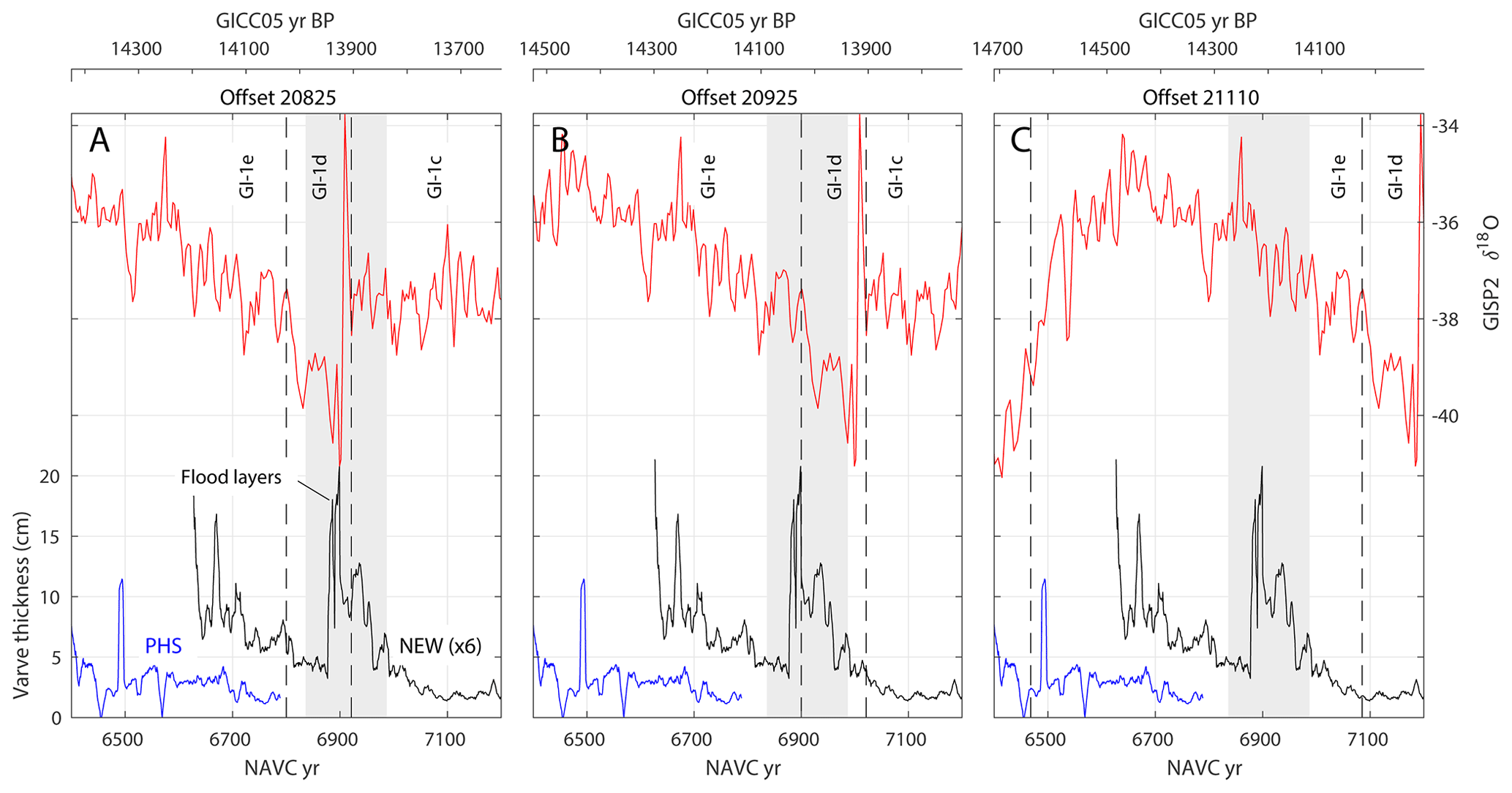
Figure 24Correlation between NAVC and GISP2 climate proxy records near 14 000 GICC05 yr BP. This duplicates Fig. 14 of Thompson et al. (2017), except that the x axis is reversed for consistency with the rest of the figures in this paper. Records at the bottom are 9-year running averages of varve thickness records from Newbury (NEWB) and Perry Hill Basin (PHS; see Ridge et al., 2012). The GISP2 δ18O record (Stuiver et al., 1995; Stuiver and Grootes, 2000) is a three-sample running average on the GICC05 chronology. The gray band shows the minimum duration of the Littleton–Bethlehem Readvance inferred from varves directly underlying and overlying the readvance till (see Thompson et al., 2017). Panel (a) uses the offset proposed as the best event correlation by Ridge et al. (2012) and Thompson et al. (2017), which is the same as the offset derived from fitting to INTCAL13 by Thompson et al. (2017). Panel (b) uses the offset that provides the best match between the 10Be flux at Newbury and the ice core stack (Fig. 22). Panel (c) uses the offset that provides the best match between the 10Be flux at KF–GL and the ice core stack (Fig. 18). Note that the anomalously thick varves near NAVC 6900 (highlighted in a) are related to a lake outburst flood and therefore have no climate significance (see Ridge et al., 2012). The Greenland climate event boundaries are from Rasmussen et al. (2014).
The NAVC–GICC05 offset of 20 925 years inferred from 10Be flux matching at Newbury (Fig. 22) implies that the Littleton–Bethlehem Readvance began in a precursory cold event prior to the start of GI-1d and ended at the GI-1d termination, which is stratigraphically permissible (Fig. 24b). On the other hand, this offset does not align appropriate varve thickness changes with the boundaries of GI-1d, so it is inconsistent with the hypothesis that cold events in Greenland should be associated with decreased meltwater production at the LIS margin. Therefore, accepting a NAVC–GICC05 yr BP offset of 20 925 years would require revising our understanding of the significance of the varve thickness changes at Newbury.
The NAVC–GICC05 yr BP offset of 21 110 inferred from 10Be flux matching at KF–GL (Fig. 18) does not yield any apparent correlation between ice core and NAVC climate proxy records in this time range, instead placing the Littleton–Bethlehem Readvance in a transitional phase of GI-1e (Fig. 24c) and yielding no obvious alternative correspondence between ice core climate and varve thickness records.
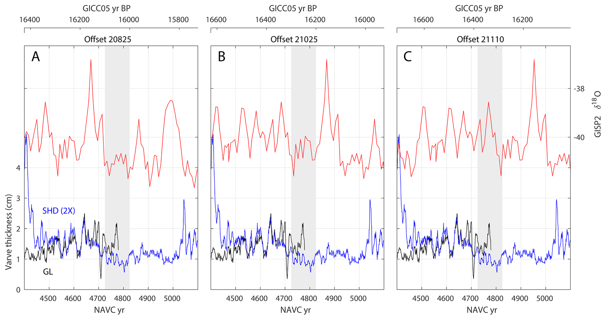
Figure 25Correlation between NAVC and GISP2 climate proxy records near 16 000 GICC05 yr BP. This duplicates Fig. 14a of Ridge et al. (2012), except that the x axis is reversed for consistency with the rest of the figures in this paper. The plot elements are the same as in Fig. 24. The gray band shows the Hatfield event, a period of slowed ice recession or a brief stillstand associated with thinner varves between NAVC ∼ 4725 and 4825.
Events near 16 000 yr BP. Ridge et al. (2012, their Fig. 14a) proposed that a NAVC–GICC05 yr BP offset of 20 825 years also aligned ice core climate and NAVC events at the time of the Hatfield event, an ice margin stillstand between NAVC 4725 and 4825. This event is associated with an abruptly bounded period of thinner varves at South Hadley (Fig. 25), and a 20 820 offset aligns this period with an unnamed minor cold phase in the ice core record (Fig. 25a). Although the NAVC–GICC05 yr BP offset of 21 110 instead aligns this event with a warm phase (Fig. 25b), a value of 21025, which is within the fairly broad range of acceptable matches at KF–GL, would align it with a different cold phase (Fig. 25c). It is also true, however, that the offset near 20 925 years inferred from 10Be flux matching at Newbury, with the proposed ∼ 150-year undercount in GICC05 in the 13.5–16 ka range (Adolphi et al., 2018), would result in an offset near the originally proposed value of 20820. Thus, event correlation around the Hatfield event is inconclusive as to whether the 10Be flux matches at either Newbury or KF–GL are valid.
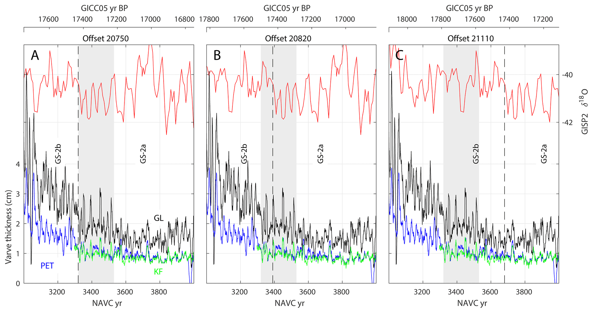
Figure 26Correlation between NAVC and GISP2 climate proxy records near 17 500 GICC05 yr BP. This duplicates Fig. 14b of Ridge et al. (2012), except that the x axis is reversed for consistency with the rest of the figures in this paper. The plot elements are the same as in Fig. 24. Varve thickness records shown are from Glastonbury (GL), Kelsey–Ferguson (KF), and South Windsor, CT (PET; see Ridge et al., 2012). The gray band shows the period of the Chicopee Readvance, which is associated with a period of thin varves at NAVC 3320–3530.
Events near 17 000 yr BP. Ridge et al. (2012, their Fig. 14a) proposed a NAVC–GICC05 yr BP offset of 20 750 years to align ice core and NAVC climate proxy records at the time of the Chicopee Readvance, which is associated with a period of thin varves near NAVC 3320–3530. They noted that this value of the offset aligns century-scale peaks in varve thickness with corresponding ice core δ18O variations during an unnamed cold phase (Fig. 26a). The value of 20 825 proposed as the best offset for event correlation around the Littleton–Bethlehem and Hatfield events fails to align these peaks and does not correlate the readvance with the cold phase (Fig. 26b). The NAVC–GICC05 yr BP offset of 21 110 years inferred from 10Be flux matching in this time range at KF–GL fails to align the Chicopee Readvance with any cold phase (Fig. 26c). However, if we accept the NAVC–GICC05 yr BP match at 20 925 from 10Be flux matching at Newbury and apply the estimate of Adolphi et al. (2018) wherein GICC05 is undercounted by ∼ 175 years between ∼ 13 500 and ∼ 17 000 BP, then a NAVC–GICC05 yr BP offset of 20 925 at Newbury implies a NAVC–GICC05 yr BP offset near 20 750 at the time of the Chicopee Readvance, which is the same as that proposed for event correlation by Ridge et al. (2012). Thus, the 10Be flux match at Newbury is consistent with event correlation around the Chicopee Readvance, but the 10Be flux match at KF–GL is not.
To summarize, the NAVC–GICC05 offset of 20 925 years suggested by correlation between NAVC and ice core 10Be records for the glacial section at Newbury may be consistent with previously proposed correlations between NAVC and ice core climate proxy records, but the NAVC–GICC05 offset near 21 110 suggested for the KF–GL section is not.
5.1 Systematics of Be deposition in varved glacial lake sediments
We found that the majority of 10Be in glacial and paraglacial varves in the NAVC is inherited and already adsorbed to sediment when supplied to the lake. This means that variation in the total 10Be flux to the lake predominantly reflects variations in the supply of inherited 10Be, which are mostly the result of grain size variations, and not variations in fallout 10Be. By using 9Be as a normalizing isotope, we were able to identify variations in the 10Be flux that are not explained by variations in the inherited Be supply to the lake and which we therefore attribute to variations in atmospheric 10Be fallout. In most cases, this yielded reconstructed 10Be fallout fluxes that were weakly correlated or uncorrelated with total Be fluxes, which supports the argument that this procedure is effective at separating environmental processes from fallout variations. This is an important element of this study: if we had not measured 9Be concentrations, it might be difficult or impossible to separate variations in inherited and fallout 10Be fluxes. Having quantified the relationship between grain size and Be concentrations in this study, however, it might be possible in future studies of the NAVC to extract variability in 10Be fallout without 9Be measurements by instead identifying variations in the total 10Be flux not explained by grain size, which would be similar to the approach of multivariate correlation with various sedimentological proxies applied in other studies (e.g., Czymzik et al., 2016). Regardless, using 9Be as a normalizing isotope appears simpler.
5.2 Variations in 10Be fallout flux
Our initial strategy in this study was to test the hypothesis that 10Be fallout variations are recorded in NAVC sediments by trying to identify the characteristic 11-year solar variability period in 10Be fallout variations. This strategy was not successful because of the high ratio of inherited 10Be to fallout 10Be in NAVC sediments. Expected fallout variability of 15 %–20 % around the mean associated with the 11-year solar cycle translates into variability in the total 10Be flux that has a similar magnitude as the measurement uncertainty. Thus, we were not able to distinguish short-period solar forcing of 10Be fallout variations, if present, from measurement noise.
On the other hand, in 1000-year varve sequences sampled with biennial resolution at two sites, we did observe centennial-scale variability in the reconstructed 10Be fallout flux resembling 10Be fallout variations observed in ice cores. This leads us to believe that 10Be concentrations in NAVC sediments do, in fact, record at least some prominent high-amplitude variations in 10Be fallout that can potentially be used to correlate NAVC and ice core records.
5.3 10Be systematics in glacial and paraglacial varve sequences
An unexpected result of this study is that glacial varves are likely better suited to reconstructing 10Be fallout than paraglacial varves. Initially, we supposed that paraglacial varves would be more likely to yield a record of 10Be fallout simply because they are typically an order of magnitude thinner than glacial varves, so 10Be fallout would be less diluted by higher sedimentation rates and associated larger inherited Be fluxes. This supposition was incorrect, and we found that variability in 10Be fallout was evident in glacial varve sequences but nearly entirely suppressed in paraglacial varves.
This result is most likely explained by the different roles of the watersheds that contribute to glacial and paraglacial lakes. In a paraglacial environment in which the lake is not receiving direct glacial meltwater, the lake watershed predominantly consists of a deglaciated landscape mantled by fresh glacial sediment. A significant fraction of 10Be fallout to the watershed is therefore adsorbed to sediment in developing soils, which limits the delivery of fallout 10Be to the lake and buffers variations in fallout rates.
In contrast, the contributing watershed of a proglacial lake in direct contact with the ice margin most likely includes large areas of the ablation zone of the ice sheet. Fallout 10Be cannot be stored on the ice in the ablation zone, so each year's fallout must be flushed into the lake by supraglacial or englacial discharge during the summer melt season. We hypothesize that this phenomenon can result in substantial focusing of fallout 10Be in glacial lake sediment and a minimal lag time between fallout variations and recording of those variations in glaciolacustrine sediment records. If true, this implies that varved glacial lake sediments, if deposited in a lake with a large supraglacial watershed, may be very effective recorders of atmospheric 10Be fallout. This hypothesis could easily be tested in modern proglacial lakes with large contributing areas on the ice surface, perhaps in west Greenland.
5.4 Correlation of the NAVC to ice core records by 10Be flux matching
We found values of the NAVC–GICC05 yr offset that resulted in acceptable correlations between reconstructed variations in 10Be fallout flux in NAVC sediments and an ice core 10Be flux stack for two varve sequences: a sequence at Newbury deposited near 14 000 yr BP and overlapping sequences at Kelsey–Ferguson (KF) and Glastonbury (GL) deposited ca. 16 000–17 000 yr BP. The NAVC–GICC05 yr BP offsets derived from these matches are not the same for both sections and also differ by 50–200 years from previously proposed values of the NAVC–calendar year offset inferred from radiocarbon dating of NAVC sediments and event matching between NAVC varve thickness records and Greenland ice core climate records.
Matching ice core 10Be records with 10Be fallout flux variations inferred from the older KF and GL varve sequences implies a NAVC–GICC05 yr BP offset in the range 20 965–21 165 years, with the best correlation at 21 110 years. However, the match between the two records mainly relies on aligning millennial-scale trends in the two records rather than distinct peaks associated with centennial-scale variations. As the KF–GL record is only 1000 years long, this could lead to spurious results. In addition, centennial-scale variations in the 10Be fallout flux in ice core records during this time period are relatively subtle. This match is not consistent with the NAVC–cal yr BP offset inferred from fitting NAVC 14C data to the INTCAL13 calibration curve, even when likely differences between the GICC05 ice core timescale and the true calendar year timescale are taken into account. Although offsets in the range implied by this match yield an acceptable correlation between ice core climate records and NAVC varve thickness records for events near NAVC 4800 and 16 000 GICC05 yr BP (Fig. 25), they are not consistent with the expected relationship between NAVC and ice core climate proxy records for younger or older periods (Figs. 24, 26). Overall, the apparent match between the KF–GL 10Be fallout flux and ice core 10Be does not appear consistent with most independent evidence and is unlikely to be valid.
Matching the 10Be fallout record from the glacial section at Newbury with ice core 10Be records, in contrast, relies on correlation of prominent large-magnitude, centennial-scale variations in both records and implies a NAVC–GICC05 offset in the range 20 900–20 940 (Fig. 22), with the best correlation at 20 925 years. This value of the offset is consistent with the 14C data set and, if the likely undercounting of ice core years in the GICC05 timescale between ∼ 13 000 and 17 000 yr BP is considered, also consistent with correlations between NAVC and Greenland ice core climate proxy records for periods surrounding the Hatfield event near NAVC 4800 and 16 000 GICC05 yr BP (Fig. 25) and the Chicopee Readvance near NAVC 3400 and 17 400 GICC05 yr BP (Fig. 26). This value of the offset yields an acceptable correlation between the stratigraphic boundaries of the Littleton–Bethlehem Readvance and the GI-1d stadial (Fig. 24) but does not clearly align the associated period of decreased varve thicknesses, which is interpreted to reflect decreased meltwater production during a cold period, with stadial boundaries. Thus, the 20 925-year NAVC–GICC05 yr BP offset inferred from 10Be fallout matching at Newbury is consistent with the majority of independent evidence and may be valid, but a reassessment of the climate significance of varve thickness variations associated with the Littleton–Bethlehem Readvance would be required to resolve all conflicts with independent data.
5.5 Weaknesses and strategy for improvement
The weakest part of our argument that the correlation between the 10Be fallout flux in NAVC sediments at Newbury and the ice core stack is valid is that the correlation is based on a short record comprising only 600 glacial varves that display two prominent peaks in reconstructed 10Be fallout flux. The ice core stack, on the other hand, includes three major fallout peaks between 14 000 and 15 000 GICC05 yr BP and a number of relatively high-amplitude secondary features. In addition, we only observed these 10Be fallout peaks at one section, so we cannot prove by replication between sections that they represent true fallout variations. Finally, the 25-year sampling resolution at Newbury is long relative to the size of the expected fallout peaks. For example, one of the most prominent apparent peaks is only represented by a single sample, and this effect alone could potentially explain much of the apparent ∼ 100-year difference between our proposed correlation based on the 10Be flux and that based on correlation of climate records in previous work. Another significant weakness derives from the property of our linear model for reconstructing the 10Be fallout flux that the apparent amplitude of reconstructed fallout variations displays a strong dependence on the value chosen for the inherited 10Be∕9Be ratio RS, so the amplitude of reconstructed fallout variations cannot be used as a point of comparison with ice core records. These weaknesses could in part be addressed by (i) higher-resolution sampling at the Newbury section to better resolve apparent fallout peaks and (ii) replication of the 10Be fallout record from additional varve sequences that overlap with Newbury in the range NAVC 6000–7000. Several overlapping sections exist, including the Perry Hill Basin site shown in Fig. 24, that could be used for this purpose. Higher-resolution 10Be measurements from older parts of the NAVC might be helpful in resolving whether or not the NAVC–ice core 10Be match at KF–GL is or is not valid, but they are less likely to be successful because 10Be fallout variability in the ice core stack between 15 000 and 18 000 GICC05 yr BP has a lower amplitude than that in the 13 000–15 000 GICC05 yr BP range. Overall, collecting higher-resolution 10Be data on replicate sections of glacial varves from the portion of the NAVC between approximately NAVC 5800 and the glacial–paraglacial transition near NAVC 7000 is likely the best strategy for resolving the remaining ambiguous results of this study.
All data are in the Supplement.
The supplement related to this article is available online at: https://doi.org/10.5194/gchron-3-1-2021-supplement.
All authors contributed equally. JCR had primary responsibility for correlation and sampling of varve sections, density measurements, and grain size measurements; BDD and PRB had primary responsibility for sample preparation; DHR had primary responsibility for AMS measurements; and GB had primary responsibility for data analysis and paper production.
Greg Balco is an editor of Geochronology.
We thank Kathyrn Lowe and Sarah Strand for help in the field and with grain size analysis, Sophie Greene for carrying out the 9Be measurements, Florian Adolphi for supplying ice core and stacked 10Be fluxes in an easily accessible form, and the staff of the AMS Laboratory at the Scottish Universities Environmental Research Centre (SUERC) for support with Be isotope ratio analyses. We particularly acknowledge the contributions of two anonymous reviewers in carefully reading the paper and providing constructive and helpful criticism. Greg Balco acknowledges financial support from the Ann and Gordon Getty Foundation, and all authors acknowledge financial support from the US National Science Foundation (NSF).
This research has been supported by the US NSF (grant nos. EAR-1103381, EAR-1103532, EAR-1103399, EAR-1103037, and EAR-0639830) and the Ann and Gordon Getty Foundation.
This paper was edited by Michael Dietze and reviewed by two anonymous referees.
Adolphi, F., Bronk Ramsey, C., Erhardt, T., Edwards, R. L., Cheng, H., Turney, C. S. M., Cooper, A., Svensson, A., Rasmussen, S. O., Fischer, H., and Muscheler, R.: Connecting the Greenland ice-core and U/Th timescales via cosmogenic radionuclides: testing the synchroneity of Dansgaard–Oeschger events, Clim. Past, 14, 1755–1781, https://doi.org/10.5194/cp-14-1755-2018, 2018. a, b, c, d, e, f, g, h, i, j, k, l, m, n, o, p, q
Aldahan, A., Possnert, G., Peck, J., King, J., and Colman, S.: Linking the 10Be continental record of Lake Baikal to marine and ice archives of the last 50 ka: Implication for the global dust-aerosol input, Geophys. Res. Lett., 26, 2885–2888, 1999. a
Andersen, K. K., Svensson, A., Johnsen, S. J., Rasmussen, S. O., Bigler, M., Röthlisberger, R., Ruth, U., Siggaard-Andersen, M.-L., Steffensen, J. P., Dahl-Jensen, D., Vinther, B. M., and Clausen, H. B.: The Greenland ice core chronology 2005, 15–42 ka. Part 1: constructing the time scale, Quaternary Sci. Rev., 25, 3246–3257, 2006. a, b
Antevs, E.: The Recession of the Last Ice Sheet in New England, American Geographical Society, New York, NY, USA, 1922. a
Antevs, E.: The Last Glaciation, with Special Reference to the Ice Sheet in Northeastern North America, American Geographical Society, New York, NY, USA, 1928. a
Balco, G., Stone, J. O., and Jennings, C.: Dating Plio-Pleistocene glacial sediments using the cosmic-ray-produced radionuclides 10Be and 26Al, Am. J. Sci., 305, 1–41, 2005. a
Bard, E., Raisbeck, G. M., Yiou, F., and Jouzel, J.: Solar modulation of cosmogenic nuclide production over the last millennium: comparison between 14C and 10Be records, Earth Planet. Sci. Lett., 150, 453–462, 1997. a
Beer, J., Blinov, A., Bonani, G., and Finkel, R.: Use of 10Be in polar ice to trace the 11-year cycle of solar activity, Nature, 347, 164–166, 1990. a
Belmaker, R., Lazar, B., Tepelyakov, N., Stein, M., and Beer, J.: 10Be in Lake Lisan sediments – A proxy for production or climate?, Earth Planet. Sc. Lett., 269, 448–457, 2008. a
Bierman, P., Brown, T., Caffee, M., Corbett, L., Fink, D., Freeman, S., Hidy, A.J., Rood, D., Wilcken, K., Woodruff, T., and Zimmerman, S.: Repeated preparation of CRONUS-N quartz standard for 10Be and 26Al at the University of Vermont and analysis at four different AMS laboratories, in: The 14th International Conference on Accelerator Mass Spectrometry, Ottawa, Canada, 14–18 August 2017. a, b, c
Binnie, S. A., Dewald, A., Heinze, S., Voronina, E., Hein, A., Wittmann, H., Von Blanckenburg, F., Hetzel, R., Christl, M., Schaller, M., Leanni, L., ASTER Team, Hippe, K., Vockenhuber, C., Ivy-Ochs, S., Maden, C., Fulop, R.-H., Fink, D., Wilcken, K. M., Fujioka, T., Fabel, D., Freeman, S. P. H. T., Xu, S., Fifield, L. K., Akcar, N., Spiegel, C., and Dunai, T. J.: Preliminary results of CoQtz-N: A quartz reference material for terrestrial in-situ cosmogenic 10Be and 26Al measurements, Nucl. Instrum. Meth. B, 456, 203–212, 2019. a
Boggs, S.: Principles of Sedimentology and Stratigraphy, Pearson Education, New Jersey, USA, 2014. a
Czymzik, M., Adolphi, F., Muscheler, R., Mekhaldi, F., Martin-Puertas, C., Aldahan, A., Possnert, G., and Brauer, A.: A varved lake sediment record of the 10Be solar activity proxy for the Lateglacial-Holocene transition, Quaternary Sci. Rev., 153, 31–39, 2016. a, b, c, d
Czymzik, M., Muscheler, R., Adolphi, F., Mekhaldi, F., Dräger, N., Ott, F., Słowinski, M., Błaszkiewicz, M., Aldahan, A., Possnert, G., and Brauer, A.: Synchronizing 10Be in two varved lake sediment records to IntCal13 14C during three grand solar minima, Clim. Past, 14, 687–696, https://doi.org/10.5194/cp-14-687-2018, 2018. a
Dettinger, M. D., Ghil, M., Strong, C. M., Weibel, W., and Yiou, P.: Software expedites singular-spectrum analysis of noisy time series, EOS, 76, 12–21, 1995. a, b
Feynman, J. and Fougere, P.: Eighty-eight year periodicity in solar-terrestrial phenomena confirmed, J. Geophys. Res.-Space, 89, 3023–3027, 1984. a
Finkel, R. and Nishiizumi, K.: Beryllium 10 concentrations in the Greenland Ice Sheet Project 2 ice core from 3–40 ka, J. Geophys. Res.-Oceans, 102, 26699–26706, 1997. a
Ghil, M., Allen, M., Dettinger, M., Ide, K., Kondrashov, D., Mann, M., Robertson, A. W., Saunders, A., Tian, Y., Varadi, F., and Yiou, P.: Advanced spectral methods for climatic time series, Rev. Geophys., 40, 1003, https://doi.org/10.1029/2000RG000092, 2002. a, b
Graly, J. A., Reusser, L. J., and Bierman, P. R.: Short and long-term delivery rates of meteoric 10Be to terrestrial soils, Earth Planet. Sc. Lett., 302, 329–336, 2011. a, b
Greene, E. S.: Comparing Meteoric 10Be, In Situ 10Be, and Native 9Be Across a Diverse Set of Watersheds, Master thesis, University of Vermont, Burlington, VT, USA, 110 pp., 2016. a, b
Hunt, A., Larsen, J., Bierman, P., and Petrucci, G.: Investigation of factors that affect the sensitivity of accelerator mass spectrometry for cosmogenic 10Be and 26Al isotope analysis, Anal. Chem., 80, 1656–1663, 2008. a
Jull, A. T., Scott, E. M., and Bierman, P.: The CRONUS-Earth inter-comparison for cosmogenic isotope analysis, Quat. Geochronol., 26, 3–10, 2015. a
Krumbein, W. C.: Size frequency distributions of sediments, J. Sediment. Res., 4, 65–77, 1934. a
Lal, D.: 10Be in polar ice: Data reflect changes in cosmic ray flux or polar meteorology, Geophys. Res. Lett., 14, 785–788, 1987. a
Lal, D. and Peters, B.: Cosmic ray produced radioactivity on the Earth, in: Kosmische Strahlung II/Cosmic Rays II, edited by: Sitte, K., Springer, 551–612, 1967. a, b
Lewis, D. W. and McConchie, D.: Analytical Sedimentology, Springer Science and Business Media, New Jersey, USA, 2012. a
Ljung, K., Björck, S., Muscheler, R., Beer, J., and Kubik, P. W.: Variable 10Be fluxes in lacustrine sediments from Tristan da Cunha, South Atlantic: a solar record?, Quaternary Sci. Rev., 26, 829–835, 2007. a, b, c
Lowe, J. J., Rasmussen, S. O., Björck, S., Hoek, W. Z., Steffensen, J. P., Walker, M. J., Yu, Z., Group, I., and INTIMATE Group: Synchronisation of palaeoenvironmental events in the North Atlantic region during the Last Termination: a revised protocol recommended by the INTIMATE group, Quaternary Sci. Rev., 27, 6–17, 2008. a, b
Mann, M., Beer, J., Steinhilber, F., and Christl, M.: 10Be in lacustrine sediments – A record of solar activity?, J. Atmos. Sol.-Terr. Phy., 80, 92–99, 2012. a, b
Muscheler, R., Joos, F., Beer, J., Müller, S. A., Vonmoos, M., and Snowball, I.: Solar activity during the last 1000 yr inferred from radionuclide records, Quaternary Sci. Rev., 26, 82–97, 2007. a
Nishiizumi, K., Imamura, M., Caffee, M. W., Southon, J. R., Finkel, R. C., and McAninch, J.: Absolute calibration of 10Be AMS standards, Nucl. Instrum. Meth. B, 258, 403–413, 2007. a
Pavich, M. J., Brown, L., Klein, J., and Middleton, R.: 10Be accumulation in a soil chronosequence, Earth Planet. Sc. Lett., 68, 198–204, 1984. a, b
Rasmussen, S. O., Seierstad, I. K., Andersen, K. K., Bigler, M., Dahl-Jensen, D., and Johnsen, S. J.: Synchronization of the NGRIP, GRIP, and GISP2 ice cores across MIS 2 and palaeoclimatic implications, Quaternary Sci. Rev., 27, 18–28, 2008. a
Rasmussen, S. O., Bigler, M., Blockley, S. P., Blunier, T., Buchardt, S. L., Clausen, H. B., Cvijanovic, I., Dahl-Jensen, D., Johnsen, S. J., Fischer, H., Gkinis, V., Guillevic, M., Hoek, W. Z., Lowe, J. J., Pedro, J. B., Popp, T., Seierstad, I. K., Steffensen, P., Svensson, A. M., Vallelonga, P., Vinther, B. M., Walker, M. J. C., Wheatley, J. J., and Winstrup, M.: A stratigraphic framework for abrupt climatic changes during the Last Glacial period based on three synchronized Greenland ice-core records: refining and extending the INTIMATE event stratigraphy, Quaternary Sci. Rev., 106, 14–28, 2014. a, b
Ridge, J.: The North American Glacial Varve Project, availabe at: http://geology.tufts.edu/varves (last access: May 2020), 2012. a, b
Ridge, J. C.: The Quaternary glaciation of western New England with correlations to surrounding areas, in: Developments in Quaternary Sciences, edited by: Ehlers, J. and Gibbard, P. L., Elsevier, 169–199, 2004. a
Ridge, J. C. and Toll, N. J.: Are late-glacial climate oscillations recorded in varves of the upper Connecticut Valley, northeastern United States?, GFF, 121, 187–193, 1999. a, b
Ridge, J. C., Balco, G., Bayless, R. L., Beck, C. C., Carter, L. B., Dean, J. L., Voytek, E. B., and Wei, J. H.: The new North American Varve Chronology: A precise record of southeastern Laurentide Ice Sheet deglaciation and climate, 18.2–12.5 kyr BP, and correlations with Greenland ice core records, Am. J. Sci., 312, 685–722, 2012. a, b, c, d, e, f, g, h, i, j, k, l, m, n, o, p, q, r, s, t, u, v, w, x, y, z, aa, ab, ac, ad, ae, af, ag, ah
Rittenour, T. M., Brigham-Grette, J., and Mann, M. E.: El Nino-like climate teleconnections in New England during the late Pleistocene, Science, 288, 1039–1042, 2000. a
Simon, Q., Thouveny, N., Bourlès, D. L., Valet, J.-P., Bassinot, F., Ménabréaz, L., Guillou, V., Choy, S., and Beaufort, L.: Authigenic 10Be/9Be ratio signatures of the cosmogenic nuclide production linked to geomagnetic dipole moment variation since the Brunhes/Matuyama boundary, J. Geophys. Res.-Sol. Ea., 121, 7716–7741, 2016. a
Steig, E. J., Morse, D. L., Waddington, E. D., and Polissar, P. J.: Using the sunspot cycle to date ice cores, Geophys. Res. Lett., 25, 163–166, 1998. a, b, c
Steinhilber, F., Abreu, J. A., Beer, J., Brunner, I., Christl, M., Fischer, H., Heikkilä, U., Kubik, P. W., Mann, M., McCracken, K. G., Miller, H., Miyahara, H., Oerter, H., and Wilhelms, F.: 9,400 years of cosmic radiation and solar activity from ice cores and tree rings, P. Natl. Acad. Sci. USA, 109, 5967–5971, 2012. a
Stone, J.: A rapid fusion method for separation of beryllium-10 from soils and silicates, Geochim. Cosmochim. Ac., 62, 555–561, 1998. a
Stuiver, M. and Grootes, P. M.: GISP2 oxygen isotope ratios, Quaternary Res., 53, 277–284, 2000. a
Stuiver, M., Grootes, P. M., and Braziunas, T. F.: The GISP2 δ18O climate record of the past 16,500 years and the role of the sun, ocean, and volcanoes, Quaternary Res., 44, 341–354, 1995. a
Thompson, W. B., Dorion, C. C., Ridge, J. C., Balco, G., Fowler, B. K., and Svendsen, K. M.: Deglaciation and late-glacial climate change in the White Mountains, New Hampshire, USA, Quaternary Res., 87, 96–120, 2017. a, b, c, d, e, f, g, h, i, j, k, l, m, n, o, p, q, r, s, t
Xu, S., Freeman, S. P., Rood, D. H., and Shanks, R. P.: Decadal 10Be, 26Al and 36Cl QA measurements on the SUERC 5 MV accelerator mass spectrometer, Nucl. Instrum. Meth. B, 361, 39–42, 2015. a
Yiou, F., Raisbeck, G., Baumgartner, S., Beer, J., Hammer, C., Johnsen, S., Jouzel, J., Kubik, P., Lestringuez, J., Stiévenard, M., Suter, M., and Yiou, P.: Beryllium 10 in the Greenland Ice Core Project ice core at Summit, Greenland, J. Geophys. Res.-Oceans, 102, 26783–26794, 1997. a