Towards an improvement of optically stimulated luminescence (OSL) age uncertainties: modelling OSL ages with systematic errors, stratigraphic constraints and radiocarbon ages using the R package BayLum

Statistical analysis has become increasingly important in optically stimulated luminescence (OSL) dating since it has become possible to measure signals at the single-grain scale. The accuracy of large chronological datasets can benefit from the inclusion, in chronological modelling, of stratigraphic constraints and shared systematic errors. Recently, a number of Bayesian models have been developed for OSL age calculation; the R package “BayLum” presented herein allows different models of this type to be implemented, particularly for samples in stratigraphic order which share systematic errors. We first show how to introduce stratigraphic constraints in BayLum; then, we focus on the construction, based on measurement uncertainties, of dose covariance matrices to account for systematic errors specific to OSL dating. The nature (systematic versus random) of errors affecting OSL ages is discussed, based – as an example – on the dose rate determination procedure at the IRAMAT-CRP2A laboratory (Bordeaux). The effects of the stratigraphic constraints and dose covariance matrices are illustrated on example datasets. In particular, the benefit of combining the modelling of systematic errors with independent ages, unaffected by these errors, is demonstrated. Finally, we discuss other common ways of estimating dose rates and how they may be taken into account in the covariance matrix by other potential users and laboratories. Test datasets are provided as a Supplement to the reader, together with an R markdown tutorial allowing the reproduction of all calculations and figures presented in this study.

1 Introduction

Optically stimulated luminescence (OSL, called optical dating in Huntley et al., 1985) allows the dating of the last exposure of quartz grains to sunlight. The single-aliquot regenerative (SAR) dose protocol consists of comparing the natural luminescence signal to laboratory-generated signals induced by artificial irradiation (Murray and Wintle, 2000; Wintle and Murray, 2006). The corresponding measurements, in particular at the single-grain scale, result in large datasets characterised by significant scatter, owing to a number of dispersion factors (see for example Thomsen et al., 2005). An OSL age is then obtained by dividing the equivalent dose (i.e. in the case of coarse quartz grains, the dose absorbed by the mineral) by the dose rate to which quartz grains were exposed since the last exposure to light.

Statistical analysis, in geochronology, generally aims to improve the precision, accuracy, and/or range of dating methods. In the case of OSL dating, calibration errors on the laboratory source dose rate for natural dose estimation, and geochemical standards for dose rate assessment, have so far resulted in age uncertainties (at 1σ or 68 % confidence) of, at best, ∼5 % (see for example Duller, 2008; Guérin et al., 2013).

Note that in what follows, the unit of analysis is a sediment sample; we assume that each sample corresponds to a deposition event, and thus to a single age (no post-depositional mixing is considered). The system of analysis is the laboratory in which the measurements are performed and includes both the apparatus and associated calibration standards. It should be emphasised here that field equipment is part of what we call the laboratory; this is important for the definition of what we call systematic errors. By definition, an error is the difference between the measured or observed value of a physical quantity and its true (but unknown) value. Thus, by systematic errors, we refer to random errors affecting equipment calibration: whereas each of these errors may be assigned a Gaussian probability density function with zero mean and a known variance (the square root of the variance being generally referred to as uncertainty), at the scale of the laboratory this error takes a fixed, unknown value that affects all measurements in the same direction. Of course, other sources of errors may exist (for example when using the infinite matrix assumption to calculate grain size attenuation factors; see for example Guérin et al., 2012b), but in this article, we consider only known, quantified sources of errors.

Over the past few years, several models for routine Bayesian analysis of SAR OSL and dose rate data were developed to better reflect, and take advantage of, the measurement procedures implemented to calculate OSL ages. Among those models, Combès et al. (2015) proposed one for calculating the central-dose values for well-bleached samples, leading to higher overall accuracy (see Guérin et al., 2015a) compared to the most commonly used model for OSL data analysis (the central-dose model: CDM, Galbraith et al., 1999; note that we changed the original terminology following Galbraith and Roberts, 2012). Combès and Philippe (2017) developed models capable of dealing with individual and systematic multiplicative errors for OSL age calculation including stratigraphic constraints (for general introductions on a statistical analysis of OSL data, but also the statistical models discussed hereafter and associated prior distributions, the reader is referred to Combès et al., 2015; Combès and Philippe, 2017, and references therein).

To implement the Bayesian models of Combès et al. (2015) and Combès and Philippe (2017) in practice, and provide easy access to the community, an R package (R Core Team, 2020) named “BayLum” (Christophe et al., 2020; version 0.2.0) has been developed and released on the Comprehensive R Archive Network (CRAN; see also Mercier et al., 2016, for a first implementation of the central-dose model developed by Combès et al., 2015). The first features of this BayLum package were presented by Philippe et al. (2019), and its performance, when one is confronted either with large dose values or with dose variability issues, was tested in laboratory-controlled experiments (Heydari and Guérin, 2018) and later applied to various case studies (Lahaye et al., 2018; Carter et al., 2019; Heydari et al., 2020, 2021; Chevrier et al., 2020).

The purpose of this paper is to focus on the treatment of stratigraphic constraints and systematic errors for chronological modelling using BayLum; i.e. it goes beyond than what was first demonstrated by Philippe et al. (2019). Together with the association of independent, more precise ages (¹⁴C in this work), such modelling is expected to reduce OSL age uncertainties. In the past, other approaches to model systematic and random, individual errors in the field of palaeodosimetric dating methods were proposed; in particular, Millard (2006a, b) developed a Bayesian approach quite close to that presented here, but which – among different other things (see Combès and Philippe, 2017, for a more detailed discussion) – is limited in its applicability.

Herein we present a Bayesian modelling case study. (1) We start with how data should be pre-treated prior to using the BayLum package; a simple example of chronological modelling (samples considered independent, i.e. without stratigraphic constraints and shared errors) is first presented, yielding an output from the BayLum package to serve as a reference for the following, more elaborate models. (2) In the next step, we detail how the user can integrate stratigraphic constraints and the effect on the chronological inference. It should be noted that we take here the stratigraphic information for granted, but we warn the user against treating such information lightly, as it bears great consequences on the age calculation (see discussions in Heydari et al., 2020, 2021). (3) Then, most importantly, we explain how to build a dose covariance matrix in practice to take into account systematic errors (for the definition of this matrix, the reader is referred to Combès and Philippe, 2017) and what effect it has on a series of ages. (4) For this purpose, we base our approach on dose rate measurements as performed by Guérin et al. (2015b) at the IRAMAT-CRP2A laboratory. The effect of integrating independent data such as radiocarbon ages, which usually do not share systematic errors affecting OSL data, is then illustrated. (5) Finally, we discuss different ways to measure dose rates and various assumptions that can be made regarding the nature (systematic or random) of additional sources of errors in OSL dating (see also Rhodes et al., 2003, for a similar discussion).

To help the reader, we provide in the Supplement an R markdown document with commented lines of code and example datasets, so that everything presented here may be reproduced.

2 Samples and methods

2.1 Case study

To illustrate how to model OSL ages, both in stratigraphic constraints and sharing systematic errors, using the R BayLum package, we use the data from two sediment samples (FER 1 and FER 3) already dated by quartz OSL (Guérin et al., 2015b). These samples were taken from the archaeological site of La Ferrassie (France) and prepared following standard chemical preparation procedures applied to luminescence-dating samples. While modelling with BayLum may be applied to both multi-grain and single-grain OSL datasets, in the following we only focus on single-grain data, as this is probably where the need for appropriate statistical models is most acute (the reliability of multi-grain OSL has been demonstrated when using a plain average (mean) for palaeodose estimation; see for example Murray and Olley, 2002; for theoretical justification, see Guérin et al., 2017). Single-grain OSL data were measured using an automated Risø TL/OSL reader (DA 20) fitted with a single-grain attachment (Duller et al., 1999; Bøtter-Jensen et al., 2000). A standard SAR protocol (Murray and Wintle, 2000, 2003) was used to measure single-grain equivalent doses, after checking its suitability for the samples under investigation. A comparison between quartz OSL and feldspar infrared stimulated luminescence (IRSL) signals for these two samples, as well as comparison with radiocarbon, showed that these samples were well-bleached at the time of deposition and unaffected by post-depositional mixing. As a result, the use of central-dose models is fully justified (it should be noted here that at the time of writing, BayLum does not yet include the Bayesian model of Christophe et al., 2018, allowing the analysis of poorly bleached samples).

2.2 Data pre-treatment

The Bayesian modelling implemented in BayLum requires information of different natures: (i) raw OSL data in the form of BIN/BINX file(s), (ii) list(s) of grains to be included in the modelling (based on pre-defined selection criteria, e.g. on recycling and/or recuperation ratios), (iii) file(s) indicating how the data should be processed (signal integration channels, reproducibility of the instrument(s), etc.), and (iv) both natural (in Gy ka⁻¹) and laboratory (in Gy s⁻¹) dose rates. Based on these data, the calculations are performed all at once using Markov chain–Monte Carlo (MCMC) computations; as a result, unlike in standard frequentist data processing, there is no succession of steps in data analysis (for example, individual equivalent dose estimates are not parameterised, unlike when the CDM is used). While Combès et al. (2015) argue that this results in a better statistical inference about the age (or palaeodose), it also comes with a downside: the user cannot visualise the data during the statistical analysis. In particular, the fact that the user must specify the list of grains to be included in the analysis implies that one should always pre-treat the samples in a standard way, by using for example “Analyst” (Duller, 2015) or the R “Luminescence” package (Kreutzer et al., 2012, 2020) to visually check the data but also to investigate the effect of various selection criteria on the datasets (see for example Thomsen et al., 2016, on the effect of applying various selection criteria with frequentist statistical models; see Heydari and Guérin, 2018, for a similar study in a Bayesian framework).

In other words, using BayLum for age calculation should not, and does not, prevent the user from a careful and critical examination of the measured OSL data. In particular, before running age calculations using the BayLum package, it is important that the user already has identified potential problems – e.g. saturation and/or dose rate variability (see Heydari and Guérin, 2018, for adapted modelling solutions).

3 First simple model and output

We first ran the function Generate_DataFile() for the OSL samples FER 1 and FER 3, with the same lists of grains as those used for age calculation by Guérin et al. (2015b): all grains with an uncertainty smaller than 20 % on the first test dose signal were selected. A large number of grains appeared to be in saturation for these samples (in Analyst, there is no intersection of the natural $L/T$ signal, or the sum of this sensitivity-corrected natural signal and its uncertainty, with the dose–response curve). As a result, following Thomsen et al. (2016), an additional selection criterion was added, based on the curvature parameter of the dose–response curves. All grains for which the D₀ value, obtained with Analyst as described by Guérin et al. (2015b), was smaller than 100 Gy were rejected from the analysis (note however that such a selection criterion may not be necessary when working with BayLum: Heydari and Guérin, 2018).

In practice, the data are contained in two folders named after the samples and provided in the Supplement. Each folder contains one BIN/BINX-file (i.e. OSL measurements; note that only a small fraction of the measured grains is included in the Supplement) and four CSV files:

• “DiscPos.csv” lists all selected grains.

• “Rule.csv” gives the rules for generating $L_x/T_x$ data (integration channels for both the natural or regenerated and test dose signals, uncertainty arising from the reproducibility of the OSL measurements, and number of SAR cycles to remove for curve fitting, if any – it may, for example, be desirable to remove recycled points and/or IR depletion points).

• “DoseSource.csv” gives the laboratory source dose rate and its variance.

• “DoseEnv.csv” gives the dose rate to which the sample was exposed during burial.

We ran the function AgeS_Computation() with a prior age interval limited to between 10 and 100 ka for each sample (so that the bounds are far from the age values obtained using the arithmetic mean of equivalent doses, namely 37±2 and 40±2 ka, respectively). The dose–response curves were fitted, as in Analyst in our previous study, with single saturating exponential functions passing through the origin. All uncertainties, affecting both environmental and laboratory dose rates, were included in the calculation, as is common practice in luminescence dating; however, the covariance of ages was not modelled here, so the results are equivalent to those one would obtain by running subsequent individual age calculations for each of the two samples.

To run the AgeS_Computation() function, the user must choose a model for the distribution of individual equivalent doses around the central dose; the different options are Cauchy, Gaussian or lognormal distribution (in the latter case, the central dose may be estimated either by the mean or the median of the distribution). A Cauchy distribution (sometimes also called Lorentz distribution) is a symmetric distribution which was chosen by Combès et al. (2015) because it has heavy tails; i.e. extreme values have a non-zero probability. Hence, the Cauchy distribution seemed to be well-suited for the analysis of widely dispersed datasets including outlier values such as single-grain D_e distributions.

Coming back to the samples from La Ferrassie, on top of saturation problems Guérin et al. (2015b) also identified dose rate variability as an important factor of dispersion in equivalent doses: the values of the CDM overdispersion parameter for the D_e distributions of the samples were equal to 29±3 % and 35±3 %, respectively. If we assume that this overdispersion arises from dose rate variability to single grains of quartz, Heydari and Guérin (2018) using laboratory-controlled experiments showed that the Cauchy distribution and the CDM should both lead to ∼5 %–10 % age underestimation, because both models are biased. Consequently, we did not use the Cauchy distribution model. Instead, we modelled the equivalent dose distribution by a lognormal distribution (one could also have chosen a Gaussian function) from which the mean (rather than the median) was used to estimate the central dose. Indeed, Guérin et al. (2017) formally demonstrated that the median of the lognormal distribution (as used in the CDM) is a biased estimator and leads to age underestimates when dose rates are dispersed.

Table 1 Summary of credible intervals for the ages (in ka) of samples FER 1 and FER 3 estimated in the different modelled scenarios.

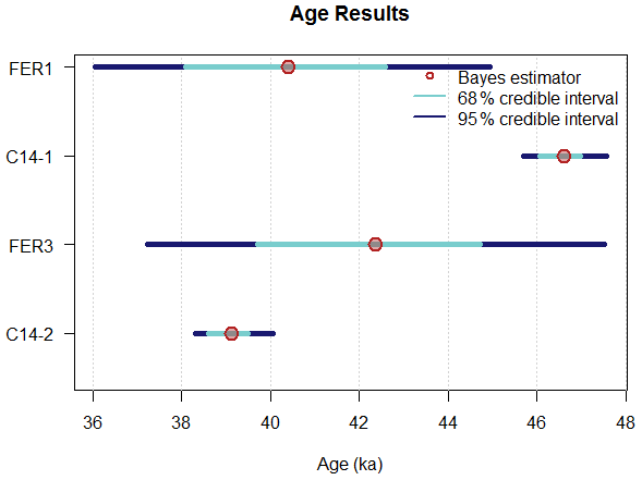
Figure 1 Age estimates for OSL samples FER 1 and FER 3. The red circles indicate the Bayes estimates of the age (i.e. the most likely values) for each sample; the cyan and blue bars represent the 68 % and 95 % credible intervals, respectively. For the two radiocarbon ages (C14-1 and C14-2), the reader is referred to Sect. 6.

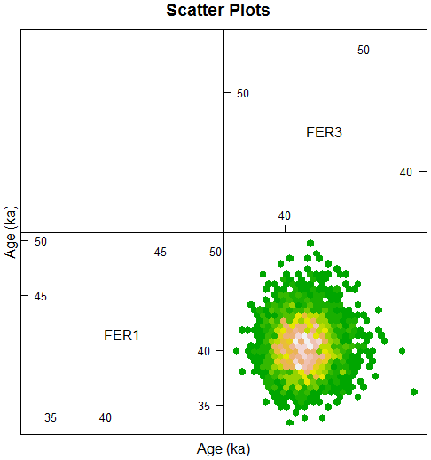
Figure 2 Bivariate scatter plot as hexagon plot presentation of a sample of observations from the joint posterior distribution of the two OSL ages considered independently (no stratigraphic constraints, no off-diagonal members in the covariance matrix). In such a plot, each point corresponds to one realisation of the ages of the two samples generated by the MCMC. Note that the reason for having this figure in the cell of an array is not visible here; it becomes useful when calculating ages for more than two samples, in which case for each pair of samples, a similar plot appears in the appropriate cell.

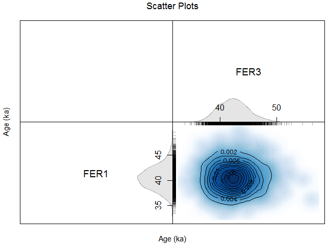
Figure 3 Probability densities for the OSL ages estimated jointly with the same model as that used to generate Fig. 2, based on kernel density estimates (KDEs), and marginal probability densities. The bell-shape and symmetry of the scatter plot indicate the absence of correlation between the two ages.

After 5000 iterations of three independent Markov chains, we observed good convergence, as seen in the markdown document provided in the Supplement (for a discussion of the convergence of the Markov chains, the reader is referred to Philippe et al., 2019). The upper limit of the 95 % confidence intervals for the Gelman and Rubin indexes of convergence (Gelman and Rubin, 1992) were all smaller than 1.05, also indicating satisfying convergence of the three independent Markov chains (here again, the reader is referred to Philippe et al., 2019, who suggested 1.05 as the maximum acceptable value). The obtained 95 % credible intervals (CIs) for the ages of samples FER 1 and FER 3 are [34.1; 43.3] ka and [36.6; 47.8] ka, respectively (Fig. 1; Table 1) and are consistent with the ages obtained by Guérin et al. (2015b) with a much simpler approach (unweighted arithmetic mean of equivalent doses). It should be emphasised here that the two 95 % CIs for ages overlap. Figure 2 shows a bivariate scatter plot of a sample of observations from the joint posterior distribution of the two ages, as generated by the Markov chains; in such a plot, each point corresponds to one realisation of the ages of the two samples investigated in the MCMC. Figure 3 shows the corresponding probability densities for the ages estimated jointly, based on kernel density estimates (KDEs), and the marginal probability densities. No correlation is observed on the joint probability density, which is symmetrical and bell-shaped. One can already compare the results obtained with this Bayesian model (lognormal-average) for sample FER 3 with the radiocarbon ages obtained independently for the same layer by Guérin et al. (2015b). The 95 % CI for the three ¹⁴C ages are bound by the interval [44.4; 47.3] ka, which means that the OSL and radiocarbon ages are in good agreement, which was not the case when calculating the ages with the CDM (38±2 ka; this OSL age corresponds to ∼15 % underestimation and is broadly consistent, within uncertainties, with theoretical predictions stated above). Thus, even without further modelling, the BayLum lognormal-average model seems to provide OSL ages in better agreement with radiocarbon.

4 Stratigraphic constraints

Samples FER 1 and 3 belong to two different stratigraphic layers: sample FER 1 (Layer 7) lies stratigraphically above sample FER 3 (Layer 5B), so we know that the age of the sample FER 1 must be less than that of the sample FER 3 (i.e. sample FER 1 is younger than sample FER 3; for detailed stratigraphic information on the site of La Ferrassie, which is of paramount importance in this section, the reader is referred to Guérin et al., 2015b). To encode this information, the function AgeS_Computation() takes as argument the object StratiConstraints, which is a matrix whose size depends on the number of analysed samples. First, the data in the DATA object (which is the output of the function Generate_DataFile()) must be ordered in stratigraphic order from top to bottom: thus, in our case the list of names used by the function Generate_DataFile()is FER 1, FER 3 (rather than FER 3, FER 1). Then, the stratigraphic matrix contains numbers equal to 0 or 1, indicating the applied bounds to the age of each sample. The matrix contains a number of rows equal to the number of samples plus one and a number of columns equal to the number of samples. The first row contains the value 1 in each column, which indicates that the younger age bound specified as prior information (10 ka in our example, cf. Sect. 3 above) when running the function AgeS_Computation() applies to all samples. Then, for all j in $\mathit{\{}\mathrm{2},\mathrm{\dots },\text{Nb\_Sample}+\mathrm{1}\mathit{\}}$ and all i in $\mathit{\{}j,\mathrm{\dots },\text{Nb\_Sample}\mathit{\}}$, StratiConstraints[j,i] =1 if the age of sample whose number ID is equal to j−1 is less than the age of sample whose number ID is equal to i. Otherwise, StratiConstraints[j,i] =0. In practice, in our case StratiConstraints [1,] $=(\mathrm{1},\mathrm{1})$, StratiConstraints [2,] $=(\mathrm{0},\mathrm{1})$ (which means that sample FER 1 is not younger than itself but is younger than sample FER 3) and StratiConstraints [3,] $=(\mathrm{0},\mathrm{0})$ (which means that sample FER 3 is neither younger than sample FER 1 nor than itself). Note that in the markdown document provided in the Supplement, the corresponding code lines have comments to make this description easier to follow.

Running the function AgeS_Computation() with this matrix of stratigraphic constraints only marginally affects the ages; in this case, the 95 % CIs become [34.3; 42.9] ka and [38.1; 48.5] for samples FER 1 and FER 3, respectively (Table 1). One can also look at the bivariate scatter plot of observations from the joint posterior distribution (Fig. 4): one can see that this scatter plot is truncated in the upper left-hand corner – illustrating the fact that the age of sample FER 1 can never be greater than that of sample FER 3 (see Fig. 2 for comparison). By contrast, the KDE estimate (Fig. 5) also shows a positive correlation but does not reveal the truncation (whereas the stratigraphic constraint imposes a null probability for all pairs of ages above the 1:1 line).

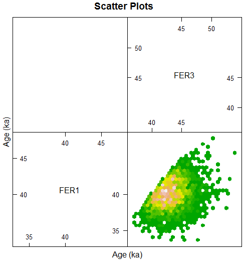
Figure 4 Bivariate scatter plot from the joint posterior distribution of the ages of samples FER 1 and FER 3 when a stratigraphic constraint is applied (sample FER 1 is younger than sample FER 3) but with no off-diagonal members in the covariance matrix. The truncation in the upper left-hand corner scatter plot indicates the effect of the stratigraphic constraint.

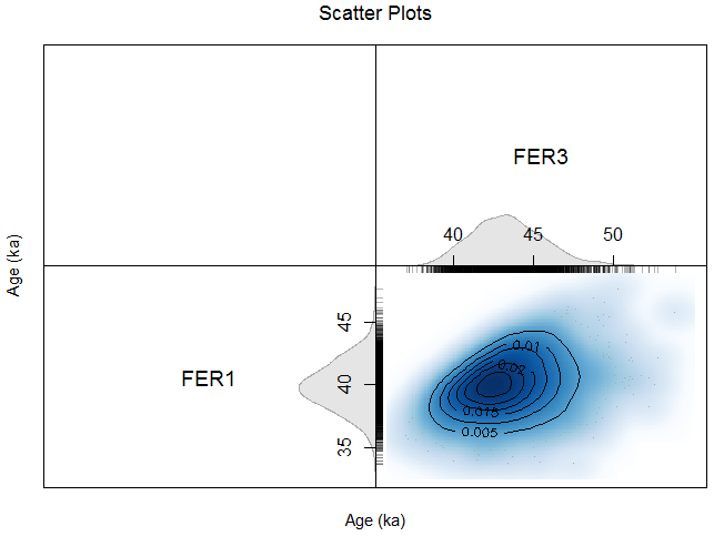
Figure 5 Probability densities for the OSL ages estimated jointly, using the same model as that implemented to generate Fig. 4 (stratigraphic constraint, no covariance matrix).

5 Dealing with multiple sources of errors through a covariance matrix

5.1 General considerations

In the previous calculations, all the variance is treated as random, whereas common, systematic errors affect all ages in the same direction, although to varying degrees (so systematic errors are unlikely to result in stratigraphic inversions). One of the main advantages of applying the models implemented in the BayLum package – contrary to other chronological modelling tools such as “OxCal” (Bronk Ramsey and Lee, 2013) or “Chronomodel” (Lanos and Philippe, 2018) – lies in the possibility to include the structure of uncertainties specific to OSL dating. For instance, a radiocarbon age is derived only from the ratio of ¹⁴C to ¹²C (on top of which comes the more complex problem of calibration), whereas an OSL age involves a large number of measurements, each with its uncertainty (Aitken, 1985, 1998). The OSL measurements required for the determination of the palaeodose are relatively standardised through the widespread use of the SAR protocol (Murray and Wintle, 2000; Wintle and Murray, 2006). Conversely, there are several approaches – each with its equipment and standards – to determine the various dose rate components. Given that these dose rates derive from different types of radiation (alpha, beta, gamma and cosmic radiation) and are of various origins (mainly from potassium and the uranium and thorium decay chains), there are many more contributions to the age uncertainty from the dose rate term than from the palaeodose term, even though the size of the uncertainty on dose rate is of the same order of magnitude as that on palaeodose – see for example Murray et al. (2015). As a result, there are almost as many ways of estimating systematic and random uncertainties as there are (combinations of) ways to determine dose rates; in any case, the notion of systematic error is only valid in a given context, which must always be made explicit. Combès and Philippe (2017) detailed the mathematical formulation of the dose covariance matrix, which links the ages of several samples measured using the same equipment and standards through common (systematic) errors (see also Philippe et al., 2019). Nevertheless, the equations provided in this article are somewhat difficult to translate in practice; here, we propose to outline how we implement a covariance matrix adapted to (one example of) the measurements leading to OSL age calculation at the IRAMAT-CRP2A laboratory (Bordeaux). We emphasise that what follows is not prescriptive; it should be viewed as an example of a model of uncertainties. For alternative ways of estimating systematic and random errors, for example, due to different dose rates measurements, the reader is referred to the discussion (Sect. 7.1).

Here, we consider the case of a series of n sediment samples taken from one unique site and all measured using the same equipment and standards. Let us consider the following relationship between palaeodoses, dose rates and ages (Combès and Philippe, 2017):

$$\begin{array}{}\text{(1)}& (D_{\mathrm{1}},\mathrm{\dots },D_n)\sim N\left(\left(A_{\mathrm{1}}{\dot{d}}_{\mathrm{1}},\mathrm{\dots },A_n{\dot{d}}_n\right),\mathrm{\Sigma }\right),\end{array}$$

where D_i is a random variable modelling the unknown palaeodose of sample i, N is the symbol for a Gaussian distribution, A_i is the unknown age estimate of sample i (that we are trying to determine), ${\dot{d}}_i$ is the total dose rate to which this sample was exposed since burial (${\dot{d}}_i$ is the observed dose rate, i.e. the result of the measurements) and Σ is the dose covariance matrix (for the full definition of the model, we refer the reader to Combès and Philippe, 2017). This covariance matrix verifies, for all (i,j),

$$\begin{array}{}\text{(2)}& {\mathrm{\Sigma }}_{i,j}=A_i{A}_j{\mathit{\theta }}_{i,j},\end{array}$$

where θ is the matrix that the user needs to specify to run the calculations with BayLum. It should be noted here that by default when running age calculations with BayLum, the off-diagonal elements are set to zero, i.e. the covariance in ages is not modelled.

Before entering the details specific to luminescence dating, let us consider a simple example of two measurements $y_{\mathrm{1}}={\mathit{\mu }}_{\mathrm{1}}+e_{\mathrm{1}}+f$ and $y_{\mathrm{2}}={\mathit{\mu }}_{\mathrm{2}}+e_{\mathrm{2}}+f$ where μ₁ and μ₂ are fixed measurands and e₁, e₂ and f are all independent random errors from distributions with mean zero. The covariance of y₁ and y₂ is the variance of f (so the off-diagonal elements of the matrix are equal to this variance). For each sample, the diagonal element of the corresponding covariance matrix is the sum of all the components of variance for that sample. The variety of physical quantities to measure and determine dose rate, and their relationship with the dose rate contributions, will now be discussed with this simple definition in mind.

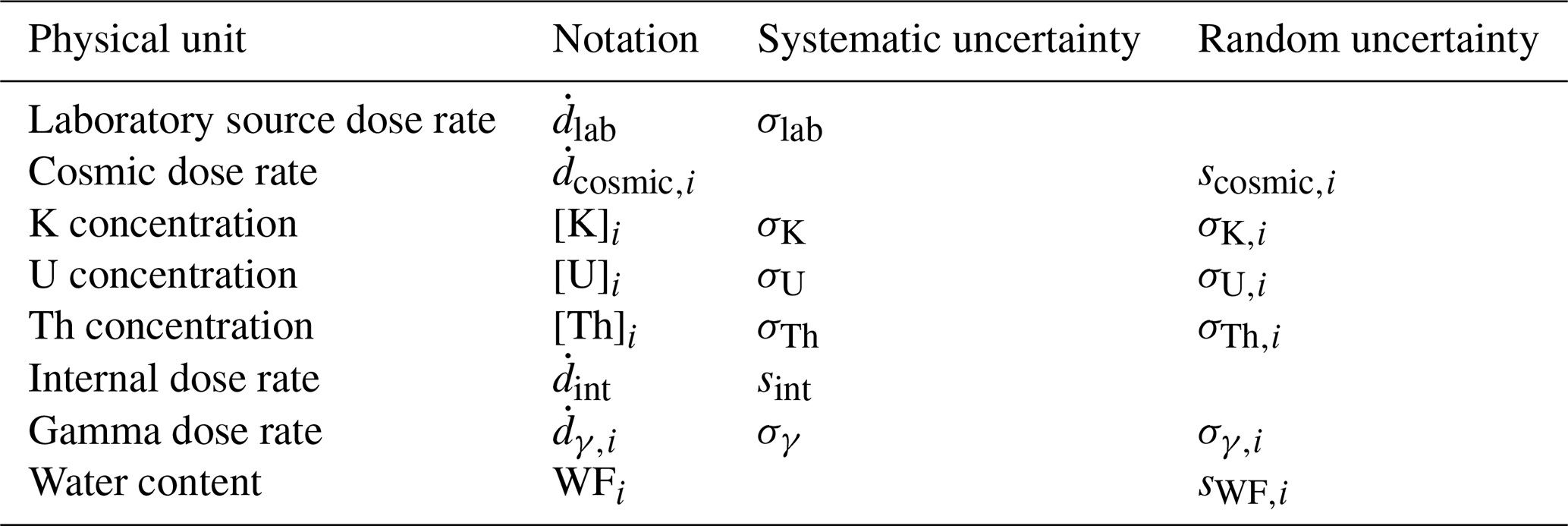
Table 2 List of physical units and associated uncertainties used in this work. The letter i in subscript indicates a sample specific value, its absence a common value shared between samples. The letter s indicates absolute uncertainties, while σ is used for relative uncertainties.

5.2 Implementation in practice

First, we detail the series of measurements carried out, and we introduce the corresponding notations for the estimates and associated uncertainties. Table 2 summarises all physical units and associated error standard deviations; as a general rule, we assume that all error terms are Gaussian variables with the expected value (mean) equal to zero and a fixed, known standard deviation (see for example Eq. 2 in Combès and Philippe, 2017). For clarity, in the following relative standard deviations are described by the letter σ, while absolute standard deviations are denoted by s; moreover, each standard deviation corresponding to random errors (i.e. when the error varies from sample to sample) is identified by the letter i in the subscript. The absence of this letter in the subscript indicates that the measurement error affects all samples.

5.2.1 Equivalent doses and OSL measurements

Equivalent doses are determined from OSL measurements performed on a luminescence reader equipped with a radioactive beta source, whose dose rate and associated relative standard deviation of the error, noted ${\dot{d}}_{\mathrm{lab}}$ and σ_lab, are known. There are several ways the latter term can be determined; in its simplest form, it includes the standard deviation of the error on the absolute dose absorbed by the standard reference material (in our case calibration quartz provided by DTU Nutech; see Hansen et al., 2015) and an error term due to replicate measurements of several aliquots of this calibration material. Using a large number of measurements repeated in time, as suggested by Hansen et al. (2015), may somewhat complicate the matter, but this goes beyond the scope of the present study.

In practice, regeneration doses are delivered by irradiating the aliquots for a given duration (in s). This duration is converted to absorbed energy dose (Gy) by multiplication with the source dose rate (Gy s⁻¹). Strictly speaking, the error on the source dose rate affects all regeneration doses, and so this error term should appear in the dose–luminescence relationship (right side of the directed acyclic graph shown in Fig. 7 of Combès and Philippe, 2017). However, it is common practice in luminescence dating to first calculate an equivalent dose in seconds of irradiation for each aliquot, then convert this to Gy and calculate an average (or determine another central parameter such as with the CDM), and only then consider σ_lab. This is what led (e.g., Jacobs et al., 2008) to the associated standard deviation being excluded from the total OSL age uncertainties, to test the assumption of a time gap between two series of ages. Here, for simplicity, we take the same route, and hence the relative error on the laboratory source dose rate becomes a relative, systematic error on the equivalent doses.

One may thus write that the error on the dose D_i arising from the calibration of the source follows a Gaussian distribution with mean 0 and variance $({\mathit{\sigma }}_{\mathrm{lab}}{A}_i{\dot{d}}_i{)}^{\mathrm{2}}$.

5.2.2 Dose rates

When it comes to the dose rate term, here we restrict ourselves to the case of coarse quartz grains measured after HF etching to remove the alpha dose rate component: the total natural dose rate is the sum of an internal dose rate, external beta and gamma dose rates, and cosmic dose rates.

Cosmic dose rates

We consider that cosmic dose rates are determined following Prescott and Hutton (1994) based on the burial depth of the dated samples, which may be different from the present-day thickness of the overburden. As a result, the error on cosmic dose rate estimates depends on the error estimation of this effective burial depth since the dated sediment was deposited. Because the relationship between cosmic dose rates and burial depths is not linear, and because the error on this burial depth may not be systematic (e.g. in cases where successive erosion and deposition events, of unknown duration, happened between the deposition of superimposed sedimentary layers – see Aitken, 1998, p. 65, for a discussion) even at the scale of a site, the error associated with cosmic dose rates cannot easily be treated as systematic. For $i=\mathit{\{}\mathrm{1},\mathrm{\dots },n\mathit{\}}$, ${\dot{d}}_{\mathrm{cosmic},i}$ and s_cosmic,i denote the estimate of the average cosmic dose rate to which sample i has been exposed and its associated standard deviation.

Beta dose rates

We consider the beta dose rates as determined from concentrations (or activities) of ⁴⁰K and in radioelements from the U and Th decay chains, converted to dose rates using specific conversion factors (e.g. Guérin et al., 2011). At the IRAMAT-CRP2A laboratory, these concentrations are usually determined with low-background, high-resolution gamma-ray spectrometry following Guibert and Schvoerer (1991). The simplest case is that of ⁴⁰K, since only one peak is used (at 1.461 MeV); the concentration in sample i, denoted [K]_i, is equal to the concentration in the standard multiplied by the ratio in count rates (the count rate observed for the investigated sample is divided by the count rate observed for a reference material). Thus, we consider in this paper that the standard deviation of the error on the ⁴⁰K concentration includes three components: the standard deviation of the error on the concentration in the standard sample, and the counting uncertainties both on the standard and on the measured sample. The counting uncertainties are calculated, assuming Poisson statistics. Of these three sources of errors, only one is treated as random – namely the counting uncertainty of the sample; the other two standard deviations (corresponding to the counting of the standard and to the error of the radioelement concentration in the standard) are quadratically summed and considered as a systematic source of error. One considers for sample i the beta dose rate from potassium ${\dot{d}}_{\mathit{\beta },\mathrm{K},i}$ – after correction for grain-size-dependent attenuation using the factors from Guérin et al. (2012b) and for moisture content following Nathan and Mauz (2008) (see the discussion section below regarding uncertainties on these correction factors). Neglecting uncertainties in the dose rate conversion factors, we call σ_K,i the relative random standard deviation of the error on the ⁴⁰K concentration; its systematic counterpart σ_K is common to all samples. It should be emphasised here that systematic errors on radioelement concentrations, although shared by all samples, will affect all ages in the same direction but not necessarily by the same amount (even in relative terms, contrary to the error on laboratory beta source calibration) because the relative contribution of beta dose rate from potassium to the total dose rate may vary from one sample to another. The beta dose rates from the U and Th series come from a number of radioelements in the corresponding chains; here, for simplicity we consider each series to be in secular equilibrium (this is generally the case for ²³²Th but may not be true for the U-series; see for example Guibert et al., 1994, 2009; Lahaye et al., 2012). Thus, for each sample, the concentrations in ²³⁸U and ²³²Th are converted to dose rate contributions denoted ${\dot{d}}_{\mathit{\beta },\mathrm{U},i}$ and ${\dot{d}}_{\mathit{\beta },\mathrm{Th},i}$. In contrast to the case of ⁴⁰K, the analysis of the high-resolution spectra for these radioactive chains is based on a number of primary gamma rays (whereas there is only one ray for K); more specifically, a weighted mean of the concentrations determined from each ray included in the analysis (after taking interference into account) is calculated to estimate the concentration of U and that of Th. As a result, the standard deviation of the error on the concentration in U (and that of Th) in the sample comes from two sources: the relative standard deviation on the concentration of the standard corresponds to a systematic error and is denoted σ_U for U (σ_Th for Th); conversely, the other relative standard deviations (arising from the counting of the standards and of the sample) are treated as random and quadratically summed to obtain σ_U,i (and σ_Th,i).

Internal dose rates

Unless the internal radioelement concentration is experimentally determined (in which case one needs to consider both systematic and random sources of error for each sample, as is done for beta dose rates), some have suggested using a fixed internal dose rate of 0.06±0.03 Gy ka⁻¹ (Vagn Mejdahl, personal communication to Andrew Murray, based on Mejdahl, 1987). In this case, we may assume that the dated quartz grains are all of the same origin and have the same internal radioelement concentration; as a result, we associate a systematic standard deviation s_int with the internal dose rate ${\dot{d}}_{\mathrm{int}}$.

Gamma dose rates

Gamma dose rates ${\dot{d}}_{\mathit{\gamma },i}$ may be determined, as beta dose rates, from K, U and Th concentrations in the sediment. In this case, the reader is referred to the corresponding section above. However, it is relatively frequent, in the case of heterogeneous configurations at the 10 cm scale, that gamma dose rates received by the samples do not correspond to the infinite matrix gamma dose rates of the samples (see for example large gamma dose rate variations at the interface between sediment and bedrock in a cave reported by Guérin et al., 2012a: Fig. 7). In such contexts, gamma dose rates may be determined by in situ measurements with Al₂O₃:C artificial dosimeters: these dosimeters are measured with green-light stimulation and their calibration is based on a block of homogeneous bricks located in the basement of IRAMAT-CRP2A (Richter et al., 2010; Kreutzer et al., 2018; note that we also discuss below – Sect. 7.1 – the use of portable spectrometers). Two sources of relative errors are taken into account: a random standard deviation (σ_γ,i) accounting for measurement uncertainties, and a shared calibration error including both standard deviations on (i) the true gamma dose rate in the block of bricks and on (ii) the measurement of the dosimeters irradiated inside the block for calibration of the source (σ_γ).

Water content

To account for the effect of water on dose rates, one commonly considers the following equation (Zimmerman, 1971; Aitken, 1985):

$$\begin{array}{}\text{(3)}& {\dot{d}}_{\mathit{\beta },i}={\displaystyle \frac{{\dot{d}}_{\mathit{\beta },i,\mathrm{dr}\mathit{\gamma }}}{\mathrm{1}+x_{\mathit{\beta }}{\text{WF}}_i}},\end{array}$$

where ${\dot{d}}_{\mathit{\beta },i,\mathrm{dr}\mathit{\gamma }}$ is the beta dose rate in the dry sediment, WF_i represents the effective mass fraction of water in the sediment during burial, and x_β is a water correction coefficient accounting for the fact that water absorbs more beta dose than typical sedimentary elements, due to lower atomic numbers (Nathan and Mauz, 2008). A similar equation applies to gamma dose rates, with a corresponding factor x_γ (see Guérin and Mercier, 2012). The determination of the water content in the sediment over time is a challenging task as it involves many different parameters, including past rainfall – see for example Nelson and Rittenour (2015) for a discussion on how to determine water contents depending on sediment grain size, hydrometric regimes, etc. One commonly employed solution is to measure the water content at the time of sampling and assume it to be representative of that in the past; measuring the water content at saturation may then be a solution to evaluate an upper limit to this value; and depending on the context one may also propose a lower limit to the water content. One then obtains a way of quantifying the standard deviation of the error on the water content, although necessarily imperfect. Neglecting uncertainties on the water correction factors (x_β and x_γ) and calling s_WF,i the absolute standard deviation of the mass fraction WF_i for sample i, one may write

$$\begin{array}{}\text{(4)}& s_{\mathit{\beta },{\mathrm{H}}_{\mathrm{2}}\mathrm{O},i}={\dot{d}}_{\mathit{\beta },i}{\displaystyle \frac{s_{\mathrm{WF},i}}{\mathrm{1}+x_{\mathit{\beta }}{\mathrm{WF}}_i}},\end{array}$$

where $s_{\mathit{\beta },{\mathrm{H}}_{\mathrm{2}}\mathrm{O},i}$ is the standard deviation of the beta dose rate for sample i due to the uncertainty on its water mass fraction.

Similarly, one may write

$$\begin{array}{}\text{(5)}& s_{\mathit{\gamma },{\mathrm{H}}_{\mathrm{2}}\mathrm{O},i}={\dot{d}}_{\mathit{\gamma },i}{\displaystyle \frac{s_{\mathrm{WF},i}}{\mathrm{1}+x_{\mathit{\gamma }}{\text{WF}}_i}},\end{array}$$

where $s_{\mathit{\gamma },{\mathrm{H}}_{\mathrm{2}}\mathrm{O},i}$ is the standard deviation of the gamma dose rate for sample i due to the uncertainty on its water mass fraction. As a result,

$$\begin{array}{}\text{(6)}& s_{\mathit{\gamma },{\mathrm{H}}_{\mathrm{2}}\mathrm{O},i}={\displaystyle \frac{{\dot{d}}_{\mathit{\gamma },i}}{{\dot{d}}_{\mathit{\beta },i}}}{\displaystyle \frac{\mathrm{1}+x_{\mathit{\beta }}{\text{WF}}_i}{\mathrm{1}+x_{\mathit{\gamma }}{\text{WF}}_i}}{s}_{\mathit{\beta },{\mathrm{H}}_{\mathrm{2}}\mathrm{O},i}.\end{array}$$

To simplify the following equations, which are meant to be those used in practice, we introduce the relative standard deviation of the beta dose rate due to water content errors (${\mathit{\sigma }}_{\mathit{\beta },{\mathrm{H}}_{\mathrm{2}}\mathrm{O},i}$) and a parameter called λ_i defined by

$$\begin{array}{}\text{(7)}& {\mathit{\lambda }}_i={\displaystyle \frac{\mathrm{1}+x_{\mathit{\beta }}{\text{WF}}_i}{\mathrm{1}+x_{\mathit{\gamma }}{\text{WF}}_i}}.\end{array}$$

Finally, it should be emphasised that uncertainty on water content may well correspond to errors which are neither really random nor really systematic; in our view different modelling choices may be put forward and implemented, depending on the particular sedimentological and pedological context.

The θ matrix

With these considerations in mind on errors and their nature, the corresponding θ matrix (Eq. 2) to model these uncertainties is a square matrix containing one line (and column) per sample. The diagonal elements correspond to the sum of a term arising from the error on the laboratory source dose rate (${\dot{d}}_i^{\mathrm{2}}{\mathit{\sigma }}_{\mathrm{lab}}^{\mathrm{2}}$) and the total dose rate variance for each sample, for each i:

$$\begin{array}{}\text{(8)}& \begin{array}{rl}{\mathit{\theta }}_{i,i}& ={\dot{d}}_i^{\mathrm{2}}{\mathit{\sigma }}_{\mathrm{lab}}^{\mathrm{2}}+s_{\mathrm{cosmic},i}^{\mathrm{2}}+{\dot{d}}_{\mathit{\beta },\mathrm{U},i}^{\mathrm{2}}\left({\mathit{\sigma }}_{\mathrm{U},i}^{\mathrm{2}}+{\mathit{\sigma }}_{\mathrm{U}}^{\mathrm{2}}\right)\\ & +{\dot{d}}_{\mathit{\beta },\mathrm{K},i}^{\mathrm{2}}\left({\mathit{\sigma }}_{\mathrm{K},i}^{\mathrm{2}}+{\mathit{\sigma }}_{\mathrm{K}}^{\mathrm{2}}\right)+{\dot{d}}_{\mathit{\beta },\mathrm{Th},i}^{\mathrm{2}}\left({\mathit{\sigma }}_{\mathrm{Th},i}^{\mathrm{2}}+{\mathit{\sigma }}_{\mathrm{Th}}^{\mathrm{2}}\right)\\ & +s_{\mathrm{int}}^{\mathrm{2}}+{\dot{d}}_{\mathit{\gamma },i}^{\mathrm{2}}\left({\mathit{\sigma }}_{\mathit{\gamma },i}^{\mathrm{2}}+{\mathit{\sigma }}_{\mathit{\gamma }}^{\mathrm{2}}\right)+\left({\dot{d}}_{\mathit{\beta },\mathrm{U},i}+{\dot{d}}_{\mathit{\beta },\mathrm{K},i}\right.\\ & {\left.+{\dot{d}}_{\mathit{\beta },\mathrm{Th},i}+{\mathit{\lambda }}_i{\dot{d}}_{\mathit{\gamma },i}\right)}^{\mathrm{2}}{\mathit{\sigma }}_{\mathit{\beta },{\mathrm{H}}_{\mathrm{2}}\mathrm{O},i}^{\mathrm{2}}.\end{array}\end{array}$$

This long list of variance terms may seem rather complicated. However, it corresponds to the total variance arising from the laboratory beta source calibration, the errors on cosmic dose rates, environmental beta dose rates, internal dose rates, gamma dose rates and finally the error arising from uncertainties in water content. In other words, we can also write

$$\begin{array}{}\text{(9)}& {\mathit{\theta }}_{i,i}={\dot{d}}_i^{\mathrm{2}}{\mathit{\sigma }}_{\mathrm{lab}}^{\mathrm{2}}+s_{{\dot{d}}_i}^{\mathrm{2}},\end{array}$$

where $s_{{\dot{d}}_i}^{\mathrm{2}}$ is the variance of the dose rate to which sample i was exposed to during burial (it is the square of the uncertainty appearing next to the dose rate value in every luminescence dating article; in our example, this term is the second one in the files DoseEnv.csv provided in Supplement).

Then, for i≠j,

$$\begin{array}{}\text{(10)}& \begin{array}{rl}{\mathit{\theta }}_{i,j}& ={\dot{d}}_{\mathit{\gamma },i}{\dot{d}}_{\mathit{\gamma },j}{\mathit{\sigma }}_{\mathit{\gamma }}^{\mathrm{2}}+{\dot{d}}_{\mathit{\beta },\mathrm{U},i}{\dot{d}}_{\mathit{\beta },\mathrm{U},j}{\mathit{\sigma }}_{\mathrm{U}}^{\mathrm{2}}+{\dot{d}}_{\mathit{\beta },\mathrm{K},i}{\dot{d}}_{\mathit{\beta },\mathrm{K},j}{\mathit{\sigma }}_{\mathrm{K}}^{\mathrm{2}}\\ & +{\dot{d}}_{\mathit{\beta },\mathrm{Th},i}{\dot{d}}_{\mathit{\beta },\mathrm{Th},j}{\mathit{\sigma }}_{\mathrm{Th}}^{\mathrm{2}}+s_{\mathrm{int}}^{\mathrm{2}}+{\dot{d}}_i{\dot{d}}_j{\mathit{\sigma }}_{\mathrm{lab}}^{\mathrm{2}},\end{array}\end{array}$$

which characterises the amount of correlation between the doses of samples i and j, multiplied by their ages. The θ matrix, like the dose covariance matrix Σ, is a symmetric matrix. The diagonal members correspond to individual variances, while the non-diagonal terms express the fact that systematic, shared errors link the measurements of the series of samples. As a result, running the functions AgeS_Computation() and Age_OSLC14() with a θ matrix in which all non-diagonal members are set to zero would be equivalent to running the same functions without the correlation matrix, or running the function Age_Computation() independently for each sample – in which case all sources of error are treated as random.

5.3 Examples

5.3.1 An illustrative, simplistic example without stratigraphic constraints

For illustration purposes, first, we did not apply stratigraphic constraints. We started with a simplistic θ matrix containing in the diagonal the real error variances (Eq. 9) as determined by Guérin et al. (2015b); the σ_lab value was equal to 0.02 (2 % relative standard deviation of the calibration of the laboratory beta source). The simplification comes from the off-diagonal members, for which in Eq. (10) we set all s and σ values to be equal to 0, except for the σ_lab value, set to 0.05. Obviously, this is not self-consistent, but it corresponds to (i) random and systematic errors of approximately the same magnitude (in practice, these two sources of errors are of the same order of magnitude – a few percentage points) and (ii) the simplest form of systematic errors. Indeed, in such a case, all ages are affected by the same relative amount in the same direction.

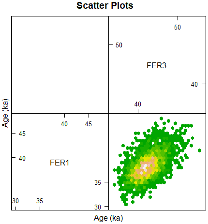
Figure 6 Bivariate scatter plot from the joint posterior distribution of the ages of samples FER 1 and FER 3 when a stratigraphic constraint is applied (sample FER 1 is younger than sample FER 3) and off-diagonal members of covariance matrix are used to model systematic errors (note that in this case, for illustrative purposes, we used a simplistic covariance matrix – see Sect. 5.3.1 for details). The truncation in the upper left-hand corner scatter plot indicates the effect of the stratigraphic constraint.

Figure 7 Probability densities for the OSL ages estimated jointly, using the same model as that implemented to generate Fig. 6 (stratigraphic constraint and off-diagonal members in the covariance matrix). The positive correlation in the joint posterior density reflects the effect of modelling the systematic errors with a covariance matrix (and, to some degree, of the stratigraphic constraint).

Here again, after 5000 iterations of three independent Markov chains, we observed good convergence. The obtained 95 % CIs are [33.9; 43.8] and [36.7; 48.1] ka for samples FER 1 and FER 3, respectively. Figure 6 shows bivariate scatter plots corresponding to the sampling of the Markov chains for the ages of samples FER 1 and FER 3 (which are calculated simultaneously), and Fig. 7 displays the KDE together with the marginal probability densities. This set of figures illustrates the reason for the generation of the two types of figures: the bivariate scatter plot is most appropriate for visualising the effect of stratigraphic constraints (Fig. 4 above), whereas probability density figures best illustrate the effect of modelling systematic errors. Indeed, as can be seen, there is a positive correlation between the ages of samples FER 1 and FER 3: the greater the age of sample FER 1, the greater the mean age of sample FER 3. In other words, if the age of sample FER 1 were underestimated, then in all likelihood, the age of sample FER 3 would also be underestimated. Furthermore, the length of the CI for the age of each sample is slightly larger than without modelling the covariance (cf. Table 1); i.e. modelling the covariances slightly increases the age uncertainties. However, the positive correlation of ages has other, direct consequences.

First, let us suppose that we have no knowledge of a stratigraphic link between the two investigated samples, and we wish to test the hypothesis that sample FER 1 is younger than sample FER 3. The credibility of such an assumption can be tested using the function MarginalProbability() of the “ArchaeoPhases” R package (Philippe and Vibet, 2020) devoted to the analysis of MCMC chains for chronological inference. Without using the covariance matrix, the credibility of this hypothesis is 0.83; with the simplistic θ matrix, the credibility becomes 0.94; in other words, modelling the age covariance reflects more faithfully the measurements and their uncertainties for such tests.

The second consequence concerns the duration of a hypothetical phase that would encompass the deposition of sample FER 1 and that of sample FER 3. Indeed, since the ages vary together in the MCMC, the duration of such a phase should be smaller when modelling the covariance than when all the variance in ages is treated as random. Indeed, we could verify this assertion using the function PhaseStatistics() of “ArchaeoPhases” (Philippe and Vibet, 2020): with the simplistic covariance matrix, the 95 % CI for the duration of this phase is [−1.4; 9.7] ka, whereas it is [−0.6; 7.6] ka when the ages are calculated using the simplistic θ matrix.

5.3.2 A real example, including stratigraphic constraints

In a real case, since the relative contributions of the different dose rate components vary from one sample to another, the correlation will be less pronounced. For more realistic calculations of the ages of samples FER 1 and FER 3, we took the same values as above for the diagonal terms of the θ matrix (Eq. 9); on the other hand, for the non-diagonal, covariance terms, we used the following values: σ_lab=0.02 (which corresponds to the experimentally determined calibration standard deviation, including the uncertainty of the dose delivered to calibration quartz; Hansen et al., 2015), σ_K=0.012, σ_U=0.007 , σ_Th=0.007 (for these values, which also include counting of the standards used, the reader is referred to Guibert et al., 2009; Guibert, 2002) and s_int=0.003 Gy ka⁻¹. In the Supplement we provide a calculation spreadsheet allowing the covariance matrix to be built, intended for adaptation to the user-specific needs.

At the site of La Ferrassie, the uncertainties associated with the gamma dose rate observations are more complex. Al₂O₃:C dosimeters were placed at the end of 25 cm long aluminium tubes and inserted horizontally in the stratigraphic section at the location of sediment sampling. In an ideal case, sediment should be uniform in a horizontal plane; however, for samples FER 1 and FER 3 only a rather thin layer of sediment remained against the cliff wall (the layers of the sample were not present at the site in any other location), which resulted in the dosimeters being inserted either in the karstic cliff (the limestone contains few radioelements compared to the sediments, as shown in Fig. 5 of Guérin et al., 2015b) or at the interface between the cliff and the sediment. As a result, we took for ${\dot{d}}_{\mathit{\gamma },i}$ the average between the gamma dose rates measured in situ (which underestimate the real gamma dose rate because the effect of the cliff is over-represented) and the gamma dose rates derived from the K, U and Th concentrations in the samples. The associated standard deviation, σ_γ,i, was calculated as the difference between these two extreme values divided by 4, so that the 95 % CI covers all possible values. As this standard deviation is much larger than the analytical uncertainties, we neglected the latter and considered σ_γ,i to characterise random sources of errors since each sample has a different environment and may be more or less far from the cliff.

The samples FER 1 and FER 3 are directly above and below, respectively, the Châtelperronian layer at the site (layer 6). Sample FER 2 from this layer being poorly bleached, it is at present impossible to model with BayLum. However, an alternative to estimate the age of FER 2 consists of supposing that it has a uniform prior probability density between the ages of samples FER 1 and FER 3:

$$\begin{array}{}\text{(11)}& P\left(A_{\mathrm{2}}\mathrm{|}\text{data}\right)\sim \int \int {\displaystyle \frac{I_{\left[A_{\mathrm{1}};A_{\mathrm{3}}\right]}}{A_{\mathrm{3}}-A_{\mathrm{1}}}}\mathit{\pi }\left(A_{\mathrm{1}},A_{\mathrm{3}}\mathrm{|}\text{data}\right)\mathrm{d}{A}_{\mathrm{1}}\mathrm{d}{A}_{\mathrm{3}},\end{array}$$

where A_i is the age of sample i, $I_{\left[A_{\mathrm{1}};A_{\mathrm{3}}\right]}$ is the indicator function between A₁ and A₃, and π(A₁,A₃|data) is the posterior joint density of A₁ and A₃ knowing the data (i.e. the density estimated with BayLum). Doing so (see the markdown file for the corresponding code lines), working from the output of BayLum one obtains a 95 % CI of [36; 46] ka, which can be compared with the confidence interval of [36; 48] ka obtained by Guérin et al. (2015b) with minimum age modelling.

6 Integration of independent chronological data (radiocarbon)

The BayLum package also offers the possibility to include radiocarbon ages in the chronological models (Philippe et al., 2019); more specifically, radiocarbon ages are calibrated within BayLum, using the function AgeC14_Computation() or Age_OSLC14() (in the latter case the function necessitates at least one OSL age calculation). Introducing covariance matrices to account for systematic errors on OSL data does not reduce the OSL age uncertainties; however, it becomes particularly useful to correct for estimation biases when more precise ages, unaffected by these systematic errors, are integrated into the models. To illustrate this, we decided to construct two models constraining the age of FER 3; for illustration purposes, in this section, we used the simplistic θ matrix described above in Sect. 5.3.1. In the first case, we constrained the age of this sample by imposing that a “young” radiocarbon age (young compared to the age of sample FER 3 considered alone) has an age greater than sample FER 3. In practice, we arbitrarily took a radiocarbon age of 38 000±400 BP, which corresponds to [37.6; 39.9] ka cal. BP (95 % CI using the IntCal20 curve, Reimer et al., 2020; the calibration was performed using BayLum; see Philippe et al., 2019). Naturally, the credible intervals (both 68 % and 95 %) for sample FER 3 are shifted towards younger age values (see the truncation of the scatter plot illustrated in Fig. 3). So are the credible intervals for sample FER 1, since the ages of the two OSL samples are close to each other even when considered independently of radiocarbon data (in other words, the radiocarbon age “pushes” the age of sample FER 3, which in turn “pushes” the age of sample FER 1). In practice, the 95 % CIs become [33.3; 41.2] ka and [36.9; 42.3] ka for samples FER 1 and FER 3, respectively. It can be noted here that in such a case the precision of the age of sample FER 3 is increased (i.e. the length of the CI is much smaller than without the constraining radiocarbon age). More interestingly, in the second case, we constrained the age of sample FER 3 by imposing that an “old” radiocarbon age (old compared to the age of sample FER 3 considered alone) has an age younger than sample FER 3. In practice we – again, arbitrarily – took a radiocarbon age equal to 44 000±400 BP, which corresponds to [45.4; 47.4] ka cal. BP (95 % CI). Here again, the effect on the age of sample FER 3 is straightforward: the credible intervals are shifted towards older ages (the 95 % CI for the age of sample FER 3 becomes [45.7; 51.2] ka). Perhaps less intuitive is the effect on the age of sample FER 1, which is not directly constrained by radiocarbon: because the ages of the three samples are estimated jointly, and because of the systematic errors on the OSL ages, the age of sample FER 1 is also shifted towards older ages: the corresponding 95 % CI becomes [36.7; 45.8] ka.

7 Discussion

7.1 Differing ways of estimating dose rates

Every laboratory uses its specific equipment and calibration standards; if similar equipment to that described above is used, then only the values of the different terms need be changed. This case is particularly relevant for equivalent dose measurements, and hence the term σ_lab associated with ${\dot{d}}_{\mathrm{lab}}$. Conversely, for dose rate determination, several other experimental devices and techniques are commonly used. If beta and/or gamma dose rates are determined based on the determination of concentration in K, U and Th, (by mass spectrometry, neutron activation, etc.), then the situation is similar to that described for beta dose rates above.

Counting techniques (alpha, beta and gamma in the case of the threshold technique: Løvborg and Kirkegaard, 1974) may also be used for beta and gamma dose rate estimation. In the case of beta counting, the conversion factor from count rate to dose rate depends on the emitting radioelement (Ankjærgaard and Murray, 2007; see also Cunningham et al., 2018). This dependency is a source of error that may not easily be characterised by a systematic error (so there is no contribution to the dose covariance matrix); indeed, this error on the conversion factor will vary from one site to another depending on the concentrations in K, U and Th (which are generally unknown if a counting technique is used), and even within one site from one sample to another (again by unknown amounts since the variability in K, U and Th is unknown).

The data acquired with field gamma spectrometers may be analysed in two ways: the “window” technique (see for example Aitken, 1985) corresponds to classical spectrometry analysis; in this case, the structure of uncertainties is the same as that for beta dose rates determined from high-resolution gamma spectrometry (Eq. 11). On the other hand, threshold techniques consist of taking advantage of proportionality between gamma dose rates and (i) the number of counts recorded per unit time above a threshold (Løvborg and Kirkegaard, 1974) or (ii) the energy deposited per unit time above a threshold (energy threshold: Guérin and Mercier, 2011; Miallier et al., 2009). In the former case, the conversion from count rate to dose rate depends on the emitting radioelement, so no systematic error term may be isolated. Conversely, in the latter case (energy threshold), this dependency is negligible (Guérin and Mercier, 2011). As a result, the error on the dose rate of the calibration standard may be considered as systematic and thus contribute one term in the non-diagonal elements of the covariance matrix. Difficulties in implementing the threshold technique may occur in low-dose-rate environments, because energy calibration may not be straightforward if the probe is not self-stabilised. In such cases, routines such as those implemented in the R package “gamma” (Lebrun et al., 2020) may be put to profit. Finally, ageing of the crystal may also result in time-dependent errors – the latter must be taken care of by regular calibration experiments.

7.2 Error terms neglected in this study

As mentioned earlier in the section devoted to dose rate uncertainties, there are many possibilities to quantify but also to consider errors in dose rate measurements; one could mention here the uncertainties on attenuation factors and water correction factors. However, both of these factors are dependent on the infinite matrix assumption: attenuation in grains implies that something other than the grains does not attenuate radiation (i.e. conservation of energy implies that if there is lower dose rate inside a quartz grain, there must be a higher dose rate somewhere else – see Guérin et al., 2012b); water correction factors are often calculated assuming a homogeneous mixture of water and other sedimentary components (Zimmerman, 1971; Aitken and Xie, 1990; note that the composition of the sediment also necessarily affects the ratios of electron stopping powers and photon interaction cross sections – see Nathan and Mauz, 2008, for a discussion). Limitations of this infinite matrix assumption, which is not met in sand samples at the scale of beta dose rates, have already been pointed out (Guérin and Mercier, 2012; Guérin et al., 2012a, b; Martin et al., 2015). Consequently, it seems that routine determination of a realistic standard deviation of the attenuation and water content correction parameters is not straightforward.

Dose rate conversion factors were assumed above to be known without error; however, estimation errors affect half-lives, emission probabilities, average emitted energies, etc. Liritzis et al. (2013) took these uncertainties into account to estimate standard deviations of the dose rate conversion factors (in practice, these standard deviations amount to ∼1 % for K dose rates, ∼2 % for U and ∼2 % for Th). These standard deviations could be included as sources of systematic errors when the contributions of K, U and Th are determined separately (note that when this is not the case, as when dosimeters are used for gamma dose rate estimation, or when beta counting is implemented for beta dose rate assessment, these sources of errors should be treated as random).

In this study, we worked with coarse-grain quartz extracts that had been etched with HF to remove the alpha-irradiated part of the grains. This being said, if alpha dose rates are taken into account, then the situation becomes similar to that of beta dose rates treated above; however, the sensitivity to alpha irradiation must then be taken into account. It is rather frequent in such a case to use published values from the literature (e.g. Tribolo et al., 2001; Mauz et al., 2006). Depending on the geological origin of the quartz (one or more sources), one may then assume either systematic or random errors in the alpha sensitivity.

7.3 Publication habits and re-analysis of previously published ages

Compared to other statistical models for OSL dating, the Bayesian models implemented in BayLum appear rather complicated, at least partly because modelling starts from the measured OSL data. By comparison, the input data to the CDM or the Average Dose Model (ADM: Guérin et al., 2017) are lists of equivalent doses and associated uncertainties, which means that OSL measurements have already been analysed to derive equivalent doses. Combès et al. (2015) argued that their complete model (implemented in BayLum), relating all the variables to one another, produces a more homogeneous and consistent inference compared to consecutive inferences (and indeed, when approaching saturation, i.e. when equivalent doses and associated uncertainties can hardly be parameterised, Heydari and Guérin (2018) demonstrated the advantage of BayLum models compared to parametric models such as the CDM and ADM). However, working with lists of equivalent doses and uncertainties – or even with estimates of central doses and associated uncertainties – taken as observations would make the Bayesian modelling proposed in BayLum and described in this paper more straightforward and transparent. Such an approach, called the “two-steps” model by Combès and Philippe (2017; see also Millard, 2006a, b, for earlier, similar models), would also offer the advantage of allowing re-analysis of already published data to derive more precise chronologies. However, for this purpose, the breakdown of all uncertainties and related standard deviations of errors is needed; nowadays, providing such key information for the modelling is not in the luminescence dating community's publication habits. That being said, with the growing number of meta-analyses of previously published data, and the availability of models such as BayLum to combine measurements with systematic errors, these habits might evolve in the future.

7.4 Notes of caution

As always when working with statistical models, one should first and foremost evaluate the measured data in light of the sampling context. We already mentioned the importance of grain selection (Sect. 2.2); but, perhaps more importantly, and especially since users of BayLum have to make modelling choices (e.g. regarding the dose–response curves fitted to OSL measurements or the distribution of individual equivalent doses around the central dose), it is crucial to carefully examine data and assess their quality before building potentially sophisticated models.

We would like to emphasise a few warnings regarding modelling samples in stratigraphic constraints, and the association of ages obtained by different methods. We would advise users, before combining for example radiocarbon and OSL ages, to first thoroughly examine the corresponding datasets independently: how were the data produced (with which experimental procedure)? Are the provided uncertainties reliable (or is there an unrecognised source of error that should be included in the evaluation of uncertainty)? Users are also encouraged to examine the consistency of results produced by each method, in light of the stratigraphy. In a second stage, before modelling of independent ages, we would recommend assessing the consistency of these datasets – do they (at least broadly) agree? If not, can a parsimonious explanation be found? For example, it is rather common, when performing Bayesian modelling with tools such as OxCal, to observe a large fraction of ages considered as outliers; such observations should urge users to examine their data again and come up with likely explanations (note that to date, no outlier model has been developed for the OSL ages in BayLum).

When it comes to imposing ordering constraints between ages as a result of stratigraphic observations, it is, of course, essential to leave no doubt about the validity of these stratigraphic constraints (the results of a model depend on the assumptions that are made, and the order in ages is a very strong constraint). Perhaps more importantly, even when stratigraphic constraints are valid, it is possible that applying them will not improve the statistical inference.

A simple example to illustrate this point is that of two superimposed, distinct layers (so that a stratigraphic order is clear) whose true ages are equal (or in practice, for which the age difference is negligible compared to the typical uncertainties of the implemented dating method). In such a case, modelling the ages with stratigraphic constraints is likely to result in a loss of accuracy (the age of the older layer will be overestimated, and that of the younger layer underestimated) compared to a model where no stratigraphic constraints are imposed. Future developments of the BayLum package might include the possibility to test different modelling scenarios by comparing the agreement between the observations and the posterior probability densities, for example using the Bayes information criterion (BIC).

8 Conclusion

New models for building chronologies based on OSL, with the possibility to incorporate radiocarbon, have been proposed in the literature (Combès et al., 2015; Combès and Philippe, 2017). These models have been demonstrated to improve the chronological inference based on OSL data and in particular, the accuracy of OSL ages (Guérin et al., 2015a; Heydari and Guérin, 2018). The R package BayLum was developed to implement these models; Lahaye et al. (2018), Carter et al. (2019) and Heydari et al. (2020, 2021) have used some of them to establish the chronologies of sedimentary sequences dated by OSL, resulting in generally more precise chronologies.

In this article, we have presented a case study on how to build simple models and observe output data, particularly through bivariate plots of age probability densities. Then, we have shown how to include stratigraphic constraints in the models; we have described how to fill the covariance matrices to account for systematic errors in OSL age estimation; and we have shown the effect of including independent age information in the models, namely radiocarbon ages. Different tools to visualise and further analyse the output of BayLum were demonstrated.

As a result, it is now possible to use various sources of information often available in practice when dating stratigraphic sequences. Age inferences based on OSL and independent data (e.g. radiocarbon) in stratigraphic constraints are expected to benefit in terms of accuracy, precision and robustness, through the application of such Bayesian models.