the Creative Commons Attribution 4.0 License.
the Creative Commons Attribution 4.0 License.
 | 21 Dec 2021
Deconvolution of fission-track length distributions and its application to dating and separating pre- and post-depositional components
Kirsten Hansen
To enable the separation of pre- and post-depositional components of the length distribution of (partially annealed) horizontal confined fission tracks, the length distribution is corrected by deconvolution. Probabilistic least-squares inversion corrects natural track length histograms for observational biases, considering the variance in data, modelization, and prior information. The corrected histogram is validated by its variance–covariance matrix. It is considered that horizontal track data can exist with or without measurements of angles to the c axis. In the latter case, 3D histograms are introduced as an alternative to histograms of c-axis-projected track lengths. Thermal history modelling of samples is not necessary for the calculation of track age distributions of corrected tracks. In an example, the age equations are applied to apatites with pre-depositional (inherited) tracks in order to extract the post-depositional track length histogram. Fission tracks generated before deposition in detrital apatite crystals are mixed with post-depositional tracks. This complicates the calculation of the post-sedimentary thermal history, as the grains have experienced different thermal histories prior to deposition. Thereafter, the grains share a common thermal history. Thus, the extracted post-depositional histogram without inherited tracks may be used for thermal history calculation.
- Article
(829 KB) - Full-text XML
- BibTeX
- EndNote


Fission of uranium-238 (U-238) in apatite, titanite, and zircon creates tracks in the crystal lattice. Track density is reduced as a function of temperature and time as tracks anneal and shorten due to atom diffusivity (Li et al., 2011; Fleischer et al., 1975; Afra et al., 2011). Ongoing track generation through time and simultaneous annealing is used to derive the thermal history of the sample. Bertagnolli et al. (1983) derived a differential equation describing the track length distribution within a mineral due to annealing through time. The surface density of tracks is also described. Forward-calculation examples are given by Bertagnolli et al. (1983). On this basis, Keil et al. (1987) developed an inversion procedure in which the temperature history is derived from either the length distribution of tracks within the crystal or from the length distribution of projected tracks intersecting the surface. The calculation procedure is direct and without the use of a Monte Carlo-type optimization. The time of track generation can be derived from the observed track length distribution independent of any annealing model (Keil et al., 1987):
where λ0 is the present track normalized length, ε is the fission-track production rate, and n(λ) is the measured number of fission tracks of length λ produced per volume. Equation (1) is understood as follows: the annealing properties of the mineral affect the final apparent age as well as the expected age of the oldest randomly oriented unetched track. However, the expected age of this track can be determined by counting the number of all tracks in a volume and dividing this by the track generation rate. In the simplified case of no spread of track lengths, the expected age of any given track is calculated by counting the number of shorter tracks plus one. This age is determined without the use of an annealing model. The unetched tracks are not routinely measured; etched confined horizontal tracks are measured instead. This paper explains how they can be used along with the surface track density to separate pre- and post-depositional components.
The temperature history is derived from the distribution of projected tracks along with an annealing model. Keil et al. (1987) showed, using a synthetic example for projected tracks, that the thermal history can be calculated numerically stepwise backward in time starting with the present temperature. The large uncertainties in the projection of tracks mean that the approach by Keil et al. (1987) is dubious. The selection of horizontal confined tracks is recommended instead (Laslett et al., 1984) – that is, “tracks identified by the constancy of focus over their entire length and strong reflection in incident illumination” (Gleadow et al., 1986b, 2019). The model by Keil et al. (1987) does not include blurring of track length histograms caused by the initial distribution of fission fragment energy (Jungerman and Wright, 1949), annealing and etching anisotropy, mineral composition, the uncertainty of measurement (Ketcham, 2003), and track selection biases (Jensen et al., 1992). Proportionality of the number of tracks in a track length histogram column and time assumed by Keil et al. (1987) is disturbed by the blurring. Jensen et al. (1992, 1993) extended Eq. (1) to confined horizontal tracks instead of projected tracks. Donelick (1988) introduced a fission-track inversion procedure based on principles like that of Jensen et al. (1992) and the present paper.
Three major biases appear to be important when deriving the equation for track age:
-
the surface track density bias, reflecting the likelihood that a track is exposed to etching on the surface. Here, an exponential approximation of surface track density versus mean track length for induced tracks annealed in the laboratory is used (Green, 1988).
-
the track length bias, reflecting the likelihood that a track is exposed to etching through fractures and tracks cutting the etched surface. Here, this is assumed to be proportional to the track length.
-
the selection bias, reflecting the likelihood that an etched track is accepted as horizontal. Here, we assume that tracks within a given angle from the horizontal are counted.
The alternative that all tracks in focus are accepted is discussed in Appendix D. Besides biases, there are a range of effects contributing to large observational deviations of track lengths, as has been documented in inter-laboratory comparisons (Ketcham et al., 2009). The effects are caused by (a) fluid filling track tips, (b) poorly chosen track tips, and (c) analyst inexperience. Variation in the number of tracks in a given length interval is dependent on the spontaneous character of fission. The disordering of the unique relationship between track length and time caused by various biases and variances is essentially restored by deconvolution of natural track length histograms (Jensen et al., 1992). Deconvolution is performed by mathematically simulated annealing (Kirkpatrick et al., 1983) and with the use of filters based on annealing of induced tracks in the laboratory. Jensen et al. (1992, 1993) and Jensen and Hansen (2018) used the fact that the corrected track ages can be derived separately from the thermal history, as shown by Keil et al. (1987). The columns of the deconvolved track length histogram are then converted to equivalent time intervals. The track ages are obtained by backward cumulation from long tracks toward short tracks. We do not assign an age to the bins of observed fission-track length histograms. Ages are assigned to the bins of the deconvolved (corrected) track length histograms which can then be used to age date thermal events. The procedure of deconvolution described in Jensen et al. (1992) is for measurements where the c-axis angle is not measured. When they are available, it is the practice to project the tracks on the crystal c axis following the procedure described by Donelick et al. (1999). As an alternative, the inversion method presented here uses 3D histograms. Age–length relations for corrected tracks are given explicitly in contrast to the indirectly embedded relations in the computer programs by Green et al. (1989), Lutz and Omar (1991), Ketcham (2005), and Gallagher (2012). Our age calculations are performed without sample temperature history modelling. The inversion procedure presented here is based on least-squares probabilistic inverse theory (Tarantola, 2005). The method is computationally fast.
Before entering the mathematics of age calculation, a recipe for age dating of an uplift event is given, including temperature calculation. First, an idealized model is considered with tracks generated continuously (not spontaneously), no length spreading during annealing, no etching, and no errors of measurements:
-
Construct a track length density histogram (numbers/volume) of the randomly oriented unetched tracks.
-
Convert the track length histogram into a histogram of time intervals by dividing the number of tracks in each column by the rate of track generation. Each column of this histogram represents the time it takes to generate the tracks belonging to the column.
-
Cumulate the time intervals from the youngest (longest tracks) to the oldest (shortest tracks) to obtain a histogram of track ages.
-
If the uplift is sufficiently pronounced, a statistically significant break is visible in the age histogram. The event is hereby “age-dated”.
-
The age of the event can be used to extract the pre-event track histogram from the left part (shortest tracks) of the cumulated ages and the post-event histogram from the right part (longest tracks). Up until this point, there has been no need for a track annealing model.
-
The post-event temperature history can now be calculated separately, which is useful if the pre-event tracks are of mixed origins. The temperature is calculated for each column of the time interval histogram, as explained in Jensen et al. (1992).
In practice, however, confined horizontal etched track length histograms are used together with the surface track density, for age dating and calculation of the history of temperature. Tracks are produced spontaneously, their lengths are spread during annealing, observations are biased, and measurements are uncertain. The recipe can then be written as follows:
-
Construct a track length histogram of the observed confined horizontal etched tracks.
-
Remove the spreading of track lengths by deconvolution (deblurring) of the observed histogram.
-
Use the deconvolved histogram for age dating and calculation of the history of temperature following the recipe from point 2 for the idealized tracks.
The recipes are based on the development by Bertagnolli et al. (1983), Keil et al. (1987), and Jensen et al. (1992). The reader can also refer to Donelick (1988) for a similar development. The procedure for calculating the temperature history based on the deconvolved track length histogram was presented by Jensen et al. (1992). At that time, deconvolution was performed by trial and error. Mathematically simulated annealing was later applied instead (Jensen and Hansen, 2018). Age dating and identification of inherited tracks using Tarantola inversion are presented in the next sections. The calculations are direct, and there is no use of Monte Carlo simulations. Readers unfamiliar with the technique of deconvolution may benefit from reading Appendix A before entering the Tarantola inversion technique.
Consider a mineral such as apatite and a time interval Δti in which randomly oriented fission tracks are generated with the initial track length Lo. The number of tracks per unit volume generated in the time interval is proportional to the fission decay frequency λf, the U-238 concentration c, and the length of the time interval Δti:
Here, N is the number of time intervals. The exponential decay of the U-238 nuclei is initially ignored. A track is generated for each fission; therefore, ni is also the number of originally randomly oriented tracks per unit volume. The track length histogram of the randomly oriented tracks per unit volume generated in a single time interval Δti is initially
Here, vectors are bold, the transpose T transforms rows into columns, and M is the number of track length bins. The tracks are gradually annealed from the initial length by temperature and time, leading to shorter tracks with the mean track length Li (Fig. 1). The tracks generated in the time interval Δti are distributed into various track length columns following partial annealing. At present, after partial annealing, the track length histogram is
For the tracks that are not annealed below the detection limit, the number of tracks per unit volume νi (not bold) is equal to the number of fissions in the time interval – that is,
The surface track density is initially , whereas for the present, it is σi (Fig. 1).
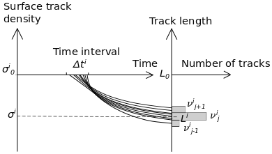
Figure 1In the time interval Δti, several tracks are spontaneously generated with the initial mean track length L0 and surface density . During anisotropic annealing over time, the initial length is reduced along the curved path and spread around the present mean length Li. Tracks from neighbouring time intervals are similarly spread and, consequently, mixed with tracks from the time interval Δti.
A fraction of the randomly oriented tracks νi cut other tracks connected to the surface, providing paths for etchants and making the tracks observable under a light microscope. The near-horizontal tracks are selected for length measurements. The track length histogram of the observed near-horizontal tracks generated in the time interval Δti is
Here, hi is expected to be linearly dependent on the randomly orientated unexposed tracks νi; thus, the histogram hi is derived by multiplying the histogram νi by a set of constants :
where K is a proportionality constant. Equation (7) relates the partly annealed randomly oriented unetched tracks to the observed horizontal tracks. The jth elements of hi is
The number of observable tracks generated in the time interval Δti is
Horizontal confined tracks of large area (the product of etched length and width) are likely to be etched. This means that the proportionality constants are as follows:
where is the track length of the partially annealed track. The relation between the randomly oriented tracks and the number of observable tracks is then
Equations (8) and (10) lead to
Summation on both sides of the equation leads to
which means that
It is expected that the shape and mean track length of the histogram hi of observable tracks with an origin in the time interval Δti can be reproduced in a laboratory annealing experiment:
Here, ![]() i is a proportionality constant, and gi is a track length distribution histogram derived from annealing in the laboratory, or an interpolation thereof:
i is a proportionality constant, and gi is a track length distribution histogram derived from annealing in the laboratory, or an interpolation thereof:
gi and hi have an identical number of tracks:
This is due to the fact that gi is normalized for all i:
The natural observed histogram is the sum over all the histograms hi, each of which is linked to time interval i:
and with Eq. (15),
Therefore, a natural fission-track histogram d can be approximated by a weighted sum of interpolated laboratory track length histograms (Figs. 2 and B1 in Appendix B).
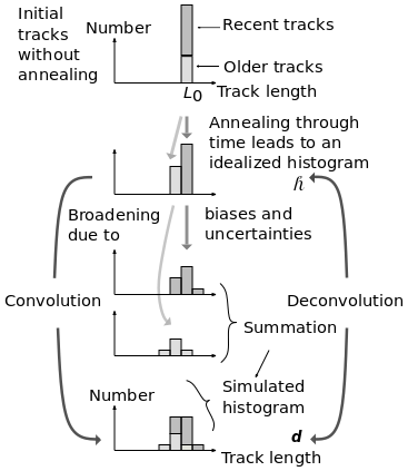
Figure 2All randomly oriented tracks start with the length L0 and are then annealed by time and temperature. At present, the track length histogram is ![]() , an idealized histogram without track length broadening effects. The most recent tracks appear in the right column of
, an idealized histogram without track length broadening effects. The most recent tracks appear in the right column of ![]() . This histogram is broadened by convolution to mimic the histogram d, resembling a measured histogram. The broadening is caused by the initial length range, biases, and uncertainties. The convolution itself may be regarded as a summation of the broadening of separate columns of
. This histogram is broadened by convolution to mimic the histogram d, resembling a measured histogram. The broadening is caused by the initial length range, biases, and uncertainties. The convolution itself may be regarded as a summation of the broadening of separate columns of ![]() . Deconvolution removes the broadening of d.
. Deconvolution removes the broadening of d.
gi is a filter transforming the weights ![]() i into the natural histogram d:
i into the natural histogram d:
or
Each column of the matrix G is a filter with increasing mean track length from column 1 to N. Solving Eq. (21) for ![]() (the model) is named deconvolution. Predictions using this equation are assumed to be error-free. Instead, the Bayesian framework (Bardsley, 2018) is used to include the probability density for (1) the observations dobs, (2) prior information
(the model) is named deconvolution. Predictions using this equation are assumed to be error-free. Instead, the Bayesian framework (Bardsley, 2018) is used to include the probability density for (1) the observations dobs, (2) prior information ![]() prior for the solution, and (3) the solution
prior for the solution, and (3) the solution ![]() . Probability density distributions are assumed to be Gaussian. The solution is then the posterior
. Probability density distributions are assumed to be Gaussian. The solution is then the posterior ![]() minimizing twice the misfit function S (Tarantola, 2005):
minimizing twice the misfit function S (Tarantola, 2005):
where the notation is used, expresses the misfit between observations and predictions, the prior “![]() prior” is the regularization term for the solution
prior” is the regularization term for the solution ![]() , and CD and CH are the variance–covariance matrixes of the observed data dobs and the prior
, and CD and CH are the variance–covariance matrixes of the observed data dobs and the prior ![]() prior. The regularized least-squares solution (the maximum-likelihood estimator) to Eq. (23) is named the posterior
prior. The regularized least-squares solution (the maximum-likelihood estimator) to Eq. (23) is named the posterior ![]() (Tarantola, 2005):
(Tarantola, 2005):
Prior information (![]() prior) is derived from other independent information or, if that information is not available, is simply homogeneous with the elements equal to the mean value of the number of measured tracks. The measurements of a given number of track lengths are statistically considered as several possible outcomes of a trial greater than two. Therefore, the multinomial statistical distribution is used to describe variance–covariance. The diagonal elements of CD are the variances in the observed number of tracks for each length interval:
prior) is derived from other independent information or, if that information is not available, is simply homogeneous with the elements equal to the mean value of the number of measured tracks. The measurements of a given number of track lengths are statistically considered as several possible outcomes of a trial greater than two. Therefore, the multinomial statistical distribution is used to describe variance–covariance. The diagonal elements of CD are the variances in the observed number of tracks for each length interval:
where is the probability of the observed data , and D is the number of measured natural tracks. The off-diagonal elements are the covariances
The modelization matrix G is not an error-free physical model; instead, it is based on uncertain measurements of tracks generated in the laboratory. This is accounted for by replacing CD with CD+CT, where CT is the modelization covariance matrix (Tarantola, 2005). The elements of CT are calculated as a diagonal matrix:
where I is the identity matrix, and . Here, Gvar=Var(G) represents the variances in the smoothed random Gaussian realizations of the filter matrix, assuming that the standard deviations are . Once CT is calculated, it is reused with other data dobs.
The variance–covariance matrix CH for the prior is calculated similarly to CD:
for the diagonal, where is the probability of the priors hi, and H is the number of prior tracks which is equal to the number of measured tracks. The posteriors are assumed to be a Gaussian distribution. This allows for negative posterior values which are unphysical. To suppress this, we choose positive priors with restricted variance. The priors are distributed equally, for all i, if there is no other prior information available. The weights fi are experimentally determined so that they are as large as possible, while negative posteriors are avoided. Large weights decrease the influence of the priors and vice versa. An alternative way of avoiding negative posteriors is given Sect. 8. The off-diagonal elements are the covariances
The stability of the inversion of the matrixes CD, CH, and in Eq. (24) is tested by the condition numbers for the matrixes (Calvetti and Somersalo, 2007). They prove to be stable in the examples given in this paper. The subject of stability is further dealt with in Sect. 8.
The variance–covariance of the posterior is calculated following Tarantola (2005):
An approximation of the observed data dobs is forward-calculated using the posterior as follows:
The deconvolved histogram ![]() is essential for the calculation of track age, as discussed below.
is essential for the calculation of track age, as discussed below.
The density σi of induced tracks, generated in the time interval Δti, intersecting a polished surface plane of the mineral is related to the mean track length (Green et al., 1986). Here, it is approximated by a logarithmic expression (Appendix C):
where is the reduced surface track density, is the reduced mean track length, and b is a calibration constant dependent on the mineral composition. Natural tracks generated in the time interval Δti and with a present mean track length Li are expected to have the same reduced surface track density as laboratory-annealed tracks with the same reduced mean track length. Therefore, Eq. (32) is also valid for the natural tracks. The initial surface track density generated in the time interval Δti is expected to be proportional to the initial mean track length and time
where ξ is a calibration constant. Combining Eqs. (32) and (33) leads to the surface track density assigned to the time interval Δti:
where
The value of ℒi, which has the unit of length, is less than the mean track length Li and is considered as a correction to the mean track length Li. The natural surface track density σs is composed of contributions from all of the time intervals
Inserting the right side of Eq. (34) instead of σi in Eq. (36) leads to
Remembering that , Eq. (17), and that the result of the inversion ![]() approximates hi, we get, along with Eq. (14),
approximates hi, we get, along with Eq. (14),
Inserting Eq. (14) for Δti into Eq. (34) leads to
and
This equation is used to calculate the surface track density caused by tracks generated in the time interval Δti given the surface track density σs and the corrected histogram ![]() . An expression for the time interval Δti is obtained by combining Eqs. (34) and (40) and by isolating the time interval on the left side:
. An expression for the time interval Δti is obtained by combining Eqs. (34) and (40) and by isolating the time interval on the left side:
The formation time (age) for the oldest corrected track tp in each column p of the histogram ![]() is the cumulation of the time intervals Δti corresponding to the column p and younger columns.
is the cumulation of the time intervals Δti corresponding to the column p and younger columns.
That is,
The unit of ![]() is number per cubic metre; however, as it appears in both the nominator and denominator,
is number per cubic metre; however, as it appears in both the nominator and denominator, ![]() can also be considered dimensionless. Therefore, the volume need not be measured. The decreasing uranium concentration through time is considered by introducing the logarithm in Eq. (43).
can also be considered dimensionless. Therefore, the volume need not be measured. The decreasing uranium concentration through time is considered by introducing the logarithm in Eq. (43).
where λD is the total decay constant. The corresponding surface track density is
and using Eq. (40)
Equations (43) and (46) are valid for tracks selected within a given angle of the horizontal. Equations for the case in which tracks are selected following the requirement that both ends are in focus at the same time are given in Appendix D.
Inversion following Eq. (24) applies for both data measured in the old-fashioned way, where the track angle to the c axis is not measured, and for new measurements, which include the angle (Appendix E).
The oldest ages tp of the corrected tracks in column p, given by Eq. (43) and repeated here, are
and approximately
The variance in tp is derived by the linear approximation
where x0 is the vector with the elements σs, ξ, λf, c, and , . J is the Jacobian calculated numerically, and .
The variance–covariance matrix of tp is then
where Cx is the variance–covariance matrix of x. The variances in the oldest ages tp of the corrected tracks are the diagonal elements of Ct.
Deconvolution is a mathematical tool capable of reducing noise and correcting for biases in time series such as seismic signals. We, therefore, expect that deconvolution can reduce the length spread of confined horizontal fission tracks. This is shown in the following example. Assume that a sample starts generating tracks at a temperature of 63 ∘C, 150 Myr back in time. At 50 Ma, it is suddenly uplifted to a temperature of 20 ∘C until the present. The corresponding track length histogram is forward-calculated, resulting in the histogram seen in Fig. 3a. The track length annealing model by Stephenson et al. (2006) is used. This synthetic histogram is like a measured histogram. The two temperature plateaus experienced by the sample are expected to result in a bimodal track length histogram. However, the spread of tracks blurs this impression. After deconvolution of the synthetic histogram, the bimodality is revealed (Fig. 3b). The deconvolution succeeds because the filters used (Appendix B) are not completely covering each other. Each column of the deconvolved histogram (Fig. 3b) is converted to the time it takes to generate the tracks belonging to them (Eq. 41). The age histogram in Fig. 3c is obtained by summing up the time intervals from the most recent to the oldest. Imagine that the time of the uplift at 50 Ma is known from other sources. The expected post-uplift tracks of the deconvolved histogram are those with ages below the 50 Ma line (coloured dark grey in Fig. 3c). Convolution of the post-uplift deconvolved histogram (Fig. 3d) shows the post-uplift tracks of the synthetic histogram (Fig. 3e). Convolution is the opposite of deconvolution and broadens the track length histogram in Fig. 3d.
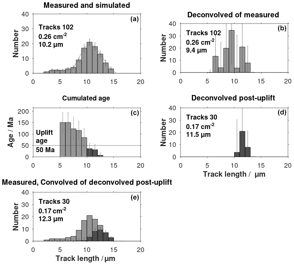
Figure 3(a) The forward-simulated track length histogram resembling a measured histogram, (b) the deconvolved histogram of the measured histogram, and (c) the cumulated age histogram are shown. The dark grey columns identify the post-depositional tracks. Panel (d) shows the post-uplift columns of the deconvolved histogram. (e) The convolution (spreading out) of the deconvolved post-uplift histogram is like the post-uplift part (dark grey) of a measured track length histogram.
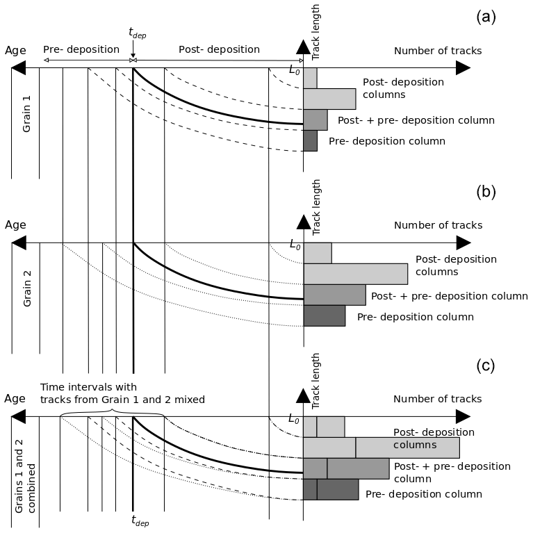
Figure 4Sketch of the accumulation of simplified tracks in histogram columns. All tracks start with the length L0. Some tracks are generated before deposition and some after. The actual track lengths are reduced as a function of time. Panels (a) and (b) show Grain 1 and Grain 2 respectively, which have experienced a different pre-depositional thermal histories. Panel (c) displays the histogram for the bulk of grains 1 and 2.
The deconvolution technique can be used to extract the post-depositional part of track length histograms with inherited tracks. This is illustrated in Fig. 4 using a simplified model for track annealing and observation. Grains from two source areas are considered. There are more tracks in the post-depositional columns of Grain 2 than in Grain 1 because it is assumed that the uranium content of Grain 2 is twice that of Grain 1. The two post-depositional columns of grains 1 and 2 represent the same two time intervals. For both grains 1 and 2, there is one column where pre-and post-depositional tracks are mixed. This column and the pre-depositional columns of both grain types do not necessarily represent the same time intervals because their different thermal histories create individual track length distributions (histograms). The pre-depositional tracks of Grain 1 compared with those of Grain 2 have experienced different thermal histories and, therefore, different degree of annealing. Post-depositional tracks are ordered with decreasing length as a function of time, in contrast to pre-depositional tracks which may be disordered. Figure 4c sums the histograms for grains 1 and 2. It is observed that the post-depositional time intervals for the bulk histogram are identical to those for the two separate grain types. The age equation, Eq. (44), is valid for post-depositional corrected tracks but not for mixed or pre-depositional tracks.
The post-depositional part of the deconvolved histogram ![]() is the columns with track ages tp less than the deposition age tdep:
is the columns with track ages tp less than the deposition age tdep:
where p is the column number. Together with Eq. (44), we obtain
The values of p satisfying the inequality identify the post-sedimentary columns. The smallest number of p identifies the oldest post-sedimentary track. This number is used to calculate the surface track density σpost linked to the post-depositional histogram with Eq. (46):
Summations are performed for all columns representing the post-sedimentary history. Together with the surface track density σpost, the post-depositional histogram may be used to calculate the post-depositional thermal history by applying the backward-modelling procedure described by Jensen et al. (1992). Alternatively, the post-depositional deconvolved histogram can be convolved by forward calculation with Eq. (31) and used by random or guided-random search algorithms (Lutz and Omar, 1991; Willett, 1997; Ketcham, 2005; Gallagher, 1995, 2012).
Identification of post-sedimentary fission tracks is exemplified by applying apatites from the sample GGU103113 (Jameson Land, East Greenland). The Middle Jurassic sandstone sample (170 Ma) has the apparent fission-track age of 245 Ma (Hansen et al., 2001). The measured and the deconvolved track length distributions are shown in Fig. 5a and b respectively.
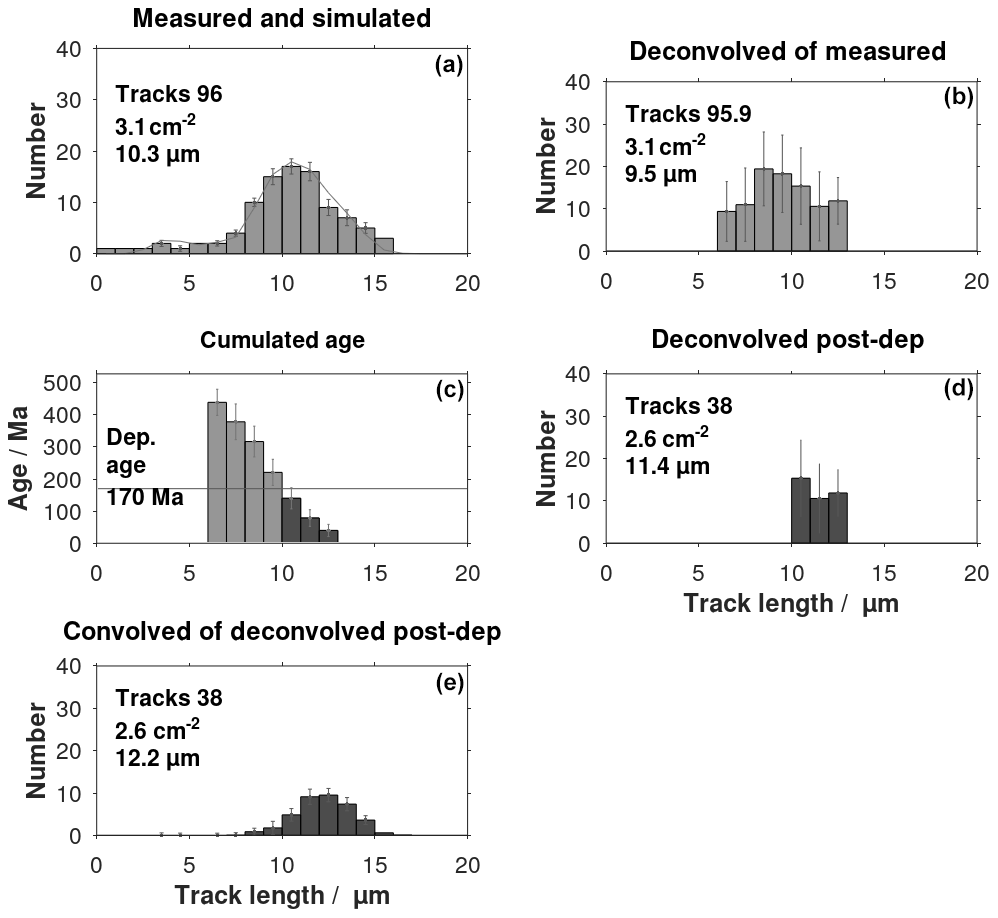
Figure 5Extraction of the post-sedimentary part of a track length histogram from Jameson Land, East Greenland (Hansen, 1996). The surface track density is given in units of per square centimetre Panel (a) shows the measured and simulated (thin line) fission-track length histogram, and panel (b) shows the histogram after deconvolution using the filters shown in Appendix B. (c) The ages of the corrected track are calculated by Eq. (44) using the deconvolved histogram. The columns (dark grey) with ages of corrected tracks that are less than the deposition age (170 Ma) are identified. (d) The post-sedimentary histogram is extracted from the deconvolved histogram based on the identified post-depositional columns. This histogram is the basis for the direct calculation of the temperature history (Jensen et al., 1992). (e) The convolved post-sedimentary histogram, resembling a measured histogram, can be used by Monte Carlo-type simulation models (Ketcham, 2005; Gallagher, 1995).
The parameter ξ in the age equation, Eq. (44), is adjusted to 0.752 (with b=0.784) to obtain a simulated apparent age equal to the apparent age reported by Hansen et al. (2001). The apparent age is calculated using a track length distribution of an unannealed track length distribution in Eq. (44). The post-depositional columns are identified as being the columns on the right with accumulated ages of corrected tracks that are less than the deposition age (Fig. 5c, d). The deconvolved histogram (Fig. 5d) can be used to calculate the post-sedimentary thermal history. The histogram in Fig. 5e is the convolution of the histogram in Fig. 5d.
The equations for accumulated fission tracks derived here are based on the practice of selecting horizontal tracks for length measurements. We follow the recommendation of Ketcham (2019), who selected all tracks within of the horizontal. Alternatively, Gleadow et al. (1986b) and Galbraith (2005) selected tracks observed as being within of the horizontal under reflected light and as having both ends in focus under transmitted light. Fewer long tracks (>8.5 µm) are then selected relative to shorter tracks (Appendix D). An alternative set of equations is given in Appendix D for this situation.
Standard deviations of the ages are calculated based on the variance in input data, the prior model, and modelization. The calculated deviations are high, but they agree with the deviations of histograms reported in an inter-laboratory comparison (Ketcham et al., 2009). It is required that the laboratory-annealed tracks are measured in the same way as the natural tracks. For example, in the Jameson Land instance, the recommendations by Gleadow et al. (1986b, 2019) are used in both cases.
The inversion procedure by Tarantola (2005) requires a prior model that is independent of data. As the default, a prior model histogram with an equal number of tracks in the columns is chosen. In some cases, negative track length histogram columns appear because of inversion due to unrealistic data. An improved prior model based on other information is then necessary. The problem can also be managed by smoothing input data and/or covariance matrices. Another approach to be examined is the Gaussian approximation of the Poisson distribution (Calvetti and Somersalo, 2007).
The stability of the inversions in Eq. (24) depends on the condition numbers for CD, CH, and , which should be less than 105…106. Application of the Octave function cond (Eaton et al., 2020) for the 2D and 3D examples in this paper shows numbers less than 105…106, indicating stability. Refined binning of the histograms may lead to large and possible unstable inversions. In those cases, CD and CH in Eqs. (23) and (24) as well as in Eq. (24) should be replaced by the Cholesky factorized matrixes (see e.g. Cheney and Kincaid, 2008). It is then required that the matrixes are symmetric and positive definite. It is seen from Eqs. (25)–(29) that the matrixes CD and CH are symmetric. The matrix in Eq. (24) is symmetric as well. Application of the Octave function chol (Eaton et al., 2020) shows that the matrixes are positive definite. Therefore, the three matrixes can be Cholesky factorized.
When track angles to the c axis are available, it is common practice to calculate the histogram of the c-axis-projected tracks. However, detailed information on track density is lost during the accumulation along the projection path. Instead, one can use 3D track length histograms, as described in Appendix E. The 3D histograms do not involve projections and, therefore, retain both length and angle information. The inversion procedure presented here is valid for both 2D histograms and 3D histograms (Appendix E).
As an example, the deconvolution method presented here is used to identify the post-depositional part of a track length histogram from Jameson Land, Greenland. A new procedure for deriving ages of corrected fission tracks as a function of track length is suggested. The natural fission-track length histogram is considered to be linearly composed of histograms of induced tracks that are partially annealed in the laboratory. Inversion is performed by a probabilistic inverse theory. The resulting ages of corrected tracks are given as centres of the posterior with variance. The equations are valid for old-type measurements, where the track angle to the c axis is not measured as well as for recent data, including measurements of the angle to the c axis. Data with both track lengths and angles are organized in 3D histograms and presented as images. Two types of track length measurements are discussed. If tracks with both ends in focus are selected, there is a tendency to omit longer tracks. If all tracks within a given angle are selected, this bias disappears. The equations presented here are prepared for both cases. The calculation of the ages of corrected tracks does not require the calculation of the sample thermal history. Instead, they are the basis for temperature history calculation.
After the formation of the unetched randomly oriented tracks, the spreading of lengths increases during the process of annealing, leading to a considerable mixing of lengths of the observed track length histogram. There is not a unique relationship between time and the length of individual tracks. However, the relationship is not completely blurred. There is a tendency for old tracks to appear in the short track length part of the histogram and young tracks to appear in the opposite part. To some extent, deconvolution can reduce the spread. Deconvolution is used extensively in seismic processing to improve the signal-to-noise ratio and remove biases. This requires the character of the noise to be known. The “noise” in connection with fission tracks is the spread observed in laboratory annealing experiments. This is used to reduce the spread of the observed track length histograms; that is, the observed histogram can be deblurred by deconvolution. A simplified demonstration of the deconvolution of a bimodal track length histogram is shown in Fig. A1. The present paper applies a more advanced least-squares deconvolution technique.
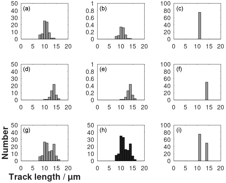
Figure A1Illustration of deconvolution of a track length histogram. The dark grey histogram in panel (h) is the observed histogram. The histogram in panel (i) is an initial guess of a deconvolved histogram with 80 and 50 tracks in each column. The histograms in panels (f) and (c) are the two columns of the histogram in panel (h) separated. The histograms in panels (b) and (e) are normalizations of histograms observed after track annealing in the laboratory. They are named filters. The histogram in panel (a) is the histogram in panel (b) multiplied by the number of tracks in the histogram in panel (c). The histogram in panel (d) is the histogram in panel (e) multiplied by the number of tracks in the histogram in panel (f). The histogram in panel (g) is the histogram in panel (a) plus the histogram in panel (d). The histogram in panel (g) is then the result of the convolution of the histogram in panel (i) with the filters in panels (b) and (e). The synthetic histogram in panel (g) is compared with the observed histogram in panel (h); however, the left part is dissimilar. Therefore, the suggested deconvolved histogram in panel (i) is not successful.
A successful deconvolution is shown in Fig. A2. The spread of tracks in the bimodal histogram in Fig. A2h is assembled in two columns corresponding to two thermal time periods. Note that the two time periods can be separated despite the track length overlap of the histograms in Fig. A2a and d. The deconvolved track length histogram in Fig. A2i is arranged according to time. Each column can be converted to an equivalent time interval. The age of the oldest track of each column of deconvolved histograms is calculated by adding its associated time interval and younger time intervals. During this process, there was no use of a track annealing model.
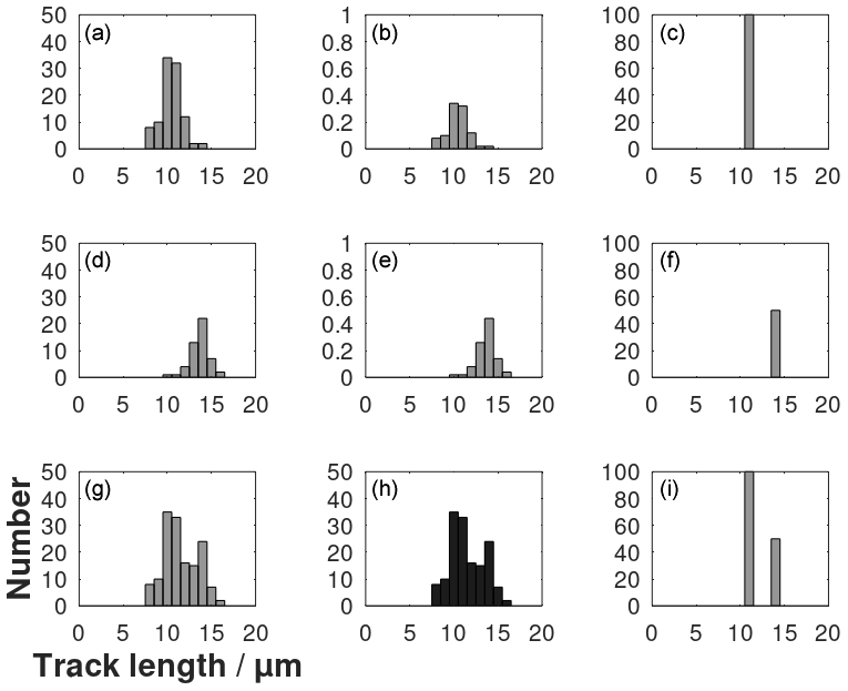
Figure A2The final step of the deconvolution procedure showing the successful deconvolution of the histogram in panel (h). The histogram in panel (i) is the deconvolved histogram. The degree of success is measured by comparing the convolved histograms in panels (g) and (h).
The filters used for deconvolution are the columns of matrix G (Eq. 22). They are based on measurements of track lengths after annealing in the laboratory (Gleadow et al., 1986a; Green et al., 1986; Barbarand et al., 2003). The histograms of these track lengths are normalized using division by the number of tracks of each histogram. They represent the probability of an induced track appearing in a certain length interval. Interpolated filters are obtained using a mesh of 0.2 µm in both directions (bins and mean track lengths) (Fig. B1).
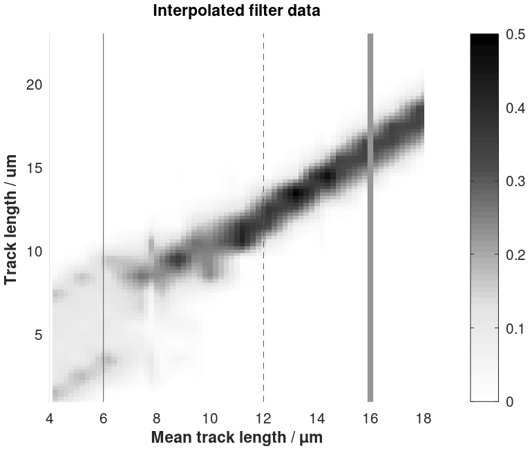
Figure B1Interpolation of the filters used for deconvolution. It is based on track annealing in the laboratory (Gleadow et al., 1986a; Green et al., 1986; Barbarand et al., 2003). Three linear intersections are shown in Fig. B2. The greyscale range denotes frequency.
The filters broaden with decreasing mean track length. The columns of the modelization matrix G are picked from the interpolation. The number of columns is related to the resolution. Figure B2 shows three filters extracted from Fig. B1.
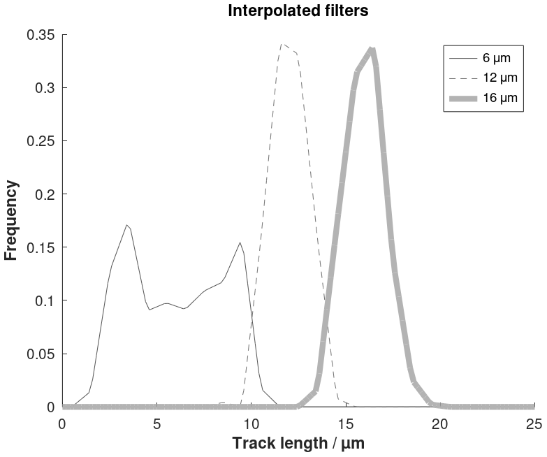
Figure B2Three interpolated filters with mean track lengths of 6, 12, and 15 µm extracted from Fig. B1.
Plots of mean track length versus surface track density for tracks generated by neutron radiation and annealed in the laboratory are given by Green et al. (1986). A logarithmic expression approximates data (Fig. C1):
where is the surface track density of partially annealed tracks relative to that of unannealed tracks. is the mean track length of partially annealed tracks relative to the unannealed mean track length. Equation (C1) is used to parameterize the measured data leading to for multi-compositional apatite and b=0.963 for mono-compositional apatite. b determines the curvature of the approximating line in Fig. C1.
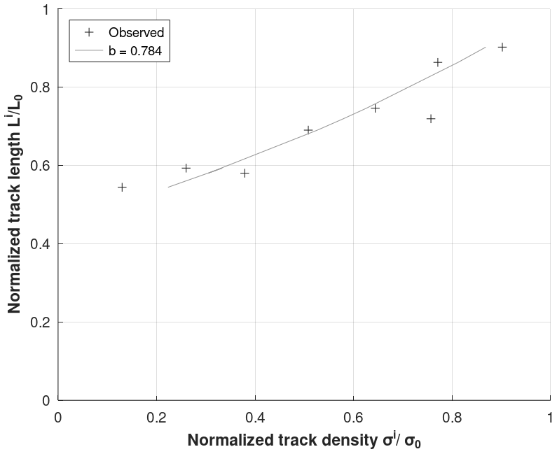
Figure C1Parameter b characterizes the relation between normalized track length and normalized density for multi-compositional apatite. Data are from Green (1988).
Ketcham (2019) recommended the selection of all etched tracks within of the horizontal. It is expected that the likelihood of tracks being etched is proportional to their length. This view has been adopted in the main text of this paper. Alternatively, the selection criteria of Ketcham (2019) and Gleadow et al. (2019) focused on etched tracks that are within 10–15∘ of the horizontal and that have both ends in focus at the same time. The two criteria are examined in this appendix.
The axial (vertical) resolution of a light microscope is
With typical values for a wavelength of λ=550 nm (green light), the refraction index of oil of η=1.51, and a numerical aperture of NA=1.25, the axial resolution raxial=0.74 µm. The numerical aperture is a measure of the maximum angle for which the microscope receives light. The criteria by Gleadow et al. (2019) imply that a short track (6 µm long) is accepted for counting if the angle to the horizontal is less than 10∘. A long track (18 µm) must be within 2.5∘ of the horizontal to be accepted. Therefore, the tendency is that long tracks are omitted from counting. The likelihood of selection is then inversely proportional to the track length for tracks longer than 6 µm. At the same time, the likelihood of a horizontal track being etched is expected to be proportional to its length. These two biases essentially cancel each other (Jensen et al., 1992). With the focus window selection criteria (Gleadow et al., 2019), the set of age equations is then
The age of the oldest track is obtained by summing all of the time intervals:
Introducing the mean track length of the inverted histogram ![]() ,
,
The age of the oldest observable track is
which is equivalent to the derivation by Jensen et al. (1992) when ℒmean is replaced by the mean track length.
The inversion principle presented in the main text is for 2D track length histograms ignoring track angles to the c axis. However, the inversion principle is also applicable to data that include the angles. The measured data vector dobs in Eq. (24) is then derived from a 3D histogram (length, angle, and number). The elements of the vector dobs are obtained by sequentially numbering each bin (Tarantola, 2005).
An example is shown in Fig. E1 using a synthetic 3D histogram of data obtained from two annealing experiments. These data are the result of heating to 275 and 320 ∘C respectively (Barbarand et al., 2003). Each bin of the 3D histogram is . The matrix G, Eq. (22), consists of twenty 3D filters interpolated between the six annealing experiments by Barbarand et al. (2003). Each column of G is a filter. Two of them are shown in Fig. E2. The corrected histogram as a result of the inversion using Eq. (24) is shown in Fig. E3.
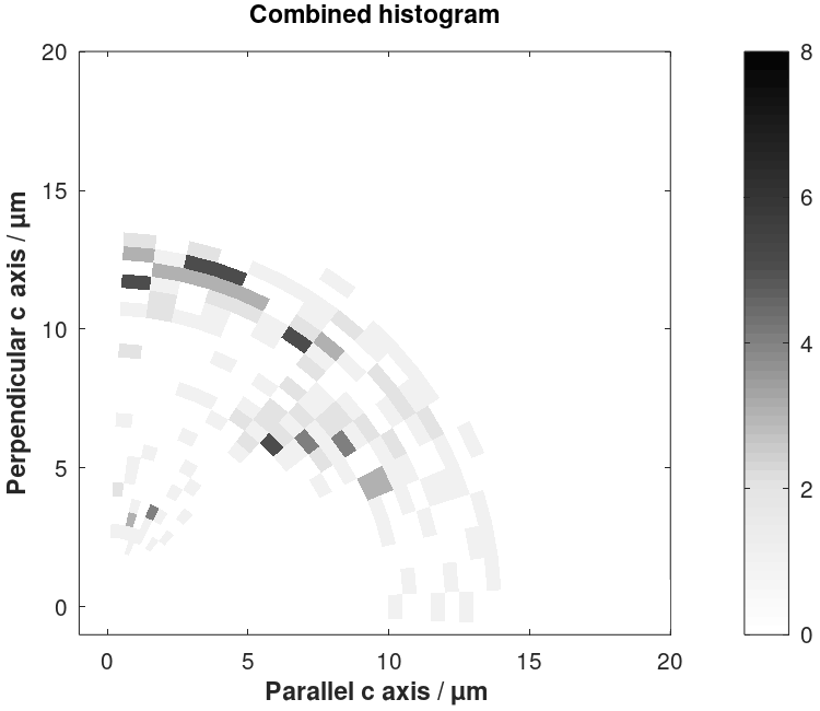
Figure E1A 3D histogram of track lengths versus angles derived by combining two annealing experiments (Barbarand et al., 2003). The greyscale range denotes the number of tracks in each bin.
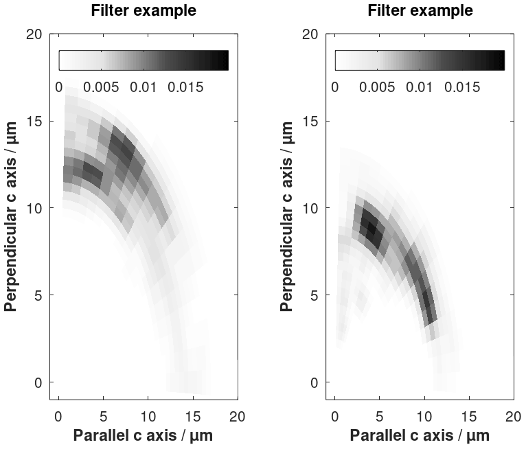
Figure E2Examples of 3D filters used for deconvolution. They are based on heating to 275 and 320 ∘C respectively (Barbarand et al., 2003). The greyscale range denotes frequency.
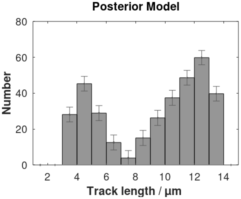
Figure E3The corrected histogram as a result of the inversion of the 3D histogram shown in Fig. E1.
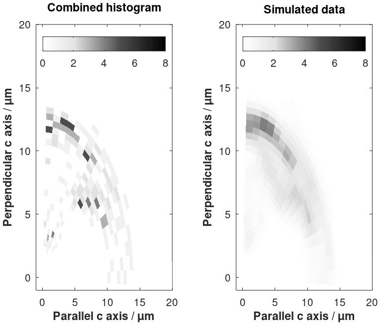
Figure E4The combined 3D histogram considered as synthetic data (Fig. E1) and the forward-simulated approximation using the posterior model in Eq. (24). The greyscale range denotes the number of tracks.
The standard deviations are the diagonal values of the posterior covariance matrix. The result of the inversion is evaluated by comparing forward modelling using Eq. (21) with the inverted histogram as input data (Fig. E3). Compliance is good (Fig. E4).
Octave (Eaton et al., 2020; https://ftpmirror.gnu.org/octave; last access: 12 December 2021) codes for reproducing the results shown in Figs. B1, B2, and E1–E4 are available on Zenodo at https://doi.org/10.5281/zenodo.5595057 (Jensen, 2021a) and https://doi.org/10.5281/zenodo.5595075 (Jensen, 2021b) for 2D histograms and 3D histograms respectively.
PKJ developed the theory. During this process, discussions with KH were important. PKJ wrote the equations and the computer programmes; he also wrote the paper in tight dialogue with KH. KH measured the track lengths and surface track density used in the example shown in Fig. 5.
The contact author has declared that neither they nor their co-author has any competing interests.
Publisher’s note: Copernicus Publications remains neutral with regard to jurisdictional claims in published maps and institutional affiliations.
This paper was edited by Shigeru Sueoka and reviewed by Raymond Donelick, Paul Green, and one anonymous referee.
Afra, B., Lang, M., Rodriguez, M. D., Zhang, J., Giulian, R., Kirby, N., Ewing, R. C., Trautmann, C., Toulemonde, M., and Kluth, P.: Annealing kinetics of latent particle tracks in Durango apatite, Phys. Rev. B, 83, 064116, https://doi.org/10.1103/PhysRevB.83.064116, 2011.
Barbarand, J., Hurford, T., and Carter, A.: Variation in apatite fission-track length measurement: implications for thermal history modelling, Chem. Geol., 198, 77–106, https://doi.org/10.1016/S0009-2541(02)00423-0, 2003.
Bardsley, J. M.: Computational uncertainty quantification for inverse problems, SIAM, Philadelphia, 19, 133 pp., ISBN: 1611975379 and 9781611975376, 2018.
Bertagnolli, E., Keil, R., and Pahl, M.: Thermal history and length distribution of fission tracks in apatite, Part I., Nucl. Tracks Rad. Meas., 7, 163–177, https://doi.org/10.1016/0735-245X(83)90026-1, 1983.
Calvetti, D. and Somersalo, E.: An introduction to Bayesian scientific computing: ten lectures on subjective computing, Vol. 2. Springer Science & Business Media, Springer+Business Media, New York, 202 pp., ISBN: 78-0-387-73393-7, 2007.
Cheney, E. W. and Kincaid, D. R.: Numerical mathematics and computing, Cengage Learning, Bob Pirtle, USA, ISBN-13: 978-0-495-11475-8, 2008.
Donelick, R. A.: Etchable fission track length distribution in apatite: experimental observations, theory and geological applications, PhD dissertation, Rensselaer Polytechnic Institute, Troy, New York, 414 pp., 1988.
Donelick, R. A., Ketcham, R. A., and Carlson, W. D.: Variability of apatite fission-track annealing kinetics: II. Crystallographic orientation effects, Am. Mineral., 84, 1224–1234, https://doi.org/10.2138/am-1999-0902, 1999.
Eaton, J. W., Bateman, D., Hauberg, S., and Wehbring, R.: GNU Octave version 6.1.0 manual: a high-level interactive language for numerical computations, GNU [code], available at: https://ftpmirror.gnu.org/octave (last access: 12 December 2021), 2020.
Fleischer, R. L., Price, P. B., and Walker, R. M.: Nuclear Tracks in Solids: Principles and Applications, University of California Press, Berkeley, CA, 605 pp., 1975.
Galbraith, R. F.: Statistics for fission track analysis, Chapman and Boca Raton, 240 pp., ISBN 9780367392796, 2005.
Gallagher, K.: Evolving temperature histories from apatite fission-track data, Earth Planet. Sci. Lett., 136, 421–435, https://doi.org/10.1016/0012-821X(95)00197-K, 1995.
Gallagher, K.: Transdimensional inverse thermal history modeling for quantitative thermochronology, J. Geophys. Res., 117, B02408, https://doi.org/10.1029/2011JB008825, 2012.
Gleadow, A., Kohn, B., and Seiler, C.: The Future of Fission-Track Thermochronology, in: Fission-Track Thermochronology and its Application to Geology, edited by: Malusà, M. and Fitzgerald, P., Springer Textbooks in Earth Sciences, Geography and Environment, Springer, Cham, https://doi.org/10.1007/978-3-319-89421-8_4, 2019.
Gleadow, A. J. W., Duddy, I. R., Green, P. F., and Hegarty, K. A.: Fission track lengths in the apatite annealing zone and the interpretation of mixed ages, Earth Planet. Sci. Lett., 78, 245–254, https://doi.org/10.1016/0012-821X(86)90065-8, 1986a.
Gleadow, A. J. W., Duddy, I. R., Green, P. F., and Lovering, J. F.: Confined fission track lengths in apatite: a diagnostic tool for thermal history analysis, Contrib. Mineral. Petr., 94, 405–415, https://doi.org/10.1007/BF00376334, 1986b.
Green, P. F.: The relationship between track shortening and fission track age reduction in apatite: combined influences of inherent instability, annealing anisotropy, length bias and system calibration, Earth Planet. Sci. Lett., 89, 335–352, https://doi.org/10.1016/0012-821X(88)90121-5, 1988.
Green, P. F., Duddy, I. R., Gleadow, A. J. W., Tingate, P. R., and Laslett, G. M.: Thermal annealing of fission tracks in apatite: 1. A qualitative description, Chem. Geol.: Isotope Geoscience section, 59, 237–253, https://doi.org/10.1016/0168-9622(86)90074-6, 1986.
Green, P. F., Duddy, I. R., Laslett, G. M., Hegarty, K. A., Gleadow, A. J. W., and Lovering, J. F.: Thermal annealing of fission tracks in apatite 4. Quantitative modelling techniques and extension to geological timescales, Chem. Geol.: Isotope Geoscience section, 79, 155–182, https://doi.org/10.1016/0168-9622(89)90018-3, 1989.
Hansen, K.: Thermotectonic evolution of a rifted continental margin: fission track evidence from the Kangerlussuaq area, SE Greenland, Terra Nova, 8, 458–469, https://doi.org/10.1111/j.1365-3121.1996.tb00771.x, 1996.
Hansen, K., Bergman, S. C., and Henk, B.: The Jameson Land basin (east Greenland): a fission track study of the tectonic and thermal evolution in the Cenozoic North Atlantic spreading regime, Tectonophysics, 331, 307–339, https://doi.org/10.1016/S0040-1951(00)00285-7, 2001.
Jensen, P. K.: Deconvolution of 2D-fission track length histograms, Zenodo [code, dataset], https://doi.org/10.5281/zenodo.5595057, 2021a.
Jensen, P. K.: Deconvolution of 3D-fission track length histograms, Zenodo [code, dataset], https://doi.org/10.5281/zenodo.5595075, 2021b.
Jensen, P. K. and Hansen, K.: Identifying the post-sedimentary part of fission track length histograms with inherited tracks, Thermo 2018, 16th International Conference on Thermochronology, Quedlinburg, Germany, 16–21 September 2018, https://doi.org/10.1002/essoar.10500031.1, 2018.
Jensen, P. K., Hansen, K., and Kunzendorf, H.: A numerical model for the thermal history of rocks based on confined horizontal fission tracks. International Journal of Radiation Applications and Instrumentation. Part D. Nuclear Tracks and Radiation Measurements, 20, 349–359, https://doi.org/10.1016/1359-0189(92)90064-3, 1992.
Jensen, P. K., Bidstrup, T., Hansen, K., and Kunzendorf, H.: The Use of Fission Track Measurements in Basin Modeling, in: Computerized Basin Analysis, edited by: Harff, J. and Merriam, D. F., Springer US, https://doi.org/10.1007/978-1-4615-2826-5_7, 1993.
Jungerman, J. and Wright, S. C.: Kinetic Energy Release in Fission of U238, U235, Th232, and Bi209 by High Energy Neutrons, Phys. Rev., 76, 1112–1116, https://doi.org/10.1103/PhysRev.76.1112, 1949.
Keil, R., Pahl, M., and Bertagnolli, E.: Thermal history and length distribution of fission tracks: Part II, International Journal of Radiation Applications and Instrumentation. Part D. Nuclear Tracks and Radiation Measurements, 13, 25–33, 1987.
Ketcham, R. A.: Observations on the relationship between crystallographic orientation and biasing in apatite fission-track measurements, Am. Mineral., 88, 817–829, https://doi.org/10.2138/am-2003-5-610, 2003.
Ketcham, R. A.: Forward and inverse modeling of low-temperature thermochronometry data, Rev. Mineral. Geochem., 58, 275–314, https://doi.org/10.2138/rmg.2005.58.11, 2005.
Ketcham, R. A.: Fission-Track Annealing: From Geologic Observations to Thermal History Modeling, in: Fission-Track Thermochronology and its Application to Geology, edited by: Malusà, M. and Fitzgerald, P., Springer Textbooks in Earth Sciences, Geography and Environment, Springer, Cham., https://doi.org/10.1007/978-3-319-89421-8_3, 2019.
Ketcham, R. A., Donelick, R. A., Balestrieri, M. L., and Zattin, M.: Reproducibility of apatite fission-track length data and thermal history reconstruction, Earth Planet. Sci. Lett., 284, 504–515, https://doi.org/10.1016/j.epsl.2009.05.015, 2009.
Kirkpatrick, S., Gelatt, C. D., and Vecchi, M. P.: Optimization by simulated annealing, Science, 220, 671–680, https://doi.org/10.1126/science.220.4598.671, 1983.
Laslett, G. M., Gleadow, A. J. W., and Duddy, I. R.: The relationship between fission track length and track density in apatite, Nucl. Tracks Rad. Meas., (1982), 9, 29–38, https://doi.org/10.1016/0735-245X(84)90019-X, 1984.
Li, W., Wang, L., Lang, M., Trautmann, C., and Ewing, R. C.: Thermal annealing mechanisms of latent fission tracks: Apatite vs. zircon, Earth Planet. Sci. Lett., 302, 227–235, https://doi.org/10.1016/j.epsl.2010.12.016, 2011.
Lutz, T. M. and Omar, G.: An inverse method of modeling thermal histories from apatite fission-track data, Earth Planet. Sci. Lett., 104, 181–195, https://doi.org/10.1016/0012-821X(91)90203-T, 1991.
Stephenson, J., Gallagher, K., and Holmes, C.: A Bayesian approach to calibrating apatite fission track annealing models for laboratory and geological timescales, Geochim. Cosmochim. Ac., 70, 5183–5200, https://doi.org/10.1016/j.gca.2006.07.027, 2006.
Tarantola, A.: Inverse problem theory, SIAM, Philadelphia, https://doi.org/10.1137/1.9780898717921, 2005.
Willett, S. D.: Inverse modeling of annealing of fission tracks in apatite; 1, A controlled random search method, Am. J. Sci., 297, 939–969, https://doi.org/10.2475/ajs.297.10.939, 1997.
- Abstract
- Overview of the formation of fission tracks
- Summary of age and temperature calculation
- Correcting for biases in track length histograms using deconvolution
- Equations for the age distribution of corrected tracks
- Variance in ages
- Testing the deconvolution method
- Inherited tracks
- Discussion
- Conclusions
- Appendix A
- Appendix B
- Appendix C
- Appendix D
- Appendix E
- Code and data availability
- Author contributions
- Competing interests
- Disclaimer
- Review statement
- References