Short communication: On the potential use of materials with heterogeneously distributed parent and daughter isotopes as primary standards for non-U–Pb geochronological applications of laser ablation inductively coupled plasma mass spectrometry (LA-ICP-MS)

Many new geochronological applications of laser ablation inductively coupled plasma mass spectrometry (LA-ICP-MS) have been proposed in recent years. One of the problems associated with this rapid growth is the lack of chemically and isotopically homogeneous matrix-matched primary standards to control elemental fractionation during LA-ICP-MS analysis. In U–Pb geochronological applications of LA-ICP-MS this problem is often addressed by utilising matrix-matched primary standards with variable chemical and isotopic compositions. Here I derive a set of equations to adopt this approach for non-U–Pb geochronological applications of LA-ICP-MS.

1 Introduction

The use of laser ablation inductively coupled plasma mass spectrometry (LA-ICP-MS) for in situ geochronology is growing rapidly, and recent years have seen this technique being applied to many new minerals and isotope systems. Examples include in situ U–Pb dating of apatite (Chew et al., 2014, 2011), carbonates (Roberts et al., 2017; Li et al., 2014; Guillong et al., 2020) and epidote (Peverelli et al., 2021), Rb–Sr dating of micas (Hogmalm et al., 2017; Zack and Hogmalm, 2016), alkali feldspar (Bevan et al., 2021) and celadonite (Laureijs et al., 2021), Lu–Hf dating of garnet, apatite and xenotime (Simpson et al., 2021), and a new approach to Re–Os dating of molybdenite (Hogmalm et al., 2019). One important challenge associated with this rapid growth is the development of matrix-matched primary standards to correct for elemental fractionation during LA-ICP-MS analysis. Ideally, primary standards should be chemically and isotopically homogeneous and isostructural to the analysed minerals. However, finding or synthesising such materials is not trivial. Therefore, recent studies have relied on some alternative solutions, including the use (i) matrix-matched standards with variable chemical and isotopic composition (e.g. Chew et al., 2014) and (ii) nanoparticulate pressed powder tablets as substitutes for chemically and isotopically homogeneous matrix-matched standards (e.g. Hogmalm et al., 2017).

Matrix-matched primary standards with variable contents of parent and daughter isotopes are often used in U–Pb geochronological applications of LA-ICP-MS. Chew et al. (2014) proposed several approaches for dating common-Pb-bearing phases, in which primary standards with variable contents of common Pb are used to characterise U–Pb fractionation. In all of these, individual primary-standard analyses are corrected for common Pb before factors to correct for U–Pb fractionation are calculated from them, such that the latter step only relies on comparing the observed and expected ${}^{\mathrm{238}}\mathrm{U}{/}^{\mathrm{206}}{\mathrm{Pb}}_{\mathrm{radiogenic}}$ ratios (as opposed to using the ${}^{\mathrm{238}}\mathrm{U}{/}^{\mathrm{206}}{\mathrm{Pb}}_{\mathrm{total}}$ ratios). The approaches differ in how the common-Pb correction is introduced. This can be achieved by using ²⁰⁴Pb or, assuming that no ²³²Th is present, ²⁰⁸Pb to estimate the amounts of common ²⁰⁶Pb and calculate the ${}^{\mathrm{238}}\mathrm{U}{/}^{\mathrm{206}}{\mathrm{Pb}}_{\mathrm{radiogenic}}$ ratios. Alternatively, straight lines can be projected from an a priori estimate for the initial ${}^{\mathrm{207}}\mathrm{Pb}{/}^{\mathrm{206}}\mathrm{Pb}$ ratio through the acquired U–Pb data to the concordia in the Tera–Wasserburg space to calculate the ${}^{\mathrm{238}}\mathrm{U}{/}^{\mathrm{206}}{\mathrm{Pb}}_{\mathrm{radiogenic}}$ ratios (Fig. 1a). A similar approach was adopted by Li et al. (2014), Roberts et al. (2017) and Guillong et al. (2020), who first used chemically and isotopically homogeneous non-matrix-matched primary standards to correct for any drift in U–Pb fractionation during analytical sessions and then used matrix-matched primary standards with variable contents of common Pb to calculate correction factors for matrix-dependent U–Pb fractionation. The latter was done by plotting multiple primary-standard analyses in the Tera–Wasserburg diagram to fit a straight line through them and compare its observed and expected intercepts with the concordia.

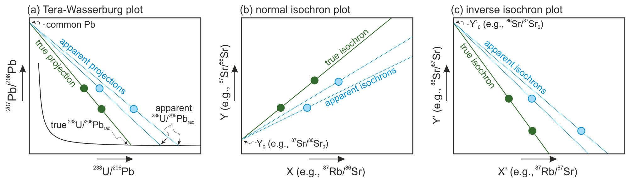
Figure 1 Schematic illustrations for how individual analyses of primary standards with variable parent and daughter isotope concentrations can be used to obtain factors for elemental-fractionation correction. Each plot shows two data points that are assumed to be corrected for mass-dependent fractionation and have different elemental-fractionation factors (e.g. due to instrument instability). (a) One of the approaches taken in U–Pb geochronological applications of LA-ICP-MS. Factors for U–Pb fractionation correction are calculated by rationing the true and apparent ${}^{\mathrm{238}}\mathrm{U}{/}^{\mathrm{206}}{\mathrm{Pb}}_{\mathrm{radiogenic}}$ ratios that are obtained using the Tera–Wasserburg diagram. (b–c) Potential approaches for non-U–Pb geochronological applications of LA-ICP-MS. Factors for elemental-fractionation correction can be estimated by finding coefficients by which the measured elemental ratios need to be multiplied to equate the slopes of the apparent and true isochrons, whether normal or inverse. Elemental-fractionation correction factors can also be estimated by comparing the true and apparent intercepts with the horizontal axis in the inverse isochron diagram.

I have found only two non-U–Pb geochronological applications of LA-ICP-MS where materials with variable contents of parent and daughter isotopes were essentially used as a primary standard. The first is the pioneering work on in situ Rb–Sr dating by Zack and Hogmalm (2016). These authors calculated what factor is needed to correct for Rb–Sr fractionation in one biotite sample with known age to obtain an isochron of that age and then applied it to other samples measured on the same day. Another is the work of Bevan et al. (2021), who performed Rb–Sr analysis of two alkali feldspar samples alongside each other and then corrected the data for one of them using the Rb–Sr fractionation factors that were deduced by comparing the observed and expected isochron slopes for the other. Most recent studies have relied on using nanoparticulate pressed powder tablets as substitutes for chemically and isotopically homogeneous matrix-matched primary standards (Hogmalm et al., 2017, 2019; Olierook et al., 2020; Li et al., 2020; Tillberg et al., 2021). However, the ablation properties of nanoparticulate pressed powder tablets are different from those of single crystals, and while they perform better as primary standards compared to glasses, Rb–Sr dates obtained by using them can be offset from the expected values by several percentage points (mostly up to 4 %, occasionally up to 7 % in tests of Redaa et al., 2021). Therefore, the quest for matrix-matched standards remains open. With this communication I aim to highlight that the idea of using materials with heterogeneously distributed parent and daughter isotopes as primary standards may deserve more attention, and I provide a set of equations to implement it.

2 Proposed solution

Presumably, one of the reasons why the idea of using primary standards with variable contents of parent and daughter isotopes was abandoned in non-U–Pb geochronological applications of LA-ICP-MS is the absence of a clear approach to calculate factors for elemental-fractionation correction and their uncertainties. Clearly, these factors can be estimated by adopting one of the approaches used for U–Pb dating. For example, they can be estimated from individual primary-standard analyses by using parent-to-daughter isotope ratios that are corrected for the presence of the non-radiogenic component of the daughter isotope using a common isotope, which is analogous to the aforementioned use of the ²⁰⁴Pb- and ²⁰⁸Pb-based correction methods. Alternatively, they can be estimated by plotting two-point normal or inverse isochrons based on individual primary-standard analyses and finding by what coefficients the measured elemental ratios need to be multiplied to bring the slopes of the apparent normal or inverse isochrons to the true values (Fig. 1b, c). Finally, these factors can be estimated by calculating and comparing the observed and expected intercepts with the horizontal axis in the inverse isochron diagram, which is analogous to the aforementioned use of the Tera–Wasserburg diagram (Fig. 1c). But how to calculate elemental-fractionation correction factors in an efficient way? And how to estimate their uncertainties and propagate these to the date uncertainties? Below I derive equations that can be used to do so. I rely on the uncertainty propagation law (JCGM, 2008), although other approaches exist, such as the method of maximum likelihood (Vermeesch, 2022).

2.1 Normal isochron space

In the normal isochron space, the true composition of a primary standard with heterogeneously distributed parent and daughter isotopes is given by Eq. (1):

$$\begin{array}{}\text{(1)}& Y=Y_{\mathrm{0}}+X\left(e^{\mathit{\lambda }t}-\mathrm{1}\right),\end{array}$$

where Y is the daughter-to-common isotope ratio (e.g. ${}^{\mathrm{87}}\mathrm{Sr}{/}^{\mathrm{86}}\mathrm{Sr}$), Y₀ is the initial daughter-to-common isotope ratio (e.g. ${}^{\mathrm{87}}\mathrm{Sr}{/}^{\mathrm{86}}{\mathrm{Sr}}_{\mathrm{0}}$), X is the parent-to-common isotope ratio (e.g. ${}^{\mathrm{87}}\mathrm{Rb}{/}^{\mathrm{86}}\mathrm{Sr}$), λ is the decay constant and t is the age of the primary standard. The analysis of this primary standard by LA-ICP-MS yields some proxies for the true Y and X values, which are the measured y and x values, respectively. It is generally presumed that any difference between Y and y is a result of mass-dependent fraction that can be corrected for independently of analysing the primary standard in question (e.g. Chew et al., 2011; Li et al., 2014; Hogmalm et al., 2017; Redaa et al., 2021) or by acquiring data for pairs of non-radiogenic isotopes while analysing this primary standard (Bevan et al., 2021). Thus, Y can be assumed to be equal to the product of y and the obtained mass fractionation correction factor l. Any difference in X and x can be described in terms of elemental fractionation, which is heavily dependent on the matrix properties and ablation conditions and which is characterised by analysing the primary standard in question (e.g. Chew et al., 2011; Li et al., 2014; Hogmalm et al., 2017; Redaa et al., 2021). Thus, it can be assumed that X is equal to the product of x and the yet unknown factor k needed to correct for elemental fractionation. With these assumptions Eq. (1) can be modified to make Eq. (2):

$$\begin{array}{}\text{(2)}& ly=Y_{\mathrm{0}}+kx\left(e^{\mathit{\lambda }t}-\mathrm{1}\right),\end{array}$$

from which it is possible to obtain an expression for k given by Eq. (3):

$$\begin{array}{}\text{(3)}& k={\displaystyle \frac{ly-Y_{\mathrm{0}}}{x\left(e^{\mathit{\lambda }t}-\mathrm{1}\right)}}.\end{array}$$

The uncertainty of k calculated in this way can be estimated using Eq. (4):

$$\begin{array}{}\text{(4)}& \begin{array}{rl}{\mathit{\sigma }}_k^{\mathrm{2}}=& {\mathit{\sigma }}_x^{\mathrm{2}}{\left({\displaystyle \frac{-k}{x}}\right)}^{\mathrm{2}}+{\mathit{\sigma }}_y^{\mathrm{2}}{\left({\displaystyle \frac{lk}{yl-Y_{\mathrm{0}}}}\right)}^{\mathrm{2}}+\mathrm{2}{\mathit{\sigma }}_{x,y}\left({\displaystyle \frac{-l{k}^{\mathrm{2}}}{x\left(yl-Y_{\mathrm{0}}\right)}}\right)\\ & +{\mathit{\sigma }}_t^{\mathrm{2}}{\left({\displaystyle \frac{-\mathit{\lambda }k}{\mathrm{1}-e^{-\mathit{\lambda }t}}}\right)}^{\mathrm{2}}+{\mathit{\sigma }}_{\mathit{\lambda }}^{\mathrm{2}}{\left({\displaystyle \frac{-tk}{\mathrm{1}-e^{-\mathit{\lambda }t}}}\right)}^{\mathrm{2}}\\ & +\mathrm{2}{\mathit{\sigma }}_{\mathit{\lambda },t}\left({\displaystyle \frac{t\mathit{\lambda }{k}^{\mathrm{2}}}{{\left(\mathrm{1}-e^{-\mathit{\lambda }t}\right)}^{\mathrm{2}}}}\right)+{\mathit{\sigma }}_l^{\mathrm{2}}{\left({\displaystyle \frac{yk}{yl-Y_{\mathrm{0}}}}\right)}^{\mathrm{2}}\\ & +{\mathit{\sigma }}_{Y_{\mathrm{0}}}^{\mathrm{2}}{\left({\displaystyle \frac{-k}{yl-Y_{\mathrm{0}}}}\right)}^{\mathrm{2}}+\mathrm{2}{\mathit{\sigma }}_{Y_{\mathrm{0}},t}\left({\displaystyle \frac{\mathit{\lambda }x{k}^{\mathrm{3}}{e}^{\mathit{\lambda }t}}{{\left(yl-Y_{\mathrm{0}}\right)}^{\mathrm{2}}}}\right),\end{array}\end{array}$$

where only the first three terms should be used to calculate the internal uncertainty (σ_k int) and the entire equation should be used to calculate the external uncertainty (σ_k ext). In principle, ${\mathit{\sigma }}_{Y_{\mathrm{0}},t}$ and σ_λ,t should be different from zero if t was determined using the same Y₀ and λ as in the equations above (i.e. the age of the primary standard is not determined using some other method). Provided that this is the case, ${\mathit{\sigma }}_{Y_{\mathrm{0}},t}$ and σ_λ,t can be estimated using Eqs. (5)–(6):

$$\begin{array}{}\text{(5)}& {\mathit{\sigma }}_{\mathit{\lambda },t}=-{\displaystyle \frac{t{\mathit{\sigma }}_{\mathit{\lambda }}^{\mathrm{2}}}{\mathit{\lambda }}},\end{array}$$

$$\begin{array}{}\text{(6)}& {\mathit{\sigma }}_{Y_{\mathrm{0}},t}=-{\displaystyle \frac{{\mathit{\sigma }}_{Y_{\mathrm{0}}}^{\mathrm{2}}}{\mathit{\lambda }{X}^{\ast }{e}^{\mathit{\lambda }t}}}={\displaystyle \frac{{\mathit{\sigma }}_{Y_{\mathrm{0}}}^{\mathrm{2}}{\mathit{\eta }}^{\ast }}{\mathit{\lambda }{e}^{\mathit{\lambda }t}}},\end{array}$$

where X^∗ is the parent-to-common isotope ratio used to determine t if it was determined from a single analysis, while η^∗ is the partial derivative of the isochron slope with respect to Y₀ if t was determined by fitting an isochron. I show in Appendix A how to calculate η^∗ if the isochron was fitted by the method of York et al. (2004). Note that for well-characterised primary standards, ${\mathit{\sigma }}_{Y_{\mathrm{0}},t}$ will most likely be negligibly small. It is also likely that the contribution from the uncertainties in l and Y₀ to the uncertainty in k will be negligibly small.

Repeated primary-standard analyses will yield k₁ to k_N, for which the weighted mean value k_wm can be obtained via Eq. (7):

$$\begin{array}{}\text{(7)}& k_{\mathrm{wm}}={\displaystyle \frac{{\sum }_{\mathrm{1}}^N{k}_i{w}_i}{{\sum }_{\mathrm{1}}^N{w}_i}},\end{array}$$

where $w_i={\mathit{\sigma }}_{k_i\mathrm{int}}^{-\mathrm{2}}$.

The uncertainty of k_wm is given by Eq. (8):

$$\begin{array}{}\text{(8)}& \begin{array}{rl}{\mathit{\sigma }}_{k_{\mathrm{wm}}}^{\mathrm{2}}=& {\displaystyle \frac{\mathrm{1}}{{\sum }_{\mathrm{1}}^N{w}_i}}+{\mathit{\sigma }}_{\mathit{\lambda }}^{\mathrm{2}}{\left({\displaystyle \frac{t{k}_{\mathrm{wm}}}{e^{-\mathit{\lambda }t}-\mathrm{1}}}\right)}^{\mathrm{2}}+{\mathit{\sigma }}_t^{\mathrm{2}}{\left({\displaystyle \frac{\mathit{\lambda }{k}_{\mathrm{wm}}}{e^{-\mathit{\lambda }t}-\mathrm{1}}}\right)}^{\mathrm{2}}\\ & +\mathrm{2}{\mathit{\sigma }}_{\mathit{\lambda },t}\left({\displaystyle \frac{t\mathit{\lambda }{k}_{\mathrm{wm}}^{\mathrm{2}}}{{\left(e^{-\mathit{\lambda }t}-\mathrm{1}\right)}^{\mathrm{2}}}}\right)\\ & +{\mathit{\sigma }}_l^{\mathrm{2}}{\left({\displaystyle \frac{k_{\mathrm{wm}}}{l}}+{\displaystyle \frac{Y_{\mathrm{0}}}{l\left(e^{\mathit{\lambda }t}-\mathrm{1}\right){\sum }_{\mathrm{1}}^N{w}_i}}{\sum }_{\mathrm{1}}^N{\displaystyle \frac{w_i}{x_i}}\right)}^{\mathrm{2}}\\ & +{\mathit{\sigma }}_{Y_{\mathrm{0}}}^{\mathrm{2}}{\left({\displaystyle \frac{-\mathrm{1}}{\left(e^{\mathit{\lambda }t}-\mathrm{1}\right){\sum }_{\mathrm{1}}^N{w}_i}}{\sum }_{\mathrm{1}}^N{\displaystyle \frac{w_i}{x_i}}\right)}^{\mathrm{2}}\\ & +\mathrm{2}{\mathit{\sigma }}_{Y_{\mathrm{0}},t}\left({\displaystyle \frac{\mathit{\lambda }{k}_{\mathrm{wm}}}{\left(e^{\mathit{\lambda }t}+e^{-\mathit{\lambda }t}-\mathrm{2}\right){\sum }_{\mathrm{1}}^N{w}_i}}{\sum }_{\mathrm{1}}^N{\displaystyle \frac{w_i}{x_i}}\right),\end{array}\end{array}$$

where the first term gives the internal uncertainty $\left({\mathit{\sigma }}_{k_{\mathrm{wm}}\mathrm{int}}\right)$, while the entire equation gives the external uncertainty $\left({\mathit{\sigma }}_{k_{\mathrm{wm}}\mathrm{ext}}\right)$.

Following the same assumptions and notation as above, an analysis of an unknown yields y_u, which should be corrected for mass-dependent fractionation to estimate the true value Y_u, and x_u, which should be corrected for elemental fractionation to estimate the true value X_u. The estimated true values and their uncertainties can be calculated using Eqs. (9)–(12):

$$\begin{array}{}\text{(9)}& X_u=k_{\mathrm{wm}}{x}_u,\end{array}$$

$$\begin{array}{}\text{(10)}& Y_u=l{y}_u,\end{array}$$

$$\begin{array}{}\text{(11)}& {\mathit{\sigma }}_{X_u}^{\mathrm{2}}={\mathit{\sigma }}_{x_u}^{\mathrm{2}}{k}_{\mathrm{wm}}^{\mathrm{2}}+{\mathit{\sigma }}_{k_{\mathrm{wm}}}^{\mathrm{2}}{x}_u^{\mathrm{2}},\end{array}$$

$$\begin{array}{}\text{(12)}& {\mathit{\sigma }}_{Y_u}^{\mathrm{2}}={\mathit{\sigma }}_{y_u}^{\mathrm{2}}{l}^{\mathrm{2}}+{\mathit{\sigma }}_l^{\mathrm{2}}{y}_u^{\mathrm{2}}.\end{array}$$

The first terms in the latter two equations provide the internal uncertainties (${\mathit{\sigma }}_{X_u\mathrm{int}}$ and ${\mathit{\sigma }}_{Y_u\mathrm{int}}$), while the entire equations provide the external uncertainties (${\mathit{\sigma }}_{X_u\mathrm{ext}}$ and ${\mathit{\sigma }}_{Y_u\mathrm{ext}}$).

The covariance between Y_u and X_u is given by Eq. (13):

$$\begin{array}{}\text{(13)}& \begin{array}{rl}{\mathit{\sigma }}_{X_u,Y_u}=& {\mathit{\sigma }}_{x_u,y_u}l{k}_{\mathrm{wm}}\\ & +{\mathit{\sigma }}_l^{\mathrm{2}}{y}_u{x}_u\left({\displaystyle \frac{k_{\mathrm{wm}}}{l}}+{\displaystyle \frac{Y_{\mathrm{0}}}{l\left(e^{\mathit{\lambda }t}-\mathrm{1}\right){\sum }_{\mathrm{1}}^N{w}_i}}{\sum }_{\mathrm{1}}^N{\displaystyle \frac{w_i}{x_i}}\right),\end{array}\end{array}$$

where only the first term should be used to calculate the covariance related to the internal uncertainties $({\mathit{\sigma }}_{X_u,Y_u\mathrm{int}}$, such that ${\mathit{\rho }}_{X_u,Y_u\mathrm{int}}={\mathit{\sigma }}_{X_u,Y_u\mathrm{int}}{\mathit{\sigma }}_{X_u\mathrm{int}}^{-\mathrm{1}}{\mathit{\sigma }}_{Y_u\mathrm{int}}^{-\mathrm{1}}={\mathit{\rho }}_{x_u,y_u})$, while the entire equation should be used to calculate the covariance related to the external uncertainties (${\mathit{\sigma }}_{X_u,Y_u\mathrm{ext}}$, such that ${\mathit{\rho }}_{X_u,Y_u\mathrm{ext}}={\mathit{\sigma }}_{X_u,Y_u\mathrm{ext}}{\mathit{\sigma }}_{X_u\mathrm{ext}}^{-\mathrm{1}}{\mathit{\sigma }}_{Y_u\mathrm{ext}}^{-\mathrm{1}}$). Note that all of the variables in the expression in brackets are related to the primary standard.

Equation (14) can be used to calculate the date of the unknown T_spot from X_u and Y_u obtained during one measurement and the independently estimated initial isotopic composition Y_0u:

$$\begin{array}{}\text{(14)}& T_{\mathrm{spot}}={\displaystyle \frac{\ln \left(\frac{Y_u-Y_{\mathrm{0}u}}{X_u}+\mathrm{1}\right)}{\mathit{\lambda }}}.\end{array}$$

The uncertainty T_spot is given by Eq. (15):

$$\begin{array}{}\text{(15)}& \begin{array}{rl}{\mathit{\sigma }}_{T_{\mathrm{spot}}}^{\mathrm{2}}=& {\mathit{\sigma }}_{X_u}^{\mathrm{2}}{\left({\displaystyle \frac{Y_{\mathrm{0}u}-Y_u}{X_u\mathit{\lambda }\left(Y_u-Y_{\mathrm{0}u}+X_u\right)}}\right)}^{\mathrm{2}}\\ & +{\mathit{\sigma }}_{Y_u}^{\mathrm{2}}{\left({\displaystyle \frac{\mathrm{1}}{\mathit{\lambda }\left(Y_u-Y_{\mathrm{0}u}+X_u\right)}}\right)}^{\mathrm{2}}\\ & +\mathrm{2}{\mathit{\sigma }}_{X_u,Y_u}\left({\displaystyle \frac{Y_{\mathrm{0}u}-Y_u}{X_u{\mathit{\lambda }}^{\mathrm{2}}{\left(Y_u-Y_{\mathrm{0}u}+X_u\right)}^{\mathrm{2}}}}\right)\\ & +{\mathit{\sigma }}_{Y_{\mathrm{0}u}}^{\mathrm{2}}{\left({\displaystyle \frac{-\mathrm{1}}{\mathit{\lambda }\left(Y_u-Y_{\mathrm{0}u}+X_u\right)}}\right)}^{\mathrm{2}}+{\mathit{\sigma }}_{\mathit{\lambda }}^{\mathrm{2}}{\left({\displaystyle \frac{-T_{\mathrm{spot}}}{\mathit{\lambda }}}\right)}^{\mathrm{2}},\end{array}\end{array}$$

where using the first three terms with ${\mathit{\sigma }}_{X_u\mathrm{int}}$, ${\mathit{\sigma }}_{Y_u\mathrm{int}}$ and ${\mathit{\sigma }}_{X_u,Y_u\mathrm{int}}$ provides the internal uncertainty $\left({\mathit{\sigma }}_{T_{\mathrm{spot}}\mathrm{int}}\right)$, while using the entire equation with ${\mathit{\sigma }}_{X_u\mathrm{ext}}$, ${\mathit{\sigma }}_{Y_u\mathrm{ext}}$ and ${\mathit{\sigma }}_{X_u,Y_u\mathrm{ext}}$ provides the external uncertainty $\left({\mathit{\sigma }}_{T_{\mathrm{spot}}\mathrm{ext}}\right)$. Note that ${\mathit{\sigma }}_{X_u,\mathit{\lambda }}$ is zero, and thus the associated covariance term is absent in this and following equations.

Multiple measurements of the same unknown within the same batch of analyses will give sets of X_u, Y_u, ${\mathit{\sigma }}_{X_u\mathrm{int}}$, ${\mathit{\sigma }}_{Y_u\mathrm{int}}$ and ${\mathit{\rho }}_{X_u,Y_u\mathrm{int}}$, which can be used to fit a single isochron by the method of York et al. (2004), whether pinned or unpinned to Y_0u. This procedure will yield the slope of the isochron b and its internal uncertainty σ_b int. The external uncertainty of b (σ_b ext) is given by Eq. (16), where ${\mathit{\sigma }}_{l,k_{\mathrm{wm}}}$ is already taken into account, and all of the variables in the rightmost pair of brackets are related to the primary standard:

$$\begin{array}{}\text{(16)}& \begin{array}{rl}{\mathit{\sigma }}_{b\mathrm{ext}}^{\mathrm{2}}=& {\mathit{\sigma }}_{b\mathrm{int}}^{\mathrm{2}}+{\mathit{\sigma }}_{k_{\mathrm{wm}}}^{\mathrm{2}}{\left({\displaystyle \frac{-b}{k_{\mathrm{wm}}}}\right)}^{\mathrm{2}}\\ & +{\mathit{\sigma }}_l^{\mathrm{2}}{\left({\displaystyle \frac{b}{l}}\right)}^{\mathrm{2}}\left(-\mathrm{1}-{\displaystyle \frac{\mathrm{2}{Y}_{\mathrm{0}}}{k_{\mathrm{wm}}\left(e^{\mathit{\lambda }t}-\mathrm{1}\right){\sum }_{\mathrm{1}}^N{w}_i}}{\sum }_{\mathrm{1}}^N{\displaystyle \frac{w_i}{x_i}}\right).\end{array}\end{array}$$

Measurements of the same unknown that were obtained in two different batches of analyses should not be pooled together to fit a single isochron since they were corrected using different k_wm and l. Instead, a weighted mean of the slopes obtained for each batch analyses can be calculated using Eq. (17):

$$\begin{array}{}\text{(17)}& b_{\mathrm{wm}}={\displaystyle \frac{b_{\mathrm{1}}{\mathit{\omega }}_{\mathrm{1}}+b_{\mathrm{2}}{\mathit{\omega }}_{\mathrm{2}}}{{\mathit{\omega }}_{\mathrm{1}}+{\mathit{\omega }}_{\mathrm{2}}}},\end{array}$$

where ${\mathit{\omega }}_i={\mathit{\sigma }}_{b_i\mathrm{int}}^{-\mathrm{2}}$ .

Its internal uncertainty is given by Eq. (18):

$$\begin{array}{}\text{(18)}& {\mathit{\sigma }}_{b_{\mathrm{wm}}\mathrm{int}}^{\mathrm{2}}={\displaystyle \frac{\mathrm{1}}{{\mathit{\omega }}_{\mathrm{1}}+{\mathit{\omega }}_{\mathrm{2}}}}.\end{array}$$

Its external uncertainty is given by Eq. (19):

$$\begin{array}{}\text{(19)}& \begin{array}{rl}{\mathit{\sigma }}_{b_{\mathrm{wm}}\mathrm{ext}}^{\mathrm{2}}=& {\mathit{\sigma }}_{b_{\mathrm{wm}}\mathrm{ext}}^{\mathrm{2}}{\left({\displaystyle \frac{{\mathit{\omega }}_{\mathrm{1}}}{{\mathit{\omega }}_{\mathrm{1}}+{\mathit{\omega }}_{\mathrm{2}}}}\right)}^{\mathrm{2}}+{\mathit{\sigma }}_{b_{\mathrm{wm}}\mathrm{ext}}^{\mathrm{2}}{\left({\displaystyle \frac{{\mathit{\omega }}_{\mathrm{2}}}{{\mathit{\omega }}_{\mathrm{1}}+{\mathit{\omega }}_{\mathrm{2}}}}\right)}^{\mathrm{2}}\\ & +\mathrm{2}{\mathit{\sigma }}_{b_{\mathrm{1}},b_{\mathrm{2}}}\left({\displaystyle \frac{{\mathit{\omega }}_{\mathrm{1}}{\mathit{\omega }}_{\mathrm{2}}}{{\left({\mathit{\omega }}_{\mathrm{1}}+{\mathit{\omega }}_{\mathrm{2}}\right)}^{\mathrm{2}}}}\right),\end{array}\end{array}$$

where ${\mathit{\sigma }}_{b_{\mathrm{1}},b_{\mathrm{2}}}$ is given by Eq. (20):

$$\begin{array}{}\text{(20)}& \begin{array}{rl}{\mathit{\sigma }}_{b_{\mathrm{1}},b_{\mathrm{2}}}=& {\mathit{\sigma }}_{\mathit{\lambda }}^{\mathrm{2}}{\displaystyle \frac{b_{\mathrm{1}}{b}_{\mathrm{2}}{t}^{\mathrm{2}}}{(e^{-\mathit{\lambda }t}-\mathrm{1}{)}^{\mathrm{2}}}}+{\mathit{\sigma }}_t^{\mathrm{2}}{\displaystyle \frac{b_{\mathrm{1}}{b}_{\mathrm{2}}{\mathit{\lambda }}^{\mathrm{2}}}{(e^{-\mathit{\lambda }t}-\mathrm{1}{)}^{\mathrm{2}}}}\\ & +\mathrm{2}{\mathit{\sigma }}_{\mathit{\lambda },t}{\displaystyle \frac{b_{\mathrm{1}}{b}_{\mathrm{2}}t\mathit{\lambda }}{(e^{-\mathit{\lambda }t}-\mathrm{1}{)}^{\mathrm{2}}}}+{\mathit{\sigma }}_{Y_{\mathrm{0}}}^{\mathrm{2}}{\displaystyle \frac{b_{\mathrm{1}}{b}_{\mathrm{2}}AB}{k_{\mathrm{wm}\mathrm{1}}{k}_{\mathrm{wm}\mathrm{2}}}}\\ & +{\mathit{\sigma }}_{Y_{\mathrm{0}},t}{\displaystyle \frac{b_{\mathrm{1}}{b}_{\mathrm{2}}(AC+BD)}{k_{\mathrm{wm}\mathrm{1}}{k}_{\mathrm{wm}\mathrm{2}}}}\\ & +{\mathit{\sigma }}_{l_{\mathrm{1}},k_{\mathrm{wm}\mathrm{2}}}{\displaystyle \frac{-b_{\mathrm{1}}{b}_{\mathrm{2}}}{l_{\mathrm{1}}{k}_{\mathrm{wm}\mathrm{2}}}}+{\mathit{\sigma }}_{k_{\mathrm{wm}\mathrm{1}},l_{\mathrm{2}}}{\displaystyle \frac{-b_{\mathrm{1}}{b}_{\mathrm{2}}}{k_{\mathrm{wm}\mathrm{1}}{l}_{\mathrm{2}}}}\\ & +{\mathit{\sigma }}_{l_{\mathrm{1}},l_{\mathrm{2}}}\left({\displaystyle \frac{b_{\mathrm{1}}{b}_{\mathrm{2}}}{l_{\mathrm{1}}{l}_{\mathrm{2}}}}+{\displaystyle \frac{b_{\mathrm{1}}{b}_{\mathrm{2}}EF}{k_{\mathrm{wm}\mathrm{1}}{k}_{\mathrm{wm}\mathrm{2}}}}\right),\end{array}\end{array}$$

where A, B, C, D, E and F are given by Eqs. (21)–(26):

$$\begin{array}{}\text{(21)}& A={\displaystyle \frac{-\mathrm{1}}{(e^{\mathit{\lambda }t}-\mathrm{1}){\sum }_{\mathrm{1}}^{N\mathrm{1}}{w}_{i\mathrm{1}}}}{\sum }_{\mathrm{1}}^{N\mathrm{1}}{\displaystyle \frac{w_{i\mathrm{1}}}{x_{i\mathrm{1}}}},\end{array}$$

$$\begin{array}{}\text{(22)}& B={\displaystyle \frac{-\mathrm{1}}{(e^{\mathit{\lambda }t}-\mathrm{1}){\sum }_{\mathrm{1}}^{N\mathrm{2}}{w}_{i\mathrm{2}}}}{\sum }_{\mathrm{1}}^{N\mathrm{2}}{\displaystyle \frac{w_{i\mathrm{2}}}{x_{i\mathrm{2}}}},\end{array}$$

$$\begin{array}{}\text{(23)}& C={\displaystyle \frac{\mathit{\lambda }{k}_{\mathrm{wm}\mathrm{2}}}{e^{-\mathit{\lambda }t}-\mathrm{1}}},\end{array}$$

$$\begin{array}{}\text{(24)}& D={\displaystyle \frac{\mathit{\lambda }{k}_{\mathrm{wm}\mathrm{1}}}{e^{-\mathit{\lambda }t}-\mathrm{1}}},\end{array}$$

$$\begin{array}{}\text{(25)}& E={\displaystyle \frac{k_{\mathrm{wm}\mathrm{1}}}{l_{\mathrm{1}}}}+{\displaystyle \frac{Y_{\mathrm{0}}}{l_{\mathrm{1}}(e^{\mathit{\lambda }t}-\mathrm{1}){\sum }_{\mathrm{1}}^{N\mathrm{1}}{w}_{i\mathrm{1}}}}{\sum }_{\mathrm{1}}^{N\mathrm{1}}{\displaystyle \frac{w_{i\mathrm{1}}}{x_{i\mathrm{1}}}},\end{array}$$

$$\begin{array}{}\text{(26)}& F={\displaystyle \frac{k_{\mathrm{wm}\mathrm{2}}}{l_{\mathrm{2}}}}+{\displaystyle \frac{Y_{\mathrm{0}}}{l_{\mathrm{2}}(e^{\mathit{\lambda }t}-\mathrm{1}){\sum }_{\mathrm{1}}^{N\mathrm{2}}{w}_{i\mathrm{2}}}}{\sum }_{\mathrm{1}}^{N\mathrm{2}}{\displaystyle \frac{w_{i\mathrm{2}}}{x_{i\mathrm{2}}}}.\end{array}$$

The multi-spot isochron date T_isochron can be calculated from any of the above estimates for b using Eq. (23):

$$\begin{array}{}\text{(27)}& T_{\mathrm{isochron}}={\displaystyle \frac{\ln (b+\mathrm{1})}{\mathit{\lambda }}}.\end{array}$$

The uncertainty of T_isochron is given by Eq. (25):

$$\begin{array}{}\text{(28)}& {\mathit{\sigma }}_{T_{\mathrm{isochron}}}^{\mathrm{2}}={\mathit{\sigma }}_b^{\mathrm{2}}{\left({\displaystyle \frac{\mathrm{1}}{\mathit{\lambda }(b+\mathrm{1})}}\right)}^{\mathrm{2}}+{\mathit{\sigma }}_{\mathit{\lambda }}^{\mathrm{2}}{\left({\displaystyle \frac{-T_{\mathrm{isochron}}}{\mathit{\lambda }}}\right)}^{\mathrm{2}},\end{array}$$

where using the first term with σ_b int provides the internal uncertainty $\left({\mathit{\sigma }}_{T_{\mathrm{isochron}}\mathrm{int}}\right)$, while using the entire equation with σ_b ext provides the external uncertainty $\left({\mathit{\sigma }}_{T_{\mathrm{isochron}}\mathrm{ext}}\right)$.

2.2 Inverse isochron space

Following the same logic and assumptions to derive expressions for the inverse isochron space yields Eqs. (1'–22'; numeration is preserved to facilitate correlation with the equations above and comments on those equations):

$$\begin{array}{}\text{(1')}& Y^{\prime }=Y_{\mathrm{0}}^{\prime }+X^{\prime }{Y}_{\mathrm{0}}^{\prime }(\mathrm{1}-e^{\mathit{\lambda }t}),\end{array}$$

$$\begin{array}{}\text{(2')}& l^{\prime }{y}^{\prime }=Y_{\mathrm{0}}^{\prime }+k^{\prime }{x}^{\prime }{Y}_{\mathrm{0}}^{\prime }(\mathrm{1}-e^{\mathit{\lambda }t}),\end{array}$$

$$\begin{array}{}\text{(3')}& k^{\prime }={\displaystyle \frac{y^{\prime }{l}^{\prime }-Y_{\mathrm{0}}^{\prime }}{x^{\prime }{Y}_{\mathrm{0}}^{\prime }\left(\mathrm{1}-e^{\mathit{\lambda }t}\right)}},\end{array}$$

$$\begin{array}{}\text{(4')}& \begin{array}{rl}{\mathit{\sigma }}_{k^{\prime }}^{\mathrm{2}}=& {\mathit{\sigma }}_{x^{\prime }}^{\mathrm{2}}{\left({\displaystyle \frac{-k^{\prime }}{x^{\prime }}}\right)}^{\mathrm{2}}+{\mathit{\sigma }}_{y^{\prime }}^{\mathrm{2}}{\left({\displaystyle \frac{l^{\prime }{k}^{\prime }}{y^{\prime }{l}^{\prime }-Y_{\mathrm{0}}^{\prime }}}\right)}^{\mathrm{2}}\\ & +\mathrm{2}{\mathit{\sigma }}_{x^{\prime },y^{\prime }}\left({\displaystyle \frac{-l^{\prime }{k}^{\prime \mathrm{2}}}{x^{\prime }\left(y^{\prime }{l}^{\prime }-Y_{\mathrm{0}}^{\prime }\right)}}\right)+{\mathit{\sigma }}_{\mathit{\lambda }}^{\mathrm{2}}{\left({\displaystyle \frac{t{k}^{\prime }}{e^{-\mathit{\lambda }t}-\mathrm{1}}}\right)}^{\mathrm{2}}\\ & +{\mathit{\sigma }}_t^{\mathrm{2}}{\left({\displaystyle \frac{\mathit{\lambda }{k}^{\prime }}{e^{-\mathit{\lambda }t}-\mathrm{1}}}\right)}^{\mathrm{2}}+\mathrm{2}{\mathit{\sigma }}_{\mathit{\lambda },t}\left({\displaystyle \frac{\mathit{\lambda }t{k}^{\prime \mathrm{2}}}{{\left(e^{-\mathit{\lambda }t}-\mathrm{1}\right)}^{\mathrm{2}}}}\right)\\ & +{\mathit{\sigma }}_{l^{\prime }}^{\mathrm{2}}{\left({\displaystyle \frac{y^{\prime }{k}^{\prime }}{y^{\prime }{l}^{\prime }-Y_{\mathrm{0}}^{\prime }}}\right)}^{\mathrm{2}}+{\mathit{\sigma }}_{Y_{\mathrm{0}}^{\prime }}^{\mathrm{2}}{\left({\displaystyle \frac{-y^{\prime }{l}^{\prime }{k}^{\prime }}{Y_{\mathrm{0}}^{\prime }\left(y^{\prime }{l}^{\prime }-Y_{\mathrm{0}}^{\prime }\right)}}\right)}^{\mathrm{2}}\\ & +\mathrm{2}{\mathit{\sigma }}_{Y_{\mathrm{0}}^{\prime },t}\left({\displaystyle \frac{-\mathit{\lambda }{y}^{\prime }{l}^{\prime }{k}^{\prime \mathrm{2}}}{Y_{\mathrm{0}}^{\prime }\left(y^{\prime }{l}^{\prime }-Y_{\mathrm{0}}^{\prime }\right)(e^{-\mathit{\lambda }t}-\mathrm{1})}}\right),\end{array}\end{array}$$

$$\begin{array}{}\text{(5')}& {\mathit{\sigma }}_{\mathit{\lambda },t}=-{\displaystyle \frac{t{\mathit{\sigma }}_{\mathit{\lambda }}^{\mathrm{2}}}{\mathit{\lambda }}},\end{array}$$

$$\begin{array}{}\text{(6')}& \begin{array}{rl}{\mathit{\sigma }}_{Y_{\mathrm{0}}^{\prime },t}& =-{\displaystyle \frac{{\mathit{\sigma }}_{Y_{\mathrm{0}},t}}{Y_{\mathrm{0}}^{\mathrm{2}}}}={\mathit{\sigma }}_{Y_{\mathrm{0}}^{\prime }}^{\mathrm{2}}{\displaystyle \frac{\mathrm{1}+X^{\prime \ast }\left(\mathrm{1}-e^{\mathit{\lambda }t}\right)}{\mathit{\lambda }{X}^{\prime \ast }{Y}_{\mathrm{0}}^{\prime }{e}^{\mathit{\lambda }t}}}\\ & ={\mathit{\sigma }}_{Y_{\mathrm{0}}^{\prime }}^{\mathrm{2}}{\displaystyle \frac{\mathrm{1}-e^{\mathit{\lambda }t}-{\mathit{\eta }}^{\prime \ast }}{\mathit{\lambda }{Y}_{\mathrm{0}}^{\prime }{e}^{\mathit{\lambda }t}}},\end{array}\end{array}$$

$$\begin{array}{}\text{(7')}& k_{\mathrm{wm}}^{\prime }={\displaystyle \frac{{\sum }_{\mathrm{1}}^N{k}_i^{\prime }{w}_i^{\prime }}{{\sum }_{\mathrm{1}}^N{w}_i^{\prime }}},\end{array}$$

$$\begin{array}{}\text{(7'a)}& w_i^{\prime }={\mathit{\sigma }}_{k_i^{\prime }\mathrm{int}}^{-\mathrm{2}},\end{array}$$

$$\begin{array}{}\text{(8')}& \begin{array}{rl}{\mathit{\sigma }}_{k_{\mathrm{wm}}^{\prime }}^{\mathrm{2}}=& {\displaystyle \frac{\mathrm{1}}{{\sum }_{\mathrm{1}}^N{w}_i^{\prime }}}+{\mathit{\sigma }}_{\mathit{\lambda }}^{\mathrm{2}}{\left({\displaystyle \frac{t{k}_{\mathrm{wm}}^{\prime }}{e^{-\mathit{\lambda }t}-\mathrm{1}}}\right)}^{\mathrm{2}}+{\mathit{\sigma }}_t^{\mathrm{2}}{\left({\displaystyle \frac{\mathit{\lambda }{k}_{\mathrm{wm}}^{\prime }}{e^{-\mathit{\lambda }t}-\mathrm{1}}}\right)}^{\mathrm{2}}\\ & +\mathrm{2}{\mathit{\sigma }}_{\mathit{\lambda },t}\left({\displaystyle \frac{t\mathit{\lambda }{k}_{\mathrm{wm}}^{\prime \mathrm{2}}}{{\left(e^{-\mathit{\lambda }t}-\mathrm{1}\right)}^{\mathrm{2}}}}\right)\\ & +{\mathit{\sigma }}_{l^{\prime }}^{\mathrm{2}}{\left({\displaystyle \frac{\mathrm{1}}{Y_{\mathrm{0}}^{\prime }\left(\mathrm{1}-e^{\mathit{\lambda }t}\right){\sum }_{\mathrm{1}}^N{w}_i^{\prime }}}{\sum }_{\mathrm{1}}^N{\displaystyle \frac{y_i^{\prime }{w}_i^{\prime }}{x_i^{\prime }}}\right)}^{\mathrm{2}}\\ & +{\mathit{\sigma }}_{Y_{\mathrm{0}}^{\prime }}^{\mathrm{2}}({\displaystyle \frac{-l^{\prime }}{Y_{\mathrm{0}}^{\prime \mathrm{2}}\left(\mathrm{1}-e^{\mathit{\lambda }t}\right){\sum }_{\mathrm{1}}^N{w}_i^{\prime }}}{\sum }_{\mathrm{1}}^N{\displaystyle \frac{y_i^{\prime }{w}_i^{\prime }}{x_i^{\prime }}}{)}^{\mathrm{2}}\\ & +\mathrm{2}{\mathit{\sigma }}_{Y_{\mathrm{0}}^{\prime },t}\left({\displaystyle \frac{-\mathit{\lambda }{k}_{\mathrm{wm}}^{\prime }{l}^{\prime }}{Y_{\mathrm{0}}^{\prime \mathrm{2}}\left(e^{\mathit{\lambda }t}+e^{-\mathit{\lambda }t}-\mathrm{2}\right){\sum }_{\mathrm{1}}^N{w}_i^{\prime }}}{\sum }_{\mathrm{1}}^N{\displaystyle \frac{y_i^{\prime }{w}_i^{\prime }}{x_i^{\prime }}}\right),\end{array}\end{array}$$

$$\begin{array}{}\text{(9')}& X_u^{\prime }=k_{\mathrm{wm}}^{\prime }{x}_u^{\prime },\end{array}$$

$$\begin{array}{}\text{(10')}& Y_u^{\prime }=l^{\prime }{y}_u^{\prime },\end{array}$$

$$\begin{array}{}\text{(11')}& {\mathit{\sigma }}_{X_u^{\prime }}^{\mathrm{2}}={\mathit{\sigma }}_{x_u^{\prime }}^{\mathrm{2}}{k}_{\mathrm{wm}}^{\prime \mathrm{2}}+{\mathit{\sigma }}_{k_{\mathrm{wm}}^{\prime }}^{\mathrm{2}}{x}_u^{\prime \mathrm{2}},\end{array}$$

$$\begin{array}{}\text{(12')}& {\mathit{\sigma }}_{Y_u^{\prime }}^{\mathrm{2}}={\mathit{\sigma }}_{y_u^{\prime }}^{\mathrm{2}}{l}^{\prime \mathrm{2}}+{\mathit{\sigma }}_{l^{\prime }}^{\mathrm{2}}{y}_u^{\prime \mathrm{2}},\end{array}$$

$$\begin{array}{}\text{(13')}& \begin{array}{rl}{\mathit{\sigma }}_{X_u^{\prime },Y_u^{\prime }}=& {\mathit{\sigma }}_{x_u^{\prime },y_u^{\prime }}{l}^{\prime }{k}_{\mathrm{wm}}^{\prime }+{\mathit{\sigma }}_l^{\mathrm{2}}{y}_u{x}_u\\ & \left({\displaystyle \frac{\mathrm{1}}{Y_{\mathrm{0}}^{\prime }\left(\mathrm{1}-e^{\mathit{\lambda }t}\right){\sum }_{\mathrm{1}}^N{w}_i^{\prime }}}{\sum }_{\mathrm{1}}^N{\displaystyle \frac{y_i^{\prime }{w}_i^{\prime }}{x_i^{\prime }}}\right),\end{array}\end{array}$$

$$\begin{array}{}\text{(14')}& T_{\mathrm{spot}}^{\prime }={\displaystyle \frac{\ln \left(\mathrm{1}-\frac{Y_u^{\prime }-Y_{\mathrm{0}u}^{\prime }}{X_u^{\prime }{Y}_{\mathrm{0}u}^{\prime }}\right)}{\mathit{\lambda }}},\end{array}$$

$$\begin{array}{}\text{(15')}& \begin{array}{rl}{\mathit{\sigma }}_{T_{\mathrm{spot}}^{\prime }}^{\mathrm{2}}=& {\mathit{\sigma }}_{X_u^{\prime }}^{\mathrm{2}}{\left({\displaystyle \frac{Y_u^{\prime }-Y_{\mathrm{0}u}^{\prime }}{\mathit{\lambda }{X}_u^{\prime }\left(X_u^{\prime }{Y}_{\mathrm{0}u}^{\prime }-Y_u^{\prime }+Y_{\mathrm{0}u}^{\prime }\right)}}\right)}^{\mathrm{2}}\\ & +{\mathit{\sigma }}_{Y_u^{\prime }}^{\mathrm{2}}{\left({\displaystyle \frac{-\mathrm{1}}{\mathit{\lambda }\left(X_u^{\prime }{Y}_{\mathrm{0}u}^{\prime }-Y_u^{\prime }+Y_{\mathrm{0}u}^{\prime }\right)}}\right)}^{\mathrm{2}}\\ & +\mathrm{2}{\mathit{\sigma }}_{X_u^{\prime },Y_u^{\prime }}\left({\displaystyle \frac{-(Y_u^{\prime }-Y_{\mathrm{0}u}^{\prime })}{X_u^{\prime }{\mathit{\lambda }}^{\mathrm{2}}{\left(X_u^{\prime }{Y}_{\mathrm{0}u}^{\prime }-Y_u^{\prime }+Y_{\mathrm{0}u}^{\prime }\right)}^{\mathrm{2}}}}\right)\\ & +{\mathit{\sigma }}_{Y_{\mathrm{0}u}^{\prime }}^{\mathrm{2}}{\left({\displaystyle \frac{Y_u^{\prime }}{\mathit{\lambda }{Y}_{\mathrm{0}u}^{\prime }\left(X_u^{\prime }{Y}_{\mathrm{0}u}^{\prime }-Y_u^{\prime }+Y_{\mathrm{0}u}^{\prime }\right)}}\right)}^{\mathrm{2}}\\ & +{\mathit{\sigma }}_{\mathit{\lambda }}^{\mathrm{2}}{\left({\displaystyle \frac{-T_{\mathrm{spot}}}{\mathit{\lambda }}}\right)}^{\mathrm{2}},\end{array}\end{array}$$

$$\begin{array}{}\text{(16')}& \begin{array}{rl}& {\mathit{\sigma }}_{b^{\prime }\mathrm{ext}}^{\mathrm{2}}={\mathit{\sigma }}_{b^{\prime }\mathrm{int}}^{\mathrm{2}}+{\mathit{\sigma }}_{k_{\mathrm{wm}}^{\prime }}^{\mathrm{2}}{\left({\displaystyle \frac{-b^{\prime }}{k_{\mathrm{wm}}^{\prime }}}\right)}^{\mathrm{2}}\\ & +{\mathit{\sigma }}_{l^{\prime }}^{\mathrm{2}}\left({\left({\displaystyle \frac{b^{\prime }}{l^{\prime }}}\right)}^{\mathrm{2}}-{\displaystyle \frac{\mathrm{2}{b}^{\prime \mathrm{2}}}{l^{\prime }{k}_{\mathrm{wm}}^{\prime }{Y}_{\mathrm{0}}^{\prime }\left(\mathrm{1}-e^{\mathit{\lambda }t}\right){\sum }_{\mathrm{1}}^N{w}_i^{\prime }}}{\sum }_{\mathrm{1}}^N{\displaystyle \frac{y_i^{\prime }{w}_i^{\prime }}{x_i^{\prime }}}\right),\end{array}\end{array}$$

$$\begin{array}{}\text{(17')}& b_{\mathrm{wm}}^{\prime }={\displaystyle \frac{b_{\mathrm{1}}^{\prime }{\mathit{\omega }}_{\mathrm{1}}^{\prime }+b_{\mathrm{2}}^{\prime }{\mathit{\omega }}_{\mathrm{2}}^{\prime }}{{\mathit{\omega }}_{\mathrm{1}}^{\prime }+{\mathit{\omega }}_{\mathrm{2}}^{\prime }}},\end{array}$$

$$\begin{array}{}\text{(17'a)}& {\mathit{\omega }}_i^{\prime }={\mathit{\sigma }}_{b_i^{\prime \mathrm{int}}}^{-\mathrm{2}},\end{array}$$

$$\begin{array}{}\text{(18')}& {\mathit{\sigma }}_{b_{\mathrm{wm}}^{\prime }\mathrm{int}}^{\mathrm{2}}={\displaystyle \frac{\mathrm{1}}{{\mathit{\omega }}_{\mathrm{1}}^{\prime }+{\mathit{\omega }}_{\mathrm{2}}^{\prime }}},\end{array}$$

$$\begin{array}{}\text{(19')}& \begin{array}{rl}{\mathit{\sigma }}_{b_{\mathrm{wm}}^{\prime }\mathrm{ext}}^{\mathrm{2}}=& {\mathit{\sigma }}_{b_{\mathrm{wm}}^{\prime }\mathrm{ext}}^{\mathrm{2}}{\left({\displaystyle \frac{{\mathit{\omega }}_{\mathrm{1}}^{\prime }}{{\mathit{\omega }}_{\mathrm{1}}^{\prime }+{\mathit{\omega }}_{\mathrm{2}}^{\prime }}}\right)}^{\mathrm{2}}+{\mathit{\sigma }}_{b_{\mathrm{wm}}^{\prime }\mathrm{ext}}^{\mathrm{2}}{\left({\displaystyle \frac{{\mathit{\omega }}_{\mathrm{2}}^{\prime }}{{\mathit{\omega }}_{\mathrm{1}}^{\prime }+{\mathit{\omega }}_{\mathrm{2}}^{\prime }}}\right)}^{\mathrm{2}}\\ & +\mathrm{2}{\mathit{\sigma }}_{b_{\mathrm{1}}^{\prime },b_{\mathrm{2}}^{\prime }}\left({\displaystyle \frac{{\mathit{\omega }}_{\mathrm{1}}^{\prime }{\mathit{\omega }}_{\mathrm{2}}^{\prime }}{{\left({\mathit{\omega }}_{\mathrm{1}}^{\prime }+{\mathit{\omega }}_{\mathrm{2}}^{\prime }\right)}^{\mathrm{2}}}}\right),\end{array}\end{array}$$

$$\begin{array}{}\text{(20')}& \begin{array}{rl}{\mathit{\sigma }}_{b_{\mathrm{1}}^{\prime },b_{\mathrm{2}}^{\prime }}=& {\mathit{\sigma }}_{\mathit{\lambda }}^{\mathrm{2}}{\displaystyle \frac{b_{\mathrm{1}}^{\prime }{b}_{\mathrm{2}}^{\prime }{t}^{\mathrm{2}}}{(e^{-\mathit{\lambda }t}-\mathrm{1}{)}^{\mathrm{2}}}}+{\mathit{\sigma }}_t^{\mathrm{2}}{\displaystyle \frac{b_{\mathrm{1}}^{\prime }{b}_{\mathrm{2}}^{\prime }{\mathit{\lambda }}^{\mathrm{2}}}{(e^{-\mathit{\lambda }t}-\mathrm{1}{)}^{\mathrm{2}}}}\\ & +\mathrm{2}{\mathit{\sigma }}_{\mathit{\lambda },t}{\displaystyle \frac{b_{\mathrm{1}}^{\prime }{b}_{\mathrm{2}}^{\prime }t\mathit{\lambda }}{(e^{-\mathit{\lambda }t}-\mathrm{1}{)}^{\mathrm{2}}}}+{\mathit{\sigma }}_{Y_{\mathrm{0}}}^{\mathrm{2}}{\displaystyle \frac{b_{\mathrm{1}}^{\prime }{b}_{\mathrm{2}}^{\prime }{A}^{\prime }{B}^{\prime }}{k_{\mathrm{wm}\mathrm{1}}^{\prime }{k}_{\mathrm{wm}\mathrm{2}}^{\prime }}}\\ & +{\mathit{\sigma }}_{Y_{\mathrm{0}},t}{\displaystyle \frac{b_{\mathrm{1}}^{\prime }{b}_{\mathrm{2}}^{\prime }(A^{\prime }{C}^{\prime }+B^{\prime }{D}^{\prime })}{k_{\mathrm{wm}\mathrm{1}}^{\prime }{k}_{\mathrm{wm}\mathrm{2}}^{\prime }}}\\ & +{\mathit{\sigma }}_{l_{\mathrm{1}}^{\prime },k_{\mathrm{wm}\mathrm{2}}^{\prime }}{\displaystyle \frac{-b_{\mathrm{1}}^{\prime }{b}_{\mathrm{2}}^{\prime }}{l_{\mathrm{1}}^{\prime }{k}_{\mathrm{wm}\mathrm{2}}^{\prime }}}+{\mathit{\sigma }}_{k_{\mathrm{wm}\mathrm{1}}^{\prime },l_{\mathrm{2}}^{\prime }}{\displaystyle \frac{-b_{\mathrm{1}}^{\prime }{b}_{\mathrm{2}}^{\prime }}{k_{\mathrm{wm}\mathrm{1}}^{\prime }{l}_{\mathrm{2}}^{\prime }}}\\ & +{\mathit{\sigma }}_{l_{\mathrm{1}}^{\prime },l_{\mathrm{2}}^{\prime }}\left({\displaystyle \frac{b_{\mathrm{1}}^{\prime }{b}_{\mathrm{2}}^{\prime }}{l_{\mathrm{1}}^{\prime }{l}_{\mathrm{2}}^{\prime }}}+{\displaystyle \frac{b_{\mathrm{1}}^{\prime }{b}_{\mathrm{2}}^{\prime }{E}^{\prime }{F}^{\prime }}{k_{\mathrm{wm}\mathrm{1}}^{\prime }{k}_{\mathrm{wm}\mathrm{2}}^{\prime }}}\right),\end{array}\end{array}$$

$$\begin{array}{}\text{(21')}& A^{\prime }={\displaystyle \frac{-l_{\mathrm{1}}^{\prime }}{{Y_{\mathrm{0}}^{\prime }}^{\mathrm{2}}\left(\mathrm{1}-e^{\mathit{\lambda }t}\right){\sum }_{\mathrm{1}}^{N\mathrm{1}}{w}_{i\mathrm{1}}^{\prime }}}{\sum }_{\mathrm{1}}^{N\mathrm{1}}{\displaystyle \frac{y_{i\mathrm{1}}^{\prime }{w}_{i\mathrm{1}}^{\prime }}{x_i^{\prime }}},\end{array}$$

$$\begin{array}{}\text{(22')}& B^{\prime }={\displaystyle \frac{-l_{\mathrm{2}}^{\prime }}{{Y_{\mathrm{0}}^{\prime }}^{\mathrm{2}}\left(\mathrm{1}-e^{\mathit{\lambda }t}\right){\sum }_{\mathrm{1}}^{N\mathrm{2}}{w}_i^{\prime }}}{\sum }_{\mathrm{1}}^{N\mathrm{2}}{\displaystyle \frac{y_{\mathrm{1}i}^{\prime }{w}_{\mathrm{1}i}^{\prime }}{x_{\mathrm{1}i}^{\prime }}},\end{array}$$

$$\begin{array}{}\text{(23')}& C^{\prime }={\displaystyle \frac{\mathit{\lambda }{k}_{\mathrm{wm}\mathrm{2}}^{\prime }}{e^{-\mathit{\lambda }t}-\mathrm{1}}},\end{array}$$

$$\begin{array}{}\text{(24')}& D^{\prime }={\displaystyle \frac{\mathit{\lambda }{k}_{\mathrm{wm}\mathrm{1}}^{\prime }}{e^{-\mathit{\lambda }t}-\mathrm{1}}},\end{array}$$

$$\begin{array}{}\text{(25')}& E^{\prime }={\displaystyle \frac{\mathrm{1}}{Y_{\mathrm{0}}^{\prime }\left(\mathrm{1}-e^{\mathit{\lambda }t}\right){\sum }_{\mathrm{1}}^{N\mathrm{1}}{w}_{i\mathrm{1}}^{\prime }}}{\sum }_{\mathrm{1}}^{N\mathrm{1}}{\displaystyle \frac{y_{i\mathrm{1}}^{\prime }{w}_{i\mathrm{1}}^{\prime }}{x_{i\mathrm{1}}^{\prime }}},\end{array}$$

$$\begin{array}{}\text{(26')}& F^{\prime }={\displaystyle \frac{\mathrm{1}}{Y_{\mathrm{0}}^{\prime }\left(\mathrm{1}-e^{\mathit{\lambda }t}\right){\sum }_{\mathrm{1}}^{N\mathrm{2}}{w}_{i\mathrm{2}}^{\prime }}}{\sum }_{\mathrm{1}}^{N\mathrm{2}}{\displaystyle \frac{y_{i\mathrm{2}}^{\prime }{w}_{i\mathrm{2}}^{\prime }}{x_{i\mathrm{2}}^{\prime }}},\end{array}$$

$$\begin{array}{}\text{(27')}& T_{\mathrm{isochron}}^{\prime }={\displaystyle \frac{\ln \left(\mathrm{1}-\frac{b^{\prime }}{Y_{\mathrm{0}u}^{\prime }}\right)}{\mathit{\lambda }}},\end{array}$$

$$\begin{array}{}\text{(28')}& \begin{array}{rl}{\mathit{\sigma }}_{T_{\mathrm{isochron}}^{\prime }}^{\mathrm{2}}=& {\mathit{\sigma }}_{b^{\prime }}^{\mathrm{2}}{\left({\displaystyle \frac{-\mathrm{1}}{\mathit{\lambda }(Y_{\mathrm{0}u}^{\prime }-b^{\prime })}}\right)}^{\mathrm{2}}\\ & +{\mathit{\sigma }}_{Y_{\mathrm{0}u}^{\prime }}^{\mathrm{2}}{\left({\displaystyle \frac{b^{\prime }}{Y_{\mathrm{0}u}^{\prime }\mathit{\lambda }(Y_{\mathrm{0}u}^{\prime }-b^{\prime })}}\right)}^{\mathrm{2}}\\ & +\mathrm{2}{\mathit{\sigma }}_{Y_{\mathrm{0}u}^{\prime },b^{\prime }}\left({\displaystyle \frac{-b^{\prime }}{Y_{\mathrm{0}u}^{\prime }{\mathit{\lambda }}^{\mathrm{2}}{\left(Y_{\mathrm{0}u}^{\prime }-b^{\prime }\right)}^{\mathrm{2}}}}\right)\\ & +{\mathit{\sigma }}_{\mathit{\lambda }}^{\mathrm{2}}{\left({\displaystyle \frac{-T_{\mathrm{isochron}}^{\prime }}{\mathit{\lambda }}}\right)}^{\mathrm{2}},\end{array}\end{array}$$

$$\begin{array}{}\text{(28'a)}& {\mathit{\sigma }}_{Y_{\mathrm{0}u}^{\prime },b^{\prime }}={\mathit{\sigma }}_{Y_{\mathrm{0}u}^{\prime }}^{\mathrm{2}}{\mathit{\eta }}_u^{\prime },\end{array}$$

where Y^′ and y^′ ($Y_u^{\prime }$ and y_u) are the true and measured common-to-daughter isotope ratios (e.g. ${}^{\mathrm{86}}\mathrm{Sr}{/}^{\mathrm{87}}\mathrm{Sr}$) in the standard (unknown), which are related to each other via the mass-dependent fractionation correction factor l^′, $Y_{\mathrm{0}}^{\prime }$ $\left(Y_{\mathrm{0}u}^{\prime }\right)$ is the initial common-to-daughter isotope ratio (e.g. ${}^{\mathrm{86}}\mathrm{Sr}{/}^{\mathrm{87}}{\mathrm{Sr}}_{\mathrm{0}}$) in the standard (unknown), X^′ and x^′ ($X_u^{\prime }$ and $x_u^{\prime }$) are the true and measured parent-to-daughter isotope ratios (e.g. ${}^{\mathrm{87}}\mathrm{Rb}{/}^{\mathrm{87}}\mathrm{Sr}$) in the standard (unknown), which are related to each other via the elemental-fractionation correction factor k^′, $X^{\prime \ast }$ is the parent-to-daughter isotope ratio used to determine t if it was determined from a single analysis, and ${\mathit{\eta }}^{\prime \ast }$ $\left({\mathit{\eta }}_u^{\prime }\right)$ is the partial derivative of the isochron slope used to determine t $\left(T_{\mathrm{isochron}}^{\prime }\right)$ with respect to $Y_{\mathrm{0}}^{\prime }$ if it was determined by fitting an isochron.

2.3 Further considerations

I have tested that the above equations to estimate uncertainties perform as intended by comparing the estimates they yield for synthetic data with analogous estimates obtained using the Monte Carlo method. It thus should be possible to apply them in practice. However, it should be noted that it is not uncommon in practice to see greater dispersion in LA-ICP-MS data than predicted from theoretical considerations (Horstwood et al., 2016). I invite readers to consult Horstwood et al. (2016) on how to deal with this problem and also compare different sets of data. I would only highlight that when comparing sets of data from different laboratories or publications one should consider whether they were obtained using the same standards and/or decay constants. If so, some covariance between dates in these sets is expected, and they should rather be compared using “partial” external uncertainties that only account for uncertainties in those parameters that do not match.

3 Conclusion

The above equations can be used to first calculate elemental-fractionation correction factors and their uncertainties from individual analyses of primary standards with variable contents of parent and daughter isotopes and then calculate isochron dates for individual or multiple analyses of unknowns and their uncertainties. Although it is yet to be tested how well the outlined approach performs in practice, it has two potential benefits over using non-matrix-matched primary standards and nanoparticulate pressed powder tablets as substitutes for matrix-matched primary standards. Firstly, it could be more suitable to characterise elemental fractionation in unknowns by providing better matrix matching. Secondly, it could reduce the time needed to analyse one batch of unknowns due to spending less time on acquiring data from primary standards that do not provide optimal matrix matching.

Appendix A

The following outlines how to estimate η, which is the partial derivative of the isochron slope with respect to Y₀ if the isochron was fitted by the method of York et al. (2004). I assume that numbering starts with 0, such that the 0th term corresponds to the initial composition Y₀, X₀ (normally X₀=0), and I use the notation of York et al. (2004) with the addition of η, Ψ and Ω. To calculate η, use Eq. (A1):

$$\begin{array}{}\text{(A1)}& \mathit{\eta }={\displaystyle \frac{\mathrm{\Psi }\left(\sum W_i{\mathit{\beta }}_i{U}_i\right)-\mathrm{\Omega }\left(\sum W_i{\mathit{\beta }}_i{V}_i\right)}{{\left(\sum W_i{\mathit{\beta }}_i{U}_i\right)}^{\mathrm{2}}}},\end{array}$$

where Ψ and Ω are calculated using Eqs. (A2)–(A3):

$$\begin{array}{}\text{(A2)}& \begin{array}{rl}\mathrm{\Psi }=& W_{\mathrm{0}}^{\mathrm{2}}\left(X_{\mathrm{0}}-\stackrel{\mathrm{‾}}{X}\right)\left({\displaystyle \frac{\mathrm{1}}{\mathit{\omega }\left(Y_{\mathrm{0}}\right)}}-{\displaystyle \frac{b{r}_{\mathrm{0}}}{{\mathit{\alpha }}_{\mathrm{0}}}}\right)\\ & +\mathrm{2}{W}_{\mathrm{0}}^{\mathrm{2}}\left(Y_{\mathrm{0}}-\stackrel{\mathrm{‾}}{Y}\right)\left({\displaystyle \frac{b}{\mathit{\omega }\left(X_{\mathrm{0}}\right)}}-{\displaystyle \frac{r_{\mathrm{0}}}{{\mathit{\alpha }}_{\mathrm{0}}}}\right)\\ & -{\displaystyle \frac{W_{\mathrm{0}}}{\sum W_i}}\sum W_i^{\mathrm{2}}\left(X_i-\stackrel{\mathrm{‾}}{X}\right)\left({\displaystyle \frac{\mathrm{1}}{\mathit{\omega }\left(Y_i\right)}}-{\displaystyle \frac{b{r}_i}{{\mathit{\alpha }}_i}}\right)\\ & -\mathrm{2}{\displaystyle \frac{W_{\mathrm{0}}}{\sum W_i}}\sum W_i^{\mathrm{2}}\left(Y_i-\stackrel{\mathrm{‾}}{Y}\right)\left({\displaystyle \frac{b}{\mathit{\omega }\left(X_i\right)}}-{\displaystyle \frac{r_i}{{\mathit{\alpha }}_i}}\right),\end{array}\end{array}$$

$$\begin{array}{}\text{(A3)}& \begin{array}{rl}\mathrm{\Omega }=& W_{\mathrm{0}}^{\mathrm{2}}\left(X_{\mathrm{0}}-\stackrel{\mathrm{‾}}{X}\right)\left({\displaystyle \frac{b}{\mathit{\omega }\left(X_{\mathrm{0}}\right)}}-{\displaystyle \frac{r_{\mathrm{0}}}{{\mathit{\alpha }}_{\mathrm{0}}}}\right)\\ & +{\displaystyle \frac{W_{\mathrm{0}}}{\sum W_i}}\sum W_i^{\mathrm{2}}\left(X_i-\stackrel{\mathrm{‾}}{X}\right)\left({\displaystyle \frac{b}{\mathit{\omega }\left(X_i\right)}}-{\displaystyle \frac{r_i}{{\mathit{\alpha }}_i}}\right).\end{array}\end{array}$$