the Creative Commons Attribution 4.0 License.
the Creative Commons Attribution 4.0 License.
 | 12 Jun 2024
Solving crustal heat transfer for thermochronology using physics-informed neural networks
Shengze Cai
Jean Braun
We present a deep-learning approach based on the physics-informed neural networks (PINNs) for estimating thermal evolution of the crust during tectonic uplift with a changing landscape. The approach approximates the temperature field of the crust with a deep neural network, which is trained by optimizing the heat advection–diffusion equation, assuming initial and boundary temperature conditions that follow a prescribed topographic history. From the trained neural network of temperature field and the prescribed velocity field, one can predict the temperature history of a given rock particle that can be used to compute the cooling ages of thermochronology. For the inverse problem, the forward model can be combined with a global optimization algorithm that minimizes the misfit between predicted and observed thermochronological data, in order to constrain unknown parameters in the rock uplift history or boundary conditions. We demonstrate the approach with solutions of one- and three-dimensional forward and inverse models of the crustal thermal evolution, which are consistent with results of the finite-element method. As an example, the three-dimensional model simulates the exhumation and post-orogenic topographic decay of the Dabie Shan, eastern China, whose post-orogenic evolution has been constrained by previous thermochronological data and models. This approach takes advantage of the computational power of machine learning algorithms, offering a valuable alternative to existing analytical and numerical methods, with great adaptability to diverse boundary conditions and easy integration with various optimization schemes.
- Article
(14543 KB) - Full-text XML
- BibTeX
- EndNote


Thermochronology has been used extensively in Earth sciences for estimating ages and rates of geological and landscape evolution processes. To interpret the data, it must be understood how the thermal structure of the crust has changed over time and space. In the thermochronology community, analytical and numerical methods have advanced the analysis and interpretation of data by providing quantitative estimates of temperature fields, tectonic deformation, and landscape changes under various scenarios (e.g., Stüwe et al., 1994; Braun, 2003). However, these methods also involve strict assumptions and limitations which hinder their application to geological problems in a broader range of geological and landscape settings. The analytical methods are computationally efficient but almost only applicable to problems with constant uplift rates. They also require either the assumption of a steady-state temperature field (Stüwe et al., 1994; Brandon et al., 1998) or additional temperature data to quantify the transience of the field (Willett and Brandon, 2013). Numerical methods have the advantage of simulating the transient state of the thermal evolution (Braun, 2003; Braun et al., 2012), but implementing complex boundary conditions in numerical models is a significant challenge. Solving inverse problems with numerical models has a high computational demand which increases exponentially with the dimensionality of the space of unknown parameters.
Recently, the deep-learning method of physics-informed neural networks (PINNs) was proposed for solving partial differential equations, and its application has been demonstrated in many research fields including Earth sciences (e.g., He and Tartakovsky, 2021; Rasht‐Behesht et al., 2022). This mesh-free method benefits from the increasing capabilities of machine learning algorithms. Here we show that PINNs can be used to solve the heat transfer equation in the crust for given rock uplift and landscape histories. Using example models, we show that PINNs can provide estimates of the thermal models with good agreement with numerical solutions while allowing more flexibility in the model configuration. Moreover, PINNs also support the simultaneous optimization of the forward and inverse problems. Therefore, these advantages of PINNs indicate the potential of PINNs for solving problems with more intricate boundary conditions. Our examples are implemented using the TensorFlow 2 library (Abadi et al., 2016) and global optimizers from the SciPy library (Virtanen et al., 2020), but we expect that similar results can be achieved using other machine learning libraries and optimization schemes.
In this section we provide a brief overview of the widely used methods for interpretation of thermochronological data, highlighting in particular how they deal with the subsurface thermal field and its influence on the observed data.
2.1 Age–elevation relationship and thermal history modelling
Some conventional methods interpret thermochronological data without quantifying the thermal structure in the crust. The age–elevation relationship (AER) is an approach in low-temperature thermochronology for estimating the rock exhumation rates (e.g., Fitzgerald et al., 1995; Fitzgerald and Malusà, 2019), using the apparent ages collected at different elevations on a vertical profile. Although this method is based on the concept of “closure temperature” (Dodson, 1973), it only assumes that the timer, i.e., a thermochronometer, starts at the same depth in the crust and does not require a calculation of the values of the closure temperature or its depth. Therefore, as rocks of different elevations, from higher to lower, should have passed the closure depth (i.e., depth of the closure temperature isotherm) consecutively, a positive correlation between the cooling ages and elevations of the samples is expected. For a steady-state cooling history (Willett and Brandon, 2002), this should result in a linear relationship between apparent ages and sample elevations, with a slope equal to the exhumation rate for the time span indicated by the thermochronological ages. However, as a change in the exhumation rate can perturb the isotherms, the AER approach is unreliable when the cooling rate is not constant or the thermal field is transient. In addition, application of the method is often limited by the difficulty of sampling on (near-)vertical profiles.
HeFTy (Ketcham, 2005) and QTQt (Gallagher, 2012) are widely used programs for estimating thermal history models using thermochronological data. The forward modelling functions in the programs can predict thermochronological data for a given thermal history path which is defined by a finite number of time–temperature points, based on simulating the noble gas production–diffusion or fission-track production–annealing kinetics. The forward model is often used together with a Monte Carlo sampling method to estimate the optimal thermal history that suits observed thermochronological data. When the time–temperature paths of multiple samples on a vertical profile are made available by modelling, they can be used to infer changes in the geothermal gradient over time: assuming that the elevation offset between samples on the profile has remained constant, the optimal temperature offset history can be used to provide constraints on the evolution of the paleo-geothermal gradient. Both QTQt and the recent version of HeFTy have the function to simultaneously sample the time–temperature offset space for multiple samples on a vertical profile; therefore the result will also yield an optimal history for the geothermal gradient (e.g., Jiao et al., 2014; Jepson et al., 2022). This approach requires no assumption of a steady-state or monotonic cooling history. However, neither of the two programs solves the heat transfer equations nor explicitly models the physical mechanisms that cause these changes. Moreover, at any time in the parameter space, the modelling procedure uses linear interpolation to determine the temperatures of samples according to their positions on the profile, which is not consistent with the crustal thermal profile in the case of rapid exhumation.
2.2 Calculating crustal temperatures
To ensure that the estimated exhumation rate is consistent with the physics of heat transfer, the thermal structure of the crust can be solved as a forward model using analytical methods or numerical models in one, two, or three dimensions. For example, the finite-difference code Tc1D (Whipp, 2022) computes the one-dimensional (1D) temperature model of the crust for various initial and boundary conditions, and it can be applied to predict thermochronological ages under different tectonic and geomorphic processes.
To elucidate the exhumation of the Olympic Mountains on the Cascadia margin, Brandon et al. (1998) designed an approach to compute the apatite fission-track age for 1D steady-state exhumation. For a given exhumation rate, the approach uses an analytical approximation (Stüwe et al., 1994) of the heat advection–diffusion equation to solve the thermal profile of the crust, which is then used to find the exhumation rate and the closure temperature (dependent on cooling rate; Dodson, 1973) through a numerical iteration. By using different kinetic parameters for track annealing or noble gas diffusion in the closure temperature equation, this approach has been updated to estimate exhumation rates from various thermochronometers (Reiners et al., 2003; Van Der Beek and Schildgen, 2023). To avoid the assumption of a steady-state scenario, Willett and Brandon (2013) proposed an alternative approach to solve the thermal profile of the Earth over a half-space domain, which requires constraints on the final geothermal gradient to quantify the transience of the thermal profile.
To solve the 1D heat transfer problem, the methods mentioned in the previous paragraph all assume a constant exhumation rate for the time period from the date indicated by a thermochronometer's cooling age to the present day. Fox et al. (2014) developed a linear inversion method to infer the variation in exhumation rates in time and space. To estimate the temporal variation in rates, the method also uses a 1D thermal model and the approximation of Dodson (1973) but considers the closure depth as a summation of rates over a finite number of time intervals. This discretization leads to more unknown parameters (i.e., exhumation rates) than data (i.e., cooling ages) and is thus an underdetermined problem. Therefore, the solution of the problem through linear inversion relies on some independent knowledge of the unknowns (e.g., a priori mean exhumation rate and the variance on this mean) to construct the covariance matrix of the exhumation rates. In the covariance matrix, Fox et al. (2014) also introduce a spatial correlation function in order to smooth the exhumation rates in space.
The 1D thermal models ignore the heat transport in horizontal directions. To capture the perturbation of isotherms by surface topography, instead of a sample's true elevation, the mean elevation filtered by the wavelength of topography (Stüwe et al., 1994; Mancktelow and Grasemann, 1997) has been used in the 1D models for solving the thermal profile of the crust (Brandon et al., 1998; Willett and Brandon, 2013; Fox et al., 2014; Van Der Beek and Schildgen, 2023). Two-dimensional (2D) numerical modelling has also been used to solve the temperature fields under undulating topography during exhumation. Mancktelow and Grasemann (1997) used a 2D finite-difference method to compute the transient isotherms to assess the influence of topography and rock uplift on estimated exhumation rates in active orogens. To constrain the exhumation pattern and history of the central Wasatch Mountains using thermochronological data, Ehlers et al. (2003) coupled a 2D velocity field and a thermal model to compute the temperature field evolution in the mountains; the thermal model is solved using a finite-difference method. To simulate the temperature field around hydrothermal systems, Luijendijk (2019) published a model to solve the subsurface heat flow in the 2D sections using the finite-element method, which has been used to predict apatite fission-track and (U-Th) He data.
In the low-temperature thermochronology community, simulation of the three-dimensional (3D) crustal thermal field evolution has been mostly performed using Pecube (Braun, 2003; Braun et al., 2012), a finite-element code written in Fortran. This code solves the 3D heat transfer equation in the crust under a prescribed velocity field and evolving topography, and it uses the solution to compute temperature histories of rocks and ages of various thermochronometers. The program has restricted formats for defining boundary conditions and integrating data and therefore is not straightforward to impose complex boundary conditions that are not already implemented. For example, the code uses a simplified kink-band model to compute the rock velocity field driven by the displacement on a single fault or an array of faults with the same strike; therefore it cannot simulate other kinematic models without significant modifications. Pecube can also operate in the inverse mode, which uses the neighbourhood algorithm (Sambridge, 1999a, b), an optimization method coded in C, to search for the best-fit values of parameters that specify the input tectonic or topographic scenarios. However, the search relies on solutions of a large number of forward problems and can thus be very demanding for computational power for high-dimensional problems with a large finite-element grid or many time steps.
Neural networks perform complex and nonlinear data operations by mimicking the structure and function of biological neurons. In deep learning, multiple neural layers are combined as deep neural networks (DNNs) to decipher high-level information from the raw data. In scientific machine learning, deep learning is incorporated with fundamental physical laws, aiming to develop reliable, scalable, and physics-consistent machine learning models to facilitate new discoveries from scientific data. Physics-informed neural networks (PINNs) were recently proposed to solve forward and inverse problems involving partial differential equations (PDEs) (Raissi et al., 2019). In the context of PINNs, a fully connected neural network is generally employed to approximate the solution of the PDEs, e.g., the temperature, T(z,t), by taking the spatial and temporal coordinates (z and t) as the inputs. As demonstrated in Fig. 1, the neural network is composed of multiple hidden layers with trainable parameters and nonlinear activation functions. The parameters in the network can be learned using a loss function based on the governing equations (i.e., PDEs) and the boundary and initial conditions of the PDEs. For inverse problems, we add a misfit term representing the difference between the network output and the observation. Two separate optimizers are used for the loss function and data misfit. In the following sections we will demonstrate the setup of the neural networks case by case using numerical experiments.
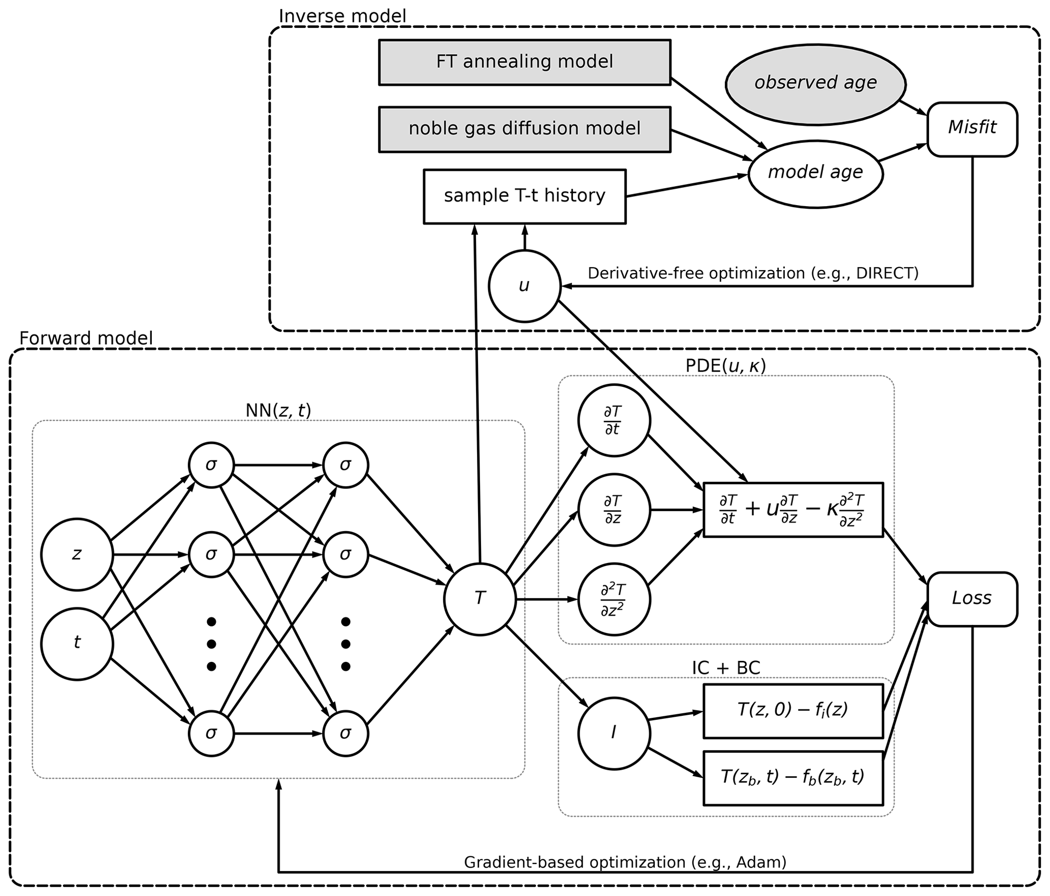
Figure 1Workflow for forward and inverse modelling of the 1D thermal profile for thermochronology. fi and fb are functions for the initial and boundary conditions of the model, respectively.
A key procedure in PINNs is to compute the derivatives of the PDEs. To address this issue, PINNs use automatic differentiation (AD) to represent all differential operators that exist in the PDEs. The AD calculates the derivatives of the outputs with respect to the network inputs based on the chain rule, which is different from numerical computations and avoids discretization and truncation errors. After training with the loss function (and data misfit), the trained network can be used to approximate the solution of PDEs at any location and any time.
PINNs have been applied in various disciplines such as fluid mechanics (Cai et al., 2021a; Raissi et al., 2020; Boster et al., 2023) and have demonstrated great potential in solving governing equations of physical laws in complex domains, especially in solving inverse problems. They have also attracted attention in the community of Earth sciences. For example, Waheed et al. (2021) used PINNs to solve the eikonal equation in 2D for predicting travel times of seismic waves in isotropic and anisotropic media. He and Tartakovsky (2021) used PINNs to solve the advection–dispersion and Darcy flow equations in 1D and 2D fields with spatially varying hydraulic conductivity. Rasht‐Behesht et al. (2022) used PINNs to solve the acoustic wave propagation and full waveform inversions under different and complex boundary conditions.
4.1 Forward solution
4.1.1 Method and problem setup
In our first example, the 1D forward model describes the thermal profile evolution of a 30 km thick crust from 0 to 100 Myr, with the surface and basal temperatures fixed at 0 and 600 °C, respectively. The model exhumation rate remained constant at 0.05 km Myr−1 from 0 to about 60 Myr, after which it increased to 0.6 km Myr−1. The rapid exhumation continued for about 20 million years, and around 80 Myr the exhumation slowed down to 0.1 km Myr−1 and remained at this rate for the rest of the model time (Fig. 2a).
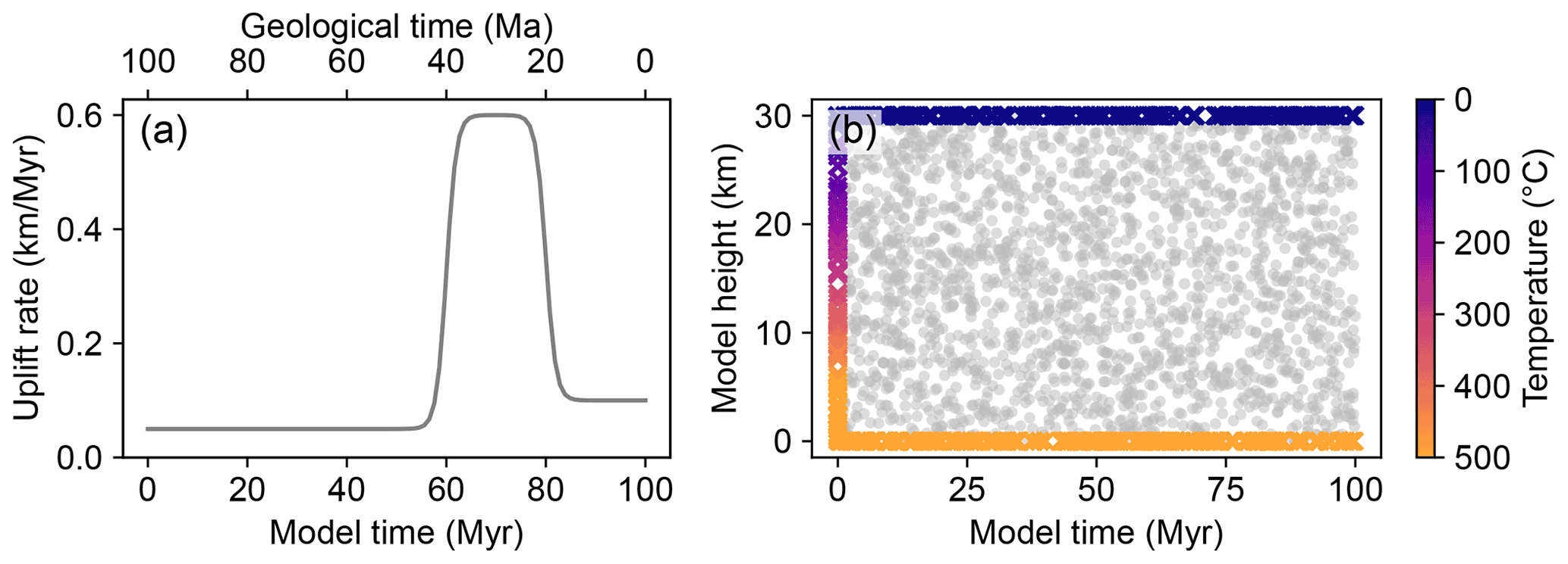
Figure 2Setup of the 1D thermal model of the crust. (a) Rock uplift function of the model. (b) Collocation (grey dots) and boundary condition points (coloured cross) of the PINN model.
The 1D heat advection–diffusion equation to solve is given by
where T is the temperature ( °C), t is the model time (Myr), u is the rock uplift rate (km Myr−1), κ is the thermal diffusivity here set at 25 km2 Myr−1, and z is the vertical position (km) relative to the model base (z= 0). In this model we assume no topographic change over time, so u is equal to the exhumation rate. We solve the model in the space defined by
for which Dirichlet boundary conditions are imposed as
with a linear gradient prescribed for the initial condition, i.e.,
We assume that u is time-dependent and impose its time dependence in terms of logistic functions as
in which u0=0.05 km Myr−1, u1=0.6 km Myr−1, u2=0.1 km Myr−1, t1=60 Myr, t2=80 Myr, and Δt=1 Myr. Δt is an inertia factor that imposes a time length for the transition between two rock uplift rates.
To solve the forward model, we approximate T as a deep neural network (DNN) and such that T(t,z) can be learned by minimizing the loss function
where ℒf penalizes the residual of the governing equations (i.e., PDEs) and ℒb imposes the boundary conditions and initial conditions of the PDEs; α is a weighting parameter. In our experiments presented in the paper, assigning α to 1 ensures effective optimization of the PINN models. Here the initial condition is regarded as a special boundary condition. ℒf and ℒb are computed by
in which f(t,z) is defined for the left-hand side of the heat transfer equation (Eq. 1), depicts the Nf collocation points for f(t,z), and depicts the Nb initial and boundary training data on T(t,z).
In our demonstration, we use the TensorFlow 2 library (Abadi et al., 2016) to build the DNN, which includes three hidden layers with 20 neurons in each layer and an additional transform layer to impose the boundary conditions as hard constraints (Lagaris et al., 1998; Lu et al., 2021). The hyperbolic tangent function (tanh) is used as the activation function, and the Adam optimizer (Kingma and Ba, 2015) is used for minimizing the loss function (Eq. 6). The model is set up with 2000 randomly sampled collocation points. Another 500 points are used to impose the initial and boundary conditions, including 100, 200, and 200 points for the initial thermal structure, the surface temperature, and the basal temperature, respectively (Fig. 2b). For the solution presented here, the DNN is optimized through 50 000 iterations. The initial learning rate is set at 0.001, which decays at a factor of 0.9 for every 1000 steps; i.e., at the ith step the learning rate is .
As a comparison, we also solve the same problem using the finite-element method (FEM), which provides estimates of the heat transfer equations by discretizing the time–space domain using 101 points on the crustal profile and a time step of 1 Myr. To compare the final solutions of the PINN and FEM, we compute the square and infinity norms of the misfits between the predictions of the two methods as
in which and are the temperatures predicted by the PINN and FEM at locations of each element used in FEM and n is the total number of elements. Based on the temperature histories estimated, we also predict the thermochronological ages of the present-day surface rocks using an empirical model of the fission-track annealing (Ketcham et al., 2007) and the noble gas diffusion kinetics (summarized by Reiners and Brandon, 2006) solved by a finite-difference method (Braun et al., 2006). Then the percent errors in ages between the predictions are calculated as
in which apinn and afem are ages calculated by the thermal histories estimated using the PINN and FEM, respectively.
4.1.2 Results
In the first 3000 iterations, the model loss ℒ has decreased rapidly from > 10 000 to < 10 (Fig. 3). After that, the ℒb experiences some fluctuations, but ℒ continues to decrease smoothly and becomes more stable after 30 000 iterations. Figure 4 shows the thermal profiles at different model times predicted by the PINN at various stages of the training, in comparison to the FEM solutions. Between the final PINN and the FEM solutions at model times of 40, 70, and 100 Myr, the l2 calculated for 101 elements is 3.8, 51.0, and 30.0 °C, respectively, and the l∞ is 0.6, 11.4, and 3.5 °C, respectively, indicating reasonable consistency between the two methods (Fig. 4). For the rock at the present-day surface, the PINN also predicts a time–temperature path very consistent with the FEM result (Fig. 5a), with a temperature difference < 20 °C for any point on the path and < 10 °C for the most part of the history (Fig. 5b). For the same rock, the predicted difference in cooling ages between the two modelling methods is < 7 % for apatite (U-Th)/He and apatite fission-track and < 3 % for other thermochronometers (Fig. 5d).
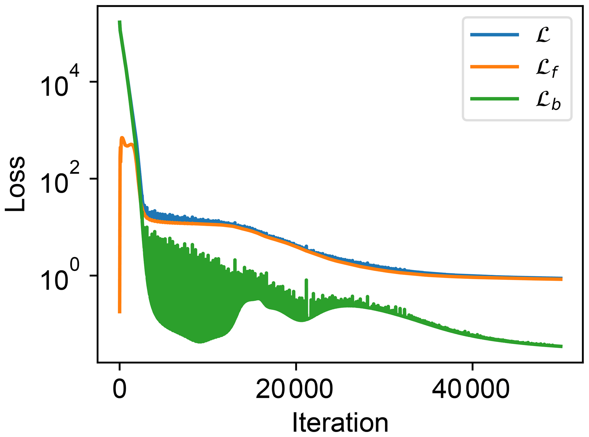
Figure 3Loss curves of the 1D forward model. ℒf and ℒb are losses from the heat transfer equation and the boundary conditions, respectively, whereas ℒ is the total loss.
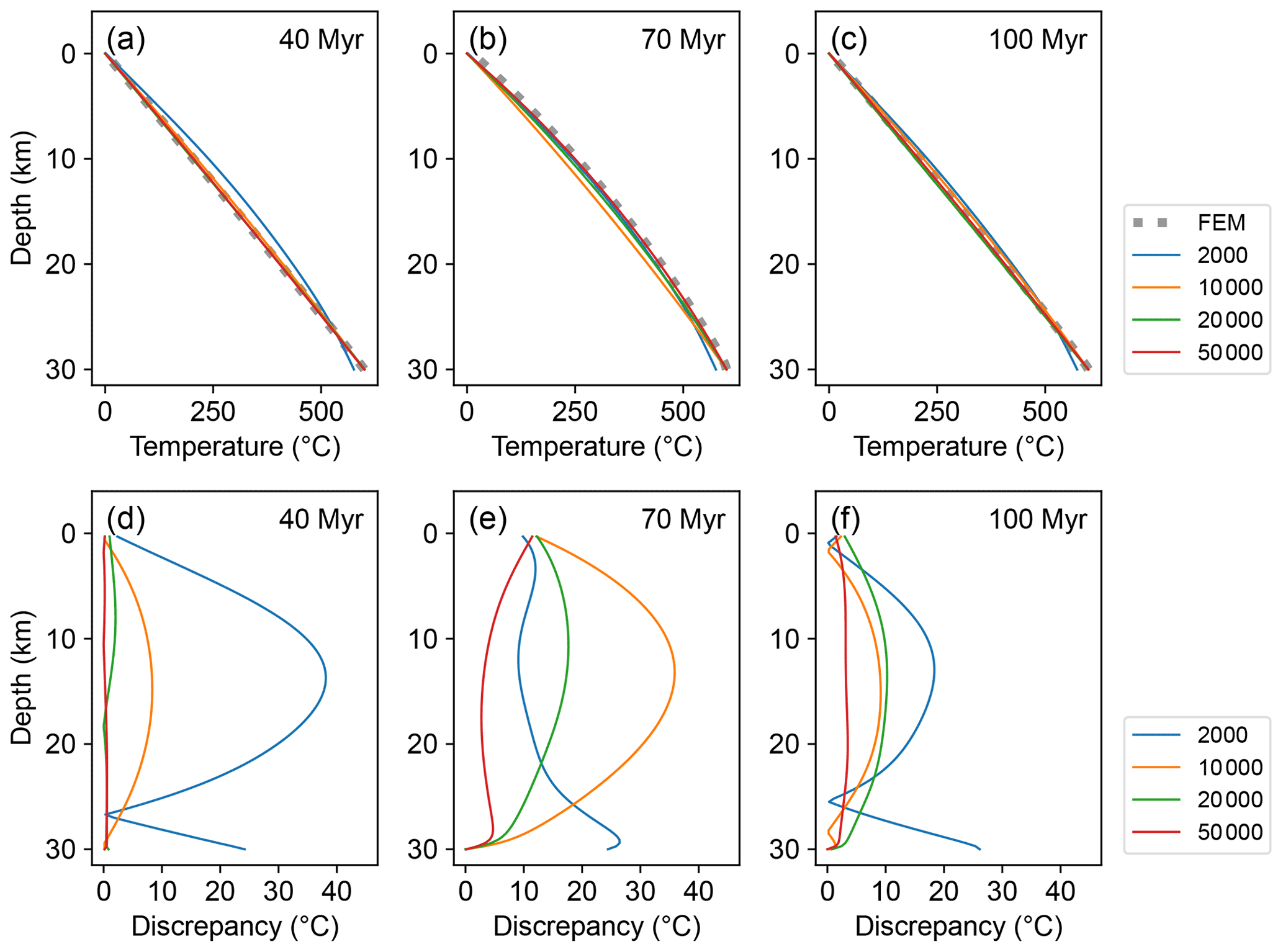
Figure 4Predicted thermal profiles of the crust at different model times. Coloured lines depict the PINN solutions after 2000, 10 000, 20 000, and 50 000 training iterations of training, respectively. The dashed line indicates the solution using the FEM solution.
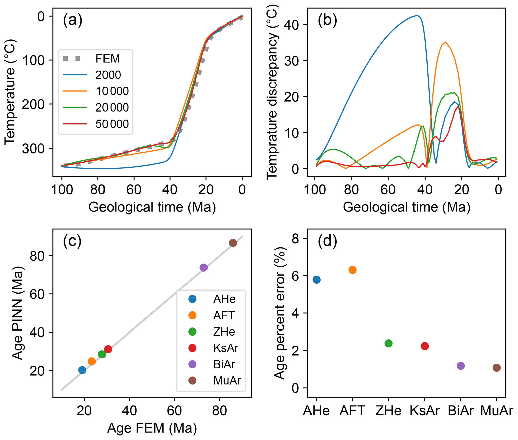
Figure 5Comparison of the thermal histories and ages computed from the PINN and FEM solutions of the forward model. (a) Predicted time–temperature paths and cooling ages for rock sample ended at the surface. Coloured lines represent the PINN predictions after 2000, 10 000, 20 000, and 50 000 iterations, respectively. The dashed line indicates the FEM solution. (b) Temperature discrepancy between the PINN and the FEM solutions. Line colour depicts the iteration numbers performed by the PINN, as shown in the legend of panel (a). (c) Thermochronological ages computed from the thermal models solved by the PINN and FEM. (d) Percent error between the ages predicted by the PINN and FEM. AHe represents apatite (U-Th) He, AFT represents apatite fission track, ZHe represents zircon (U-Th) He, KsAr represents K-feldspar 40Ar 39Ar, BiAr represents biotite 40Ar 39Ar, and MuAr represents muscovite 40Ar 39Ar.
4.2 Inverse problem
4.2.1 Method and model setup
We transform the forward model to an inverse problem by considering u0, u1, u2, t1, and t2 in the rock uplift function (Eq. 5) as unknown parameters. All other parameters defining the thermal model remain the same as in the forward problem (Sect. 4.1). Implementation of the DNN follows a similar setup to that of a forward model, except that the five unknown parameters are updated and optimized during the iterations by reducing the misfit between predicted and observed ages. The age misfit function is defined by
where is the predicted age, is the observed age, is the uncertainty on the observation, and Na is the total number of observed ages. For the problem demonstrated here, synthetic age data predicted from the temperature history computed using the FEM (Fig. 5) are used as data, and a 10 % uncertainty (standard deviation) is assumed for each data point. For calculation of the synthetic observed data, 0.05 km Myr−1, 0.6 km Myr−1, 0.1 km Myr−1, 60 Myr, and 80 Myr are used as “true” values of u0, u1, u2, t1, and t2 in the rock uplift function (Eq. 5), respectively.
The Adam algorithm is used to fit for loss functions derived from the physical law and boundary conditions. To circumvent local minima, the search for optimal values of the unknown parameters in the rock uplift function is conducted using a modified Lipschitzian approach, DIRECT (Jones et al., 1993; Jones and Martins, 2021), which is a global, derivative-free optimization algorithm implemented in the SciPy library (Virtanen et al., 2020). DIRECT operates by progressively partitioning the search space into smaller hyperrectangles and evaluating the objective function at the centre of each. In the subsequent iteration, hyperrectangles with optimal solutions are selected and subdivided for further evaluation. This process is repeated to locate the global minimum in the search space.
The configuration of the DIRECT algorithm requires adjusting a single parameter, ϵ, which defines the minimal acceptable improvement in the function value from the current best solution to the next potentially optimal hyperrectangle for division. A larger ϵ guides the search to explore a broader domain, whereas a smaller ϵ directs a more local exploitation. To optimize the memory usage in our application, we use a strategy in which, after a certain number of iterations, if a parameter value of the optimal solution has no significant change (less than 5 % within the search domain), the DIRECT search recommences within a narrowed search space, reducing the domain for this parameter by 10 %.
More specifically, we define the initial search space for the parameters u0, u1, u2, t1, and t2 within ranges of 0–2 km Myr−1, 0–2 km Myr−1, 0–2 km Myr−1, 0–100 Myr, and 0–100 Myr, respectively. We start the Adam optimization of the DNN model by assigning the midpoint values of the search space to the unknown parameters. After nadam iterations, we use the refined DNN model to explore the space of unknown parameters using the DIRECT approach over ndirect iterations. This process is repeated for multiple cycles to optimize the DNN model and seek the optimum parameter values. In the presented example, the initial nadam is set to 100 and increased by 50 % for each DIRECT cycle, up to a ceiling of 10 000. The learning rate for Adam follows the same schedule used for the forward model; i.e., at the ith iteration the learning rate is . For each cycle, ϵ is maintained at 0.1, and the maximum number of DIRECT iterations, ndirect, is limited to 30 with the maximum number of function evaluated fixed at 1000. Cumulatively, the optimization encompasses > 55 000 Adam iterations and > 290 DIRECT iterations, based on > 15 000 age misfit function evaluations.
We also address the inverse problem using a Markov chain Monte Carlo (MCMC) approach. In the MCMC sampling process, the space of unknown parameters is searched iteratively, and at each iteration the parameter values with higher likelihood are accepted to the Markov chain. After sampling, the chain is used to estimate the probability distribution of the parameters. To evaluate the parameter values, the forward thermal model is simulated with the FEM based on 101 elements on the profile and a time step of 1 Myr. The log-likelihood of a forward model is calculated by comparing the predicted thermochronological ages with the observation, as
In our analysis, the space of five unknown parameters is explored by an affine invariant ensemble sampler (Goodman and Weare, 2010) within predefined domains. The search is conducted by 20 walkers, with each starting from a random location in the parameter space and moving for 50 000 steps. Ultimately, the generated chain comprises 1 000 000 combinations of parameter values from the search space.
4.2.2 Results
The optimization performance is shown as the evolution of the loss from the physical law and boundary conditions (Fig. 6a), as well as misfits between the predicted and observed thermochronological data (Fig. 6b). The loss function curve, despite minor fluctuations between DIRECT cycles (Fig. 6a), shows a reduction pattern similar to that of the forward model (Fig. 3). Figure 7 shows the sampled values used to evaluate the age misfit function. During the DIRECT search, the minimum age misfits decrease progressively until around 200 DIRECT iterations (Fig. 6b), after which the age misfits and parameter values of the optimal solution stabilize (Fig. 7). Finally, the searches of all five parameters are narrowed to ranges centred around the “true” values, except a relatively larger uncertainty on the estimated rate of the rapid uplift, u1.
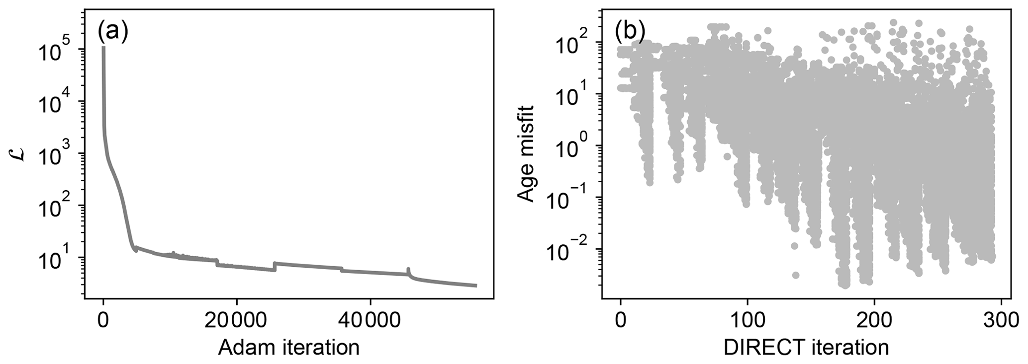
Figure 6Optimization process of the 1D inverse model. (a) Loss function curve of the optimization. (b) Age misfits evaluated by the DIRECT search.
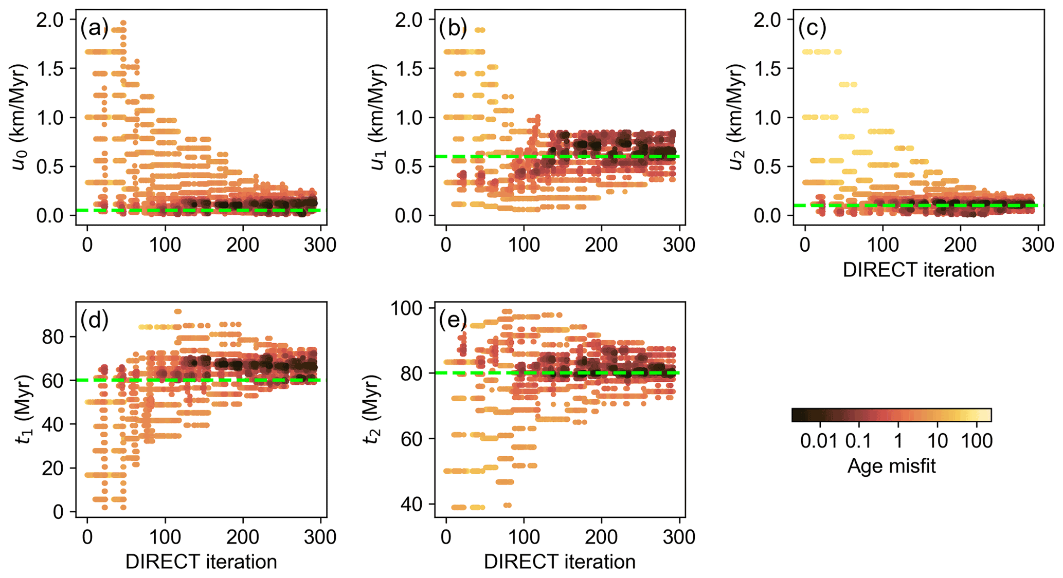
Figure 7Parameter values sampled by the DIRECT method coupled with the PINN model for the 1D inverse model. Dots are colour-coded according to evaluated function value (age misfit). Dashed horizontal lines indicate the “true” parameter values.
The MCMC sampling coupled with the FEM model has also identified optimal values for the unknown parameters. Among the 20 walkers deployed, 3 failed to reach equilibrium at the end of the sampling, whereas the remaining walkers achieved stationary states after around 17 000 iterations (Fig. 8). Similar to the result of the DIRECT search, a large uncertainty exists for the estimate of u1 (Fig. 8b).
Figure 9 presents predictions of the optimized PINN model and the “best-fit” FEM model, the model with the maximum likelihood from the MCMC chain. For both models, the predicted cooling paths of the rock at the current surface align closely with the “true” thermal history (Fig. 9a). The temperature discrepancy at any given time between the PINN solution and the “true” thermal history is < 17 °C and typically < 8 °C (Fig. 9b), whereas that between the “best-fit” FEM model and the “true” thermal history is < 25 °C. Moreover, the optimized PINN and “best-fit” FEM models predict similar thermochronological ages for the surface sample, both consistent with the data computed from the synthetic “true” history (Fig. 9c), with the maximum difference at 5.3 % and 3.7 %, respectively (Fig. 9d).
In this section, we use an example from the Dabie Shan (Fig. 10) to demonstrate the application of PINNs for solving the 3D temperature field under changing topography. Compared to the 1D model, the 3D model requires configuration of more complex boundary conditions and is computationally more intensive. The Dabie Shan in eastern China is a Mesozoic mountain range that underwent rapid exhumation during the Triassic–Jurassic orogeny along the boundary between the North and South China blocks (Nie et al., 1994; Hacker et al., 1995; Ratschbacher et al., 2006). Based on apatite and zircon (U-Th) He and apatite fission-track ages, Reiners et al. (2003) suggested that since the Late Cretaceous, the post-orogenic exhumation of the Dabie Shan has been slow and could be constant at a rate of 0.01–0.06 km Myr−1. By investigating the same dataset using numerical methods, Braun and Robert (2005) estimated the post-orogenic exhumation and topographic evolution of the Dabie Shan and inferred that, since the Late Cretaceous, the mountain range has been exhumed at a mean rate of 0.01–0.04 km Myr−1 and that its topographic relief has reduced by a factor of 2.5–4.5 during the last 60–80 million years. Therefore, thermochronological data provide good constraints on the post-orogenic exhumation of the Dabie Shan, which can be simulated by a simple model with constant exhumation rates, making the mountain range an ideal natural laboratory for testing new thermochronological modelling methods (e.g., Fox et al., 2014).
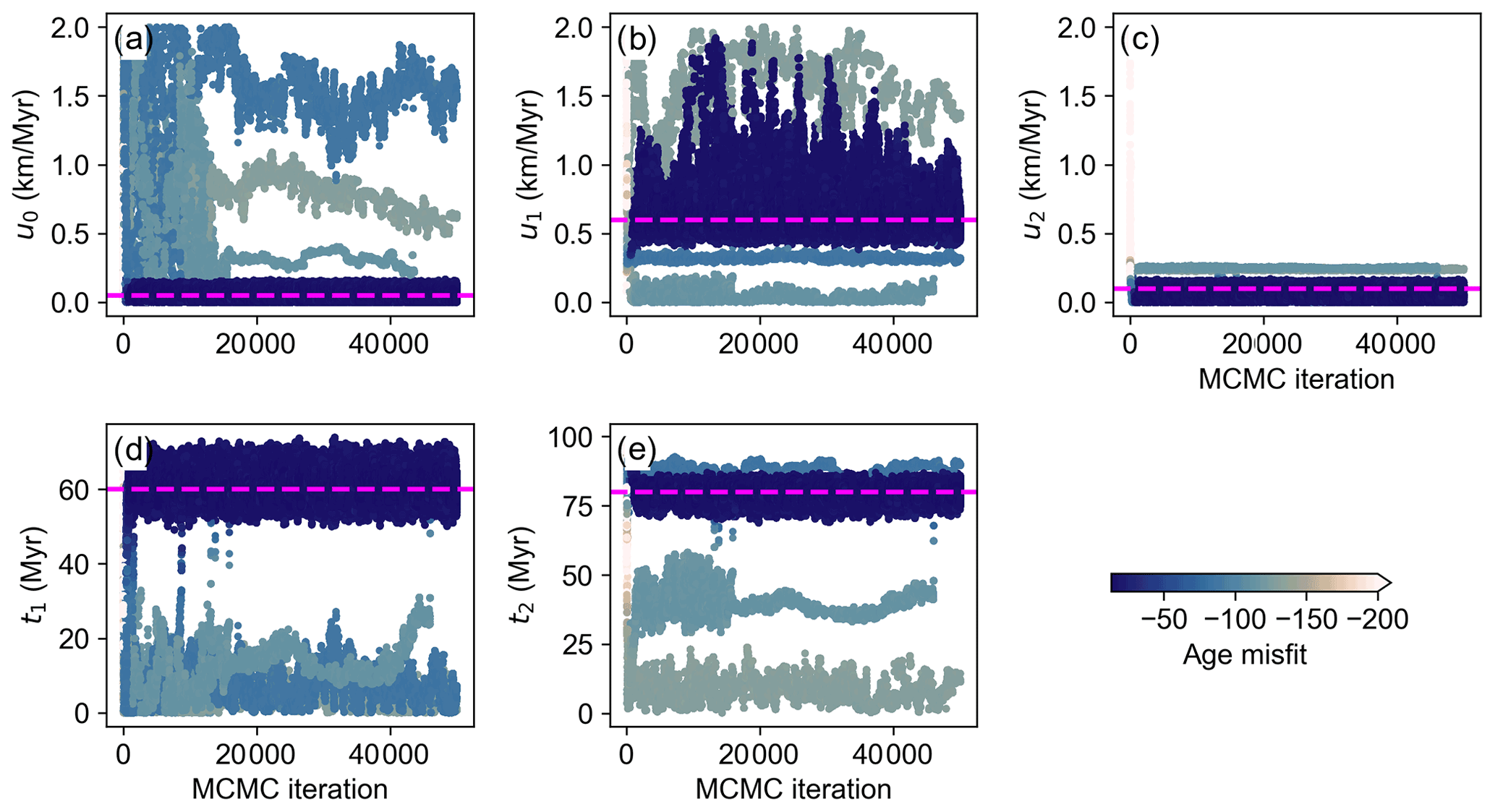
Figure 8Parameter values sampled by the MCMC method coupled with the FEM model for the 1D inverse model. Dots are colour-coded according to the log-likelihood of the forward models. Dashed horizontal lines indicate the “true” parameter values.
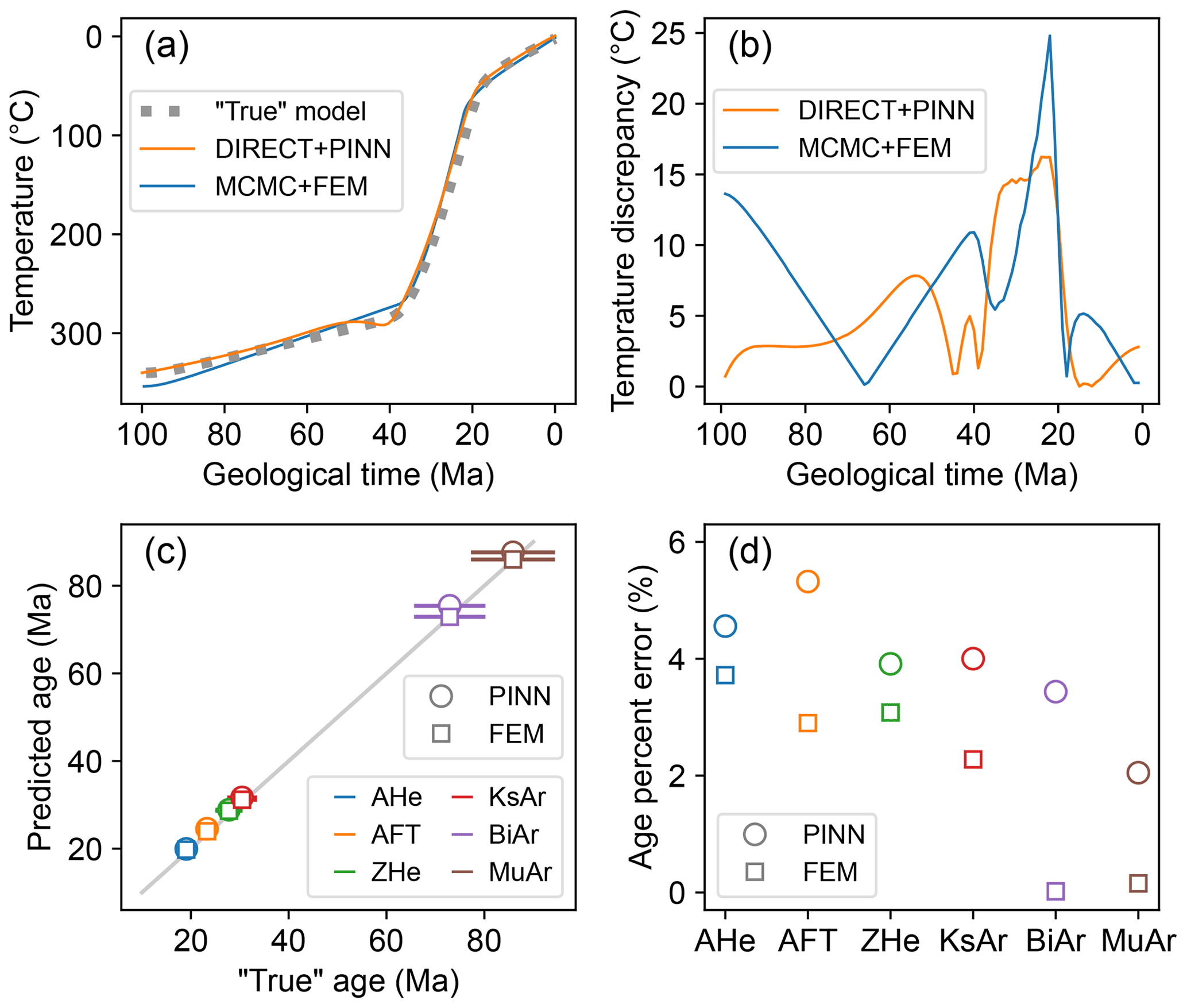
Figure 9Thermal histories and ages predicted by the optimized PINN model and the “best-fit” FEM model from the MCMC sampling chain. (a) Predicted time–temperature paths and cooling ages for a surface rock sample at the end of the model history. (b) Temperature discrepancy between the predicted time–temperature paths and the “true” model. (c) Thermochronological ages calculated from the PINN solution and the “best-fit” FEM model, compared to the synthetic data from the “true” thermal history. (d) Percent error between the predicted ages and synthetic data.
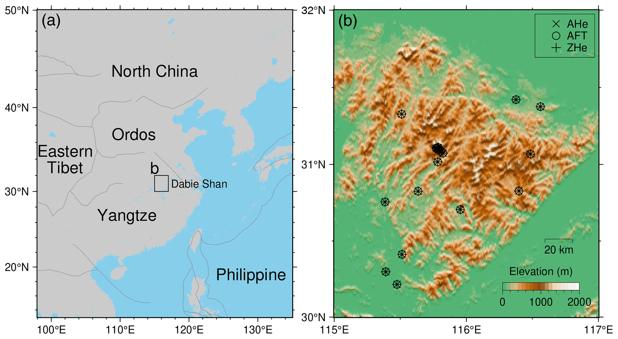
Figure 10(a) Location of the Dabie Shan, eastern China. (b) Topography of the Dabie Shan and locations of thermochronological data.
5.1 Forward solution
5.1.1 Method and model setup
Assuming that the rock motion is in the vertical direction, the 3D heat transfer equation is given by
where x, y, and z are spatial coordinates and other parameters are the same as in Eq. 1. We focus on the last phase of the Mesozoic orogeny and the post-orogenic exhumation history of the mountain and therefore solve its thermal history since 150 Ma. The model space is defined as
in which the range of the z domain is configured to include a crustal thickness (hc=30 km) below sea level and the potential maximum elevation of the mountain range during the model run (hs). The temperature at the base of the model is fixed at 600 °C. The Earth surface temperature is set to 15 °C at sea level and calibrated according to the elevation using an atmospheric lapse rate at −5 °C km−1. Therefore, the boundary conditions are imposed as
in which zs and hs are the vertical coordinate and surface elevation, respectively, with a relationship
To simulate the surface relief change, we follow Braun and Robert (2005) and define a scenario in which between 0 to 70 Myr (equivalent to geological time 150 and 80 Ma) the surface relief was 4 times as high as that of today, and after that the topography has gradually decreased in a linear fashion towards the current level. The topography is imposed as
in which w is a time-dependent amplification factor for topography (Fig. 11b), prescribed by
where w0, set at 4, is the amplification of topography at the beginning of model (t=0) and td, set at 70 Myr, is the model time when the post-orogenic decay of the topography starts. The present-day topography () is extracted from the global elevation model (GEBCO 2014) and resampled to a 2 km resolution.
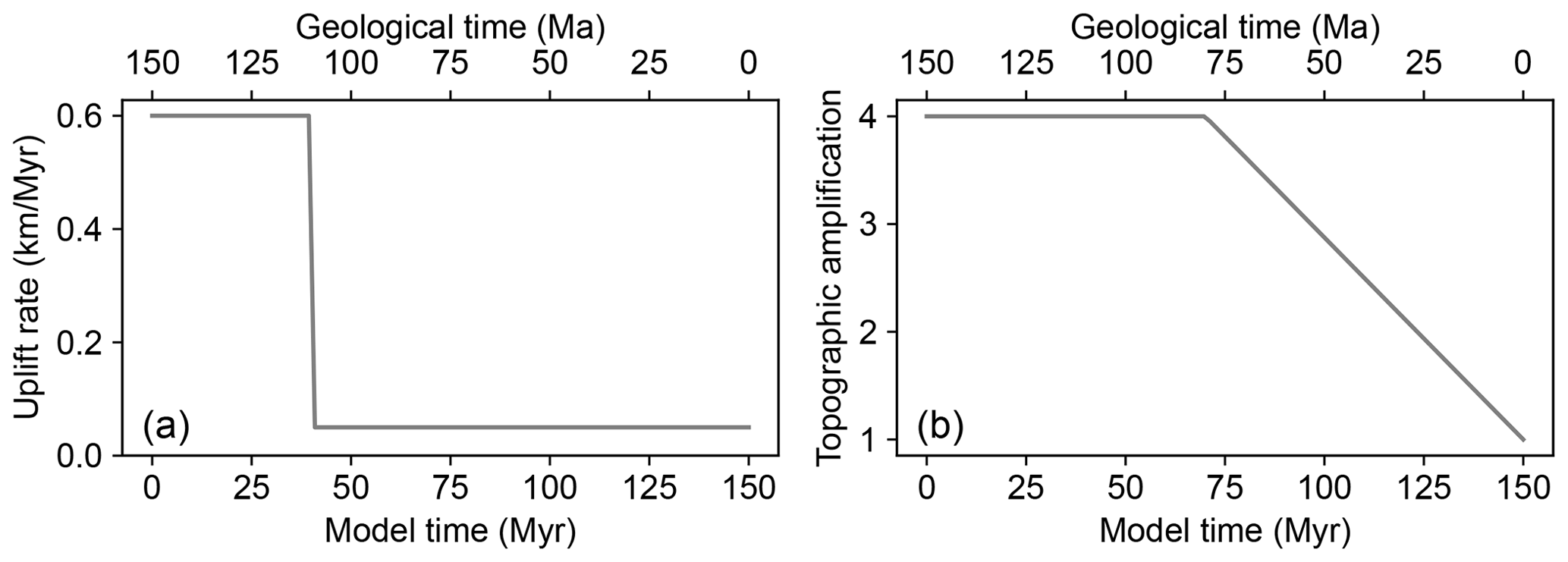
Figure 11Inputs of the 3D thermal evolution model of the Dabie Shan. (a) Rock uplift model. (b) Topographic amplification model.
The initial thermal field is imposed using a linear interpolation of temperatures between the model base and earth surface, i.e.,
Based on conclusions of Reiners et al. (2003) and Braun and Robert (2005), we assume a spatially uniform rock uplift model and define it using a piecewise function (Fig. 11a),
where u0=0.6 km Myr−1, u1=0.05 km Myr−1, and t1=40 Myr. Therefore, the rock uplift remained constant at 0.6 km Myr−1 between 0 and 40 Myr, and then the rate decreased to 0.05 km Myr−1 and remained constant until the end of model.
Similarly to the solution of the 1D model, we approximate T as a DNN and train it using the same loss function (Eq. 6). The loss functions from 3D heat transfer law and boundary (and initial) conditions become
in which stands for the left-hand side of the 3D heat transfer equation (Eq. 14).
The DNN used for the 3D model comprises 16 hidden layers, each with 20 neurons, and an additional layer to transform the outputs. The tanh activation function and Adam optimizer are employed, similarly to those used for the 1D model. An exponential decay function, , is used to define the learning rate. We selected 2000 random points to define the initial thermal field (Fig. 12a), and we used 2000 and 10 000 points to impose the temperatures at the model base and on the surface topography, respectively (Fig. 12b). We configured the model with 100 000 collocation points (Fig. 12c), half of which are allocated randomly within the orogenic phase () and the remainder during the post-orogenic phase ().
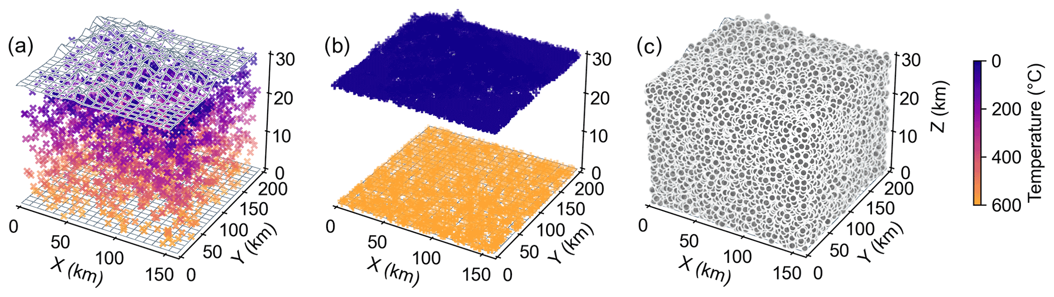
Figure 12The initial and boundary conditions and collocation points for the 3D thermal model of the Dabie Shan. Control points are projected onto the space. (a) The initial thermal field. (b) Boundary temperatures at the surface and base of the model. (c) Collocation points.
To evaluate the accuracy of the solution of the PINN, we also computed the thermal field evolution of the Dabie Shan using the FEM code, Pecube (Braun, 2003). The FEM model is set up on a () grid, with the thermal field solved at a time step of 1 Myr. The rock uplift history and boundary conditions are identical to those in the PINN model.
5.1.2 Results
Figure 13 shows the loss curves through the optimization process, which present a progressive decrease until stabilization after approximately 300 000 iterations. Figure 14 presents the temperature profiles on three transects across the model at 40 and 150 Myr computed by the PINN, which reveal significant perturbations of the crustal thermal structures caused by the rock uplift and surface topography, resembling the patterns of the FEM solution. At 40 Myr, at the majority of locations (90 %), the temperature differences predicted by the PINN and FEM are < 10 °C. On these transects, the l2 and l∞ of the temperature discrepancies between the solutions of the two methods are 240–426 and 26–35 °C, respectively; these values are calculated from the solutions at the 3131 element locations used in the FEM (Fig. 15). At 150 Myr when the rock uplift rate has decreased and the topographic relief is lower, the discrepancies between the PINN and FEM solutions are significantly reduced, with the l2 and l∞ decreasing to 70–112 and 8–10 °C, respectively.
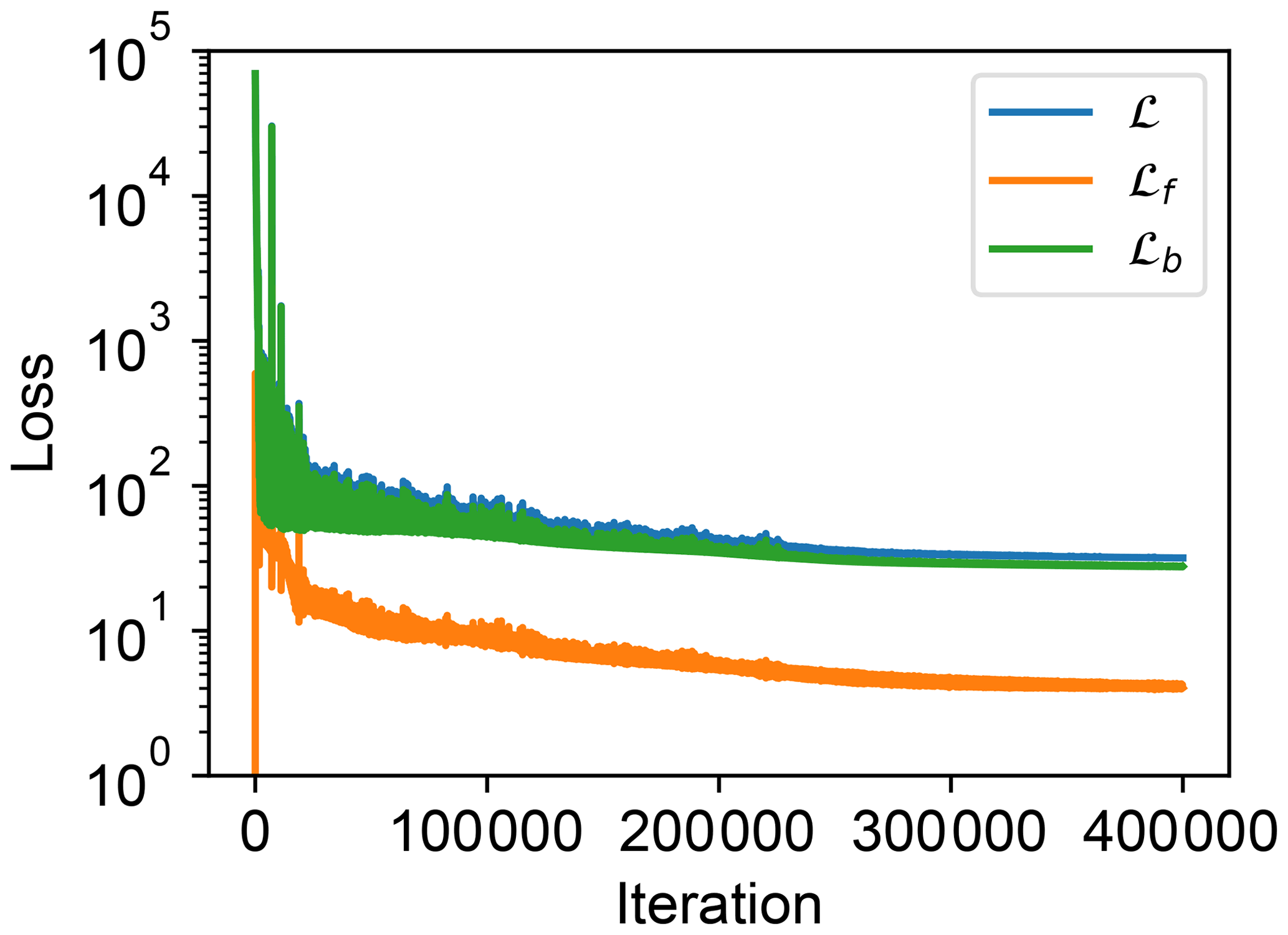
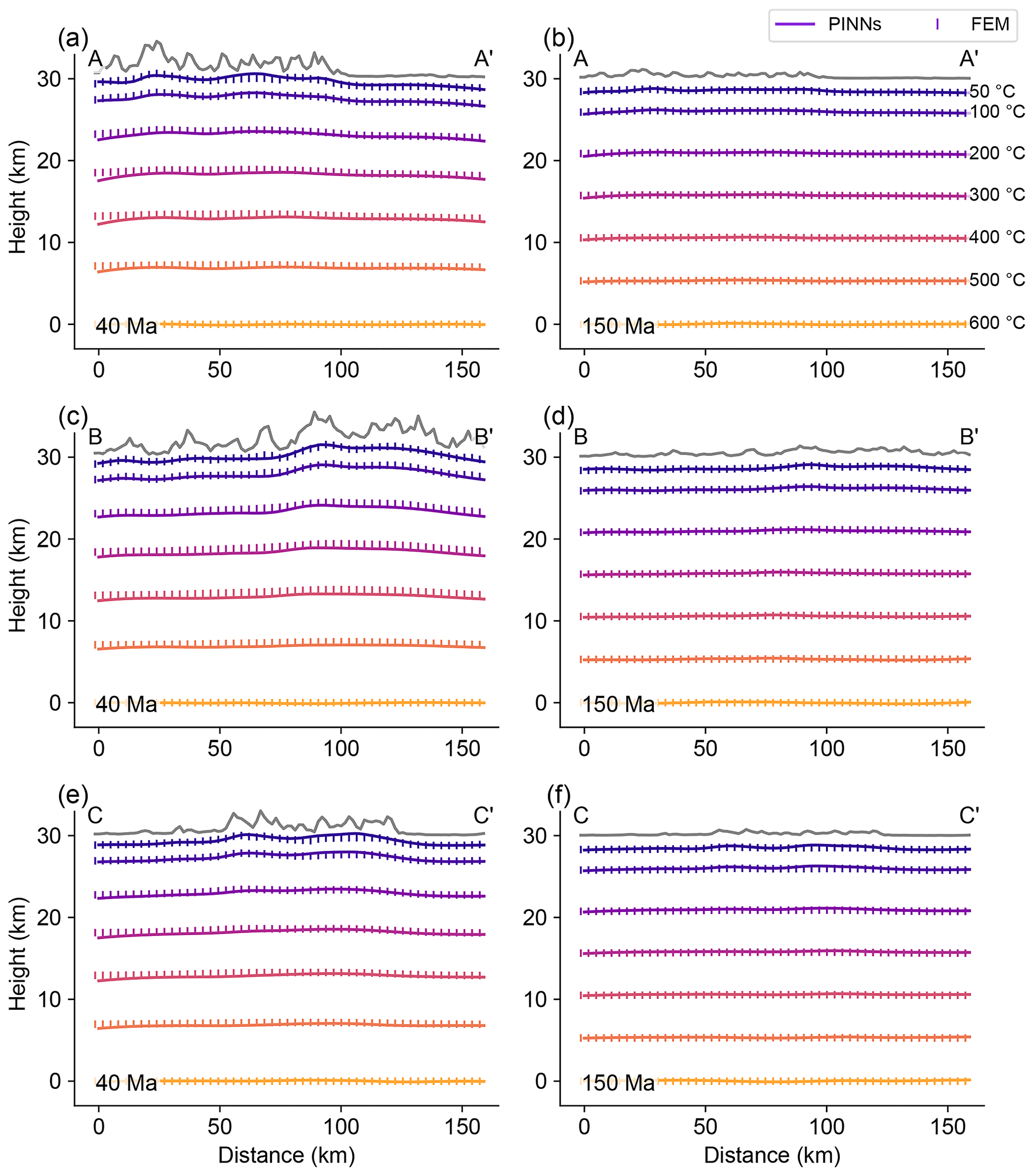
Figure 14Predicted isotherms on three transects across the Dabie Shan at model times of 40 and 150 Myr. Solutions using the PINN and FEM are compared. Locations of the transects are shown in Fig. 16.
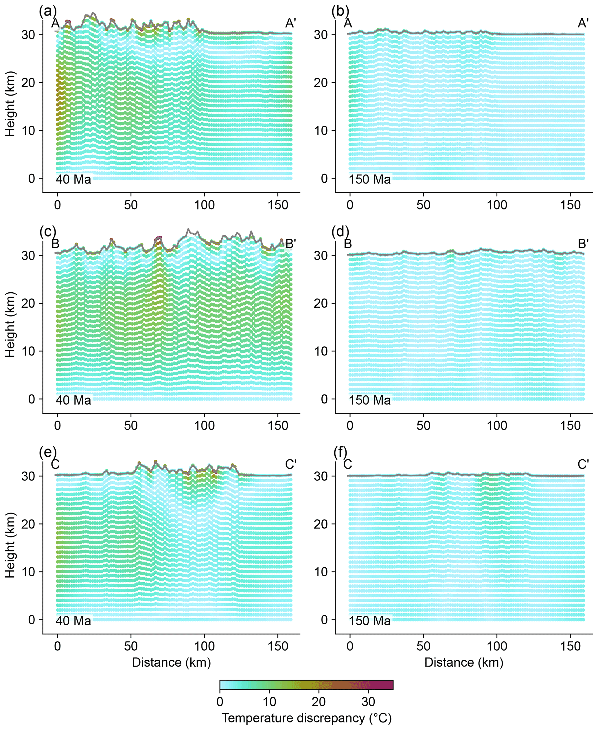
Figure 15Discrepancies in temperature solutions between the PINN and FEM on three transects across the Dabie Shan at model times of 40 and 150 Myr. Locations of the transects are shown in Fig. 16.
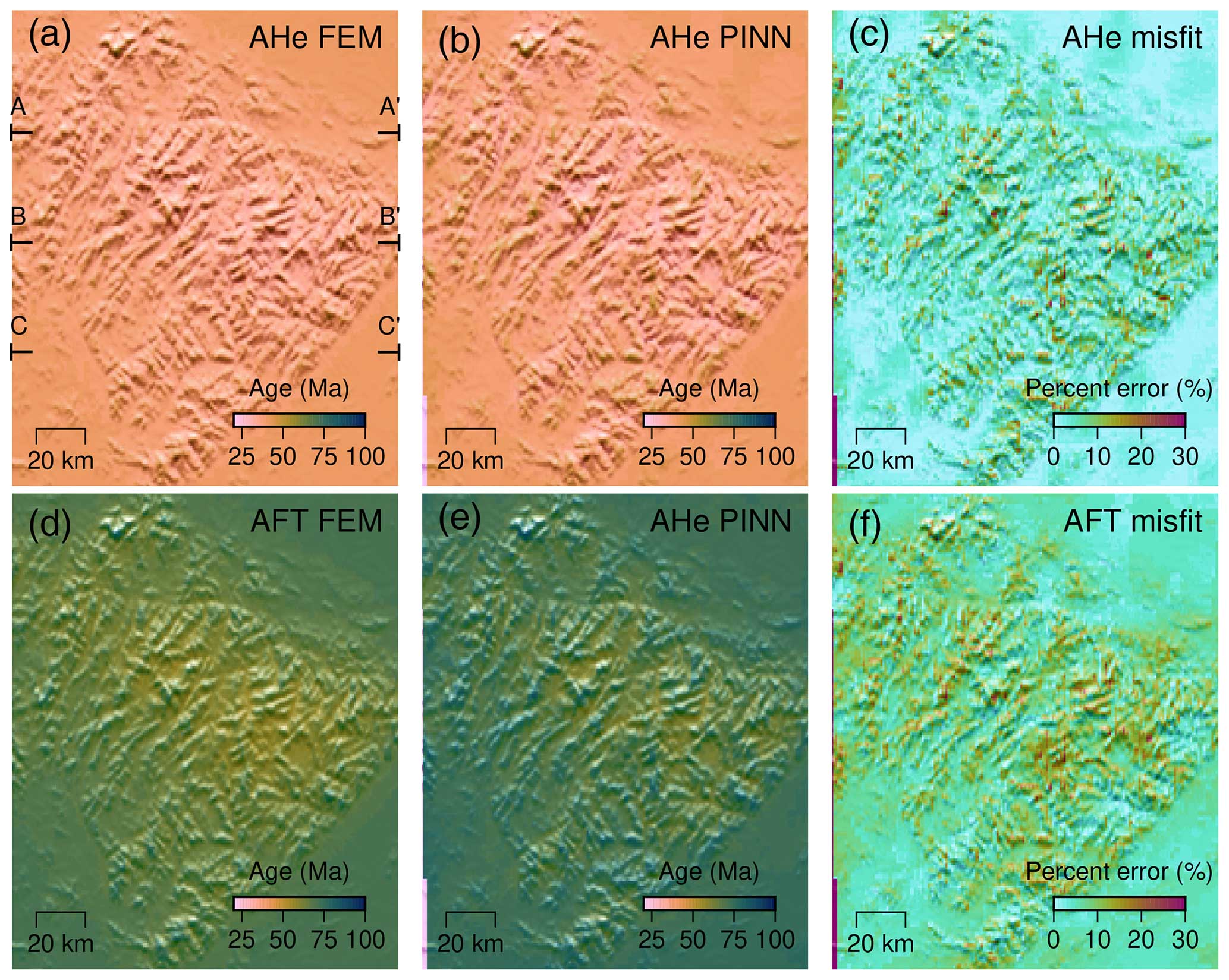
Figure 16Maps of the Dabie Shan showing the predicted age misfits between the PINN and FEM solutions. A–A′, B–B′, and C–C′ indicate locations of the transects in Fig. 14.
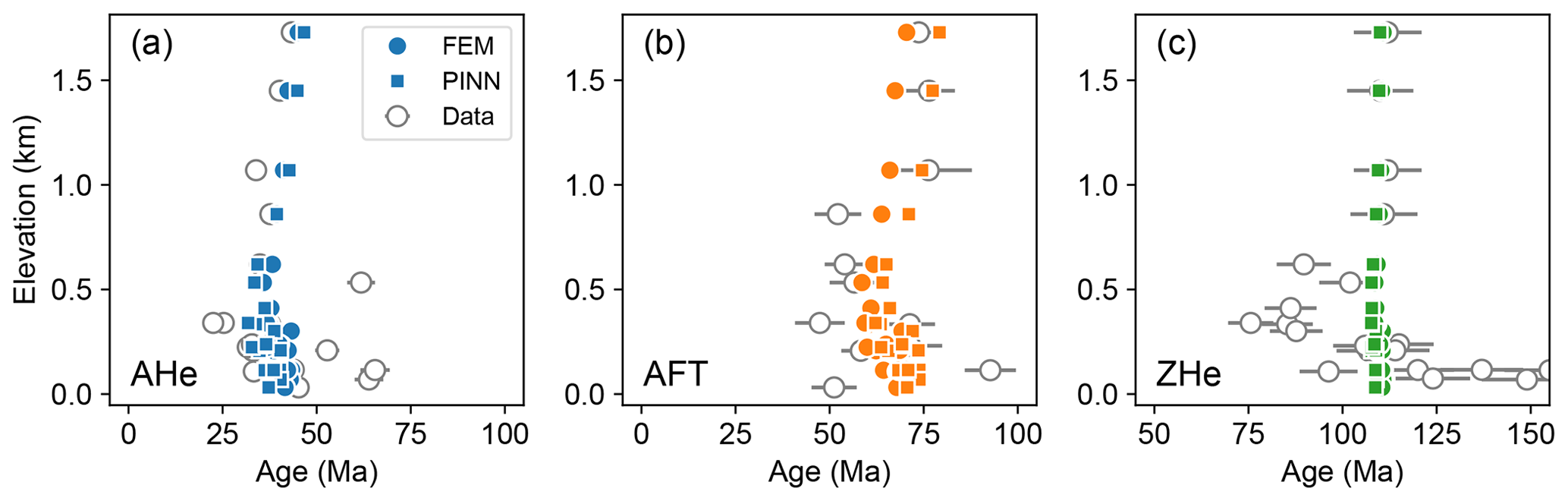
Figure 16 shows the misfits in the AHe and AFT ages for the present-day surface rocks at 42 000 locations, which are calculated from their thermal histories predicted by the PINN and FEM. For both thermochronometers, the predicted age misfits at all locations are < 20 %. At most locations (90 %), the misfits between AHe ages predicted by the two methods are < 6 %, and those between AFT ages are < 10 %. Compared to AHe ages, the higher misfits in predicted AFT ages reflect larger discrepancies in the temperature solutions between the PINN and FEM for the periods of high rock uplift rate and significant topographic relief (Fig. 15). At the sites with observed data, the misfits in predicted AHe, AFT, and ZHe ages between the PINN and FEM solutions are < 13 %, < 15 %, and < 2 %, respectively, which generally fall within the error margins or clustering ranges of the measured data (Fig. 17).
5.2 Inverse problem
5.2.1 Model setup
To test the effectiveness of PINNs in constraining the exhumation models using real data, we formulate an inverse problem, aiming to estimate the post-orogenic uplift and topographic evolution of the Dabie Shan using published low-temperature thermochronological ages. In our analysis, we seek to constrain the orogenic rock uplift rate (u0), the ending time of the rapid uplift (t1), and the rock uplift rate during the post-orogenic period (u1), as described in Eq. (21). In addition, we estimate the amplification factor for the topography during the orogenic phase (w0) and the onset time for topographic decay (td) as described in Eq. (19). We confine the search for these five parameters, u0, u1, w0, t1, and td, within the ranges of 0–1 km Myr−1, 0–1 km Myr−1, 0–6, 0–50 Myr, and 50–100 Myr, respectively. To guide the optimization process, thermochronological age data reported by Reiners et al. (2003) (Fig. 10b) are used, considering only the ages < 150 Ma.
Similarly to the 1D model inversion, we use both the Adam and DIRECT algorithms to optimize the DNN model and explore the search space. For the Adam iterations, we set the learning rate using the same exponential decay function applied in the forward 3D model. In the DIRECT search, we use the “restart-and-zoom-in” strategy akin to that employed in the forward 3D model but increase the number of cycles to 40. Each DIRECT cycle includes up to 30 iterations and a maximum of 1000 function evaluations. Altogether, the inversion process comprises > 500 000 Adam iterations and > 1000 DIRECT iterations, evaluating > 40 000 age misfit functions.
As a reference, we also explore the multi-dimensional parameter space using the neighbourhood algorithm (NA) (Sambridge, 1999a), in which the forward model is computed using Pecube (Braun, 2003). It is worth noting that, compared to the modelling employed by Braun and Robert (2005) in the same region, we do not consider the isostatic rebound in response to the exhumation; thus the result may differ slightly. To reduce the computational demands compared to the model used in the forward problem (Sect. 5.1), we reduce the FEM grid size to by increasing the horizontal spacing between elements. The NA divides the parameter space into Voronoi cells and evaluates the model misfit according to the parameter values at the cell centres. The subsequent iteration generates new samples within a subset of cells containing the best-fit models from the previous iteration. This process is repeated to find the optimal parameter values that fit the observed data. Here the NA search for parameters u0, u1, w0, t1, and td are within the same domains as predefined for the inversion of the PINN model. The search comprises 150 iterations with each running forward models in 60 cells, out of which the 75 % best cells are resampled for the next iteration. In total, the NA inversion includes 9060 forward Pecube runs.
5.2.2 Results
The training process of the PINN is shown in Fig. 18 as the evolution of the thermal model loss and the misfits in predicted ages. The parameter values evaluated by the DIRECT search are shown in Fig. 19. Notably, the loss function curve displays more fluctuation compared to the forward model, but it maintains a general decreasing trend. This fluctuation reduces as the learning rate decreases (Fig. 18a). Upon the stabilization of the loss function after approximately 200 000 Adam and 500 DIRECT iterations, the predicted minimum age misfits have a declining pattern for around 250 DIRECT iterations and show minimal changes thereafter (Fig. 18b). During the parameter search, convergence mostly occurs within the initial 100 and then from 500 to 1000 DIRECT iterations (Fig. 19). Finally, estimates for the parameters u0, u1, w0 , t1, and td are confined to the ranges of 0.7–0.95 km Myr−1, 0–0.18 km Myr−1, 2–5.5, 21–45 Myr, and 74–91 Myr, respectively.
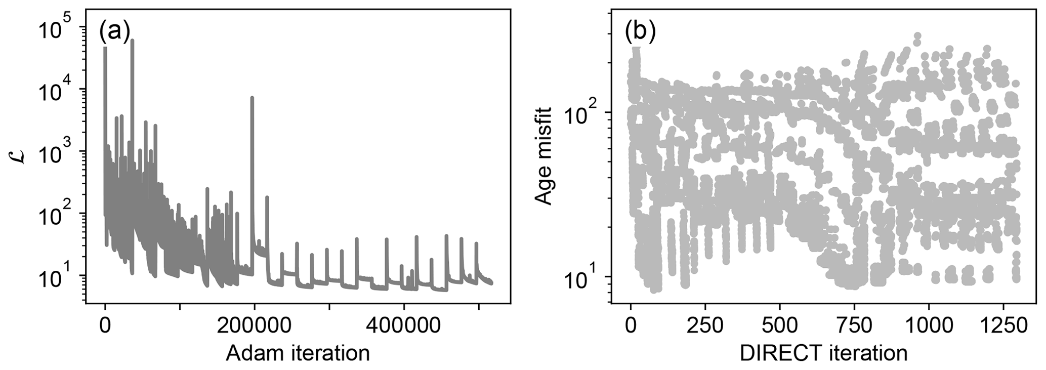
Figure 18Optimization process of the 3D inverse model of the Dabie Shan. (a) Loss function curve of the optimization. (b) Age misfits evaluated by the DIRECT search.
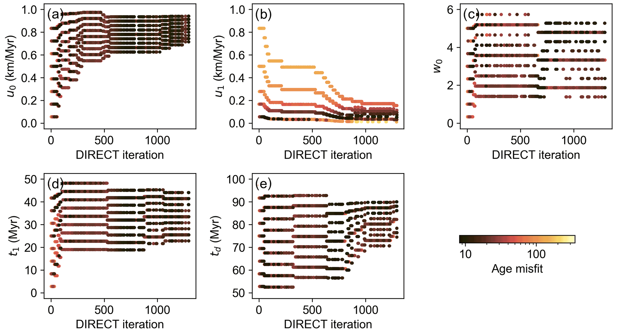
Figure 19Evaluated parameter values for the 3D inverse model of the Dabie Shan using the DIRECT algorithm (Jones et al., 1993) and the PINN model.
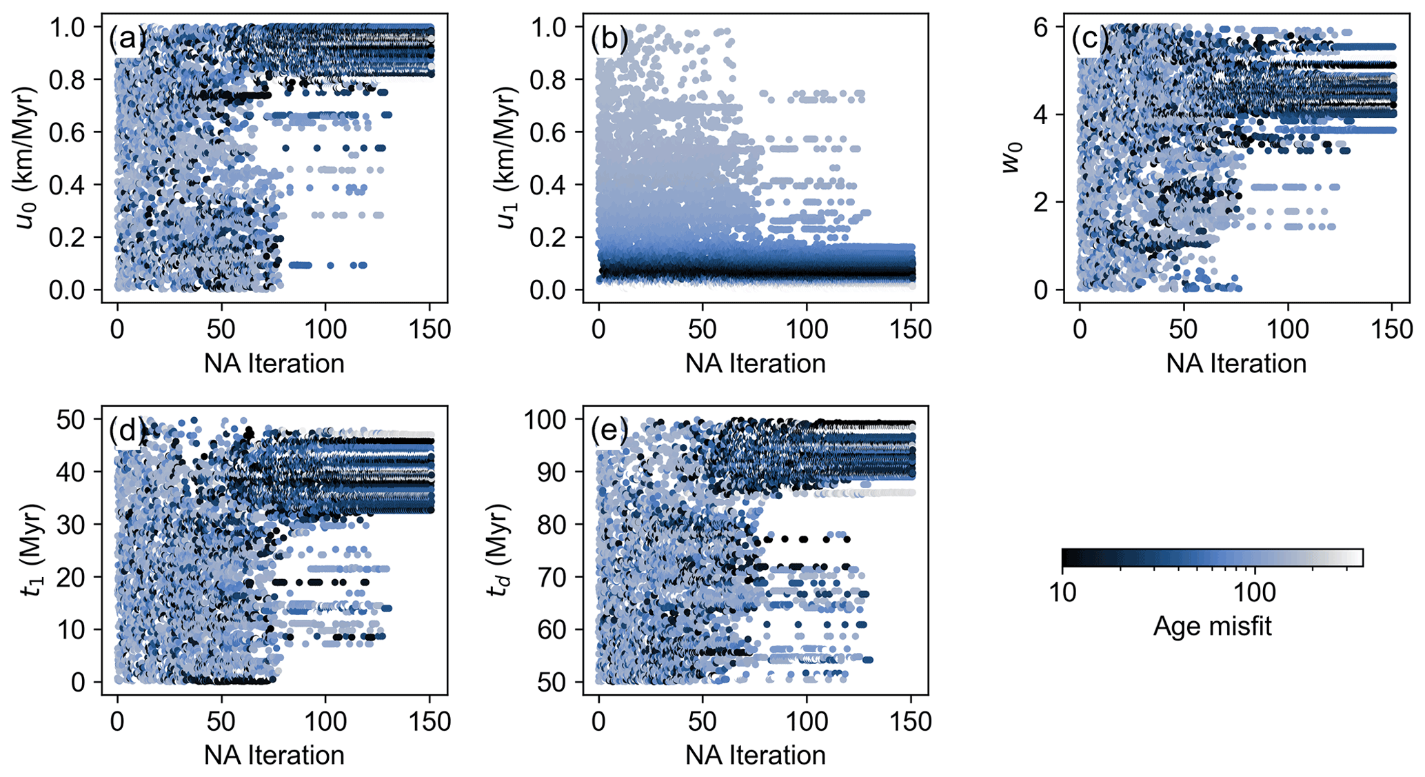
The NA search based on forward Pecube models exhibits patterns comparable to those observed in the optimization of the PINN model. Specifically, the search for u0 also converges rapidly to a range of 0–0.1 km Myr−1, while the other four sampled parameters show significant convergence only after approximately 80 iterations. In the NA search the parameters u0, u1, w0, t1, and td are ultimately confined within the ranges of 0.8–1 km Myr−1, 0.01–0.13 km Myr−1, 4.1–5.1, 33–44 Myr, and 88–97 Myr, respectively (Fig. 20). Except for the parameter w0 being confined to a narrower range by the NA, the search results by the two inverse models overlap over significant ranges.
6.1 Comparison between the PINN and numerical method
We have demonstrated that, in the study of thermochronology, PINNs are comparably as effective as conventional numerical methods. In both the 1D and 3D forward models we presented, the mean temperature difference across all points at any given time between the PINN and FEM solutions is < 0.5 °C, with the maximum difference at specific points ranging between 10 and 30 °C, which appear to occur during periods of rapid rock uplift and exhumation (Figs. 5b and 15). This level of discrepancy is minor compared to the typical uncertainties in thermal histories derived from thermochronological data. For 90 % of the surface samples in our examples, temperature discrepancies between the PINN and FEM solutions resulted in < 10 % misfits in the predicted ages. Larger misfits up to 20 % were found in cooling ages of samples that record rapid rock exhumation in areas with high topographic relief (Figs. 10b and 17b). These misfits in age estimates are at comparable magnitude to inherent uncertainties in measured age data, and they can be less significant than the data dispersion caused by the variability in the kinetics of noble gas diffusion or fission-track annealing.
For simple forward models, conventional numerical methods do not require optimization, thus having an advantage in the computational efficiency over PINNs. For instance, solving the 1D forward model in Sect. 4.1 using the FEM required a few milliseconds on a modern CPU (Intel Xeon Gold 5420+), whereas training the PINN model with 80 neurons for 50 000 iterations on a GPU (NVIDIA RTX 6000 Ada) took several hundred seconds, which is 5 orders of magnitude longer than the time required for the FEM solution. This contrast diminishes as the model's dimensionality, size, and complexity increase. To illustrate this, simulating the 3D forward model of the Dabie Shan in Sect. 5.1 on a grid over 150 time steps took approximately 2400 s using Pecube, whereas training the PINN with 320 neurons over 400 000 iterations required around 32 000 s, merely 1 order of magnitude longer than the FEM solution.
For inverse problems, the computational time escalates as the parameter space expands, which necessitates the evaluation of a larger number of numerical models. In Sect. 4.2, the MCMC sampling which required the evaluation of 1 000 000 FEM models consumed approximately 8000 s. This duration represents an increase by 6 orders of magnitude from a single forward solution. In contrast, the inverse analysis using DIRECT and the PINN model, which evaluated over 15 000 age misfit functions, was completed within 7000 s, marking an increase in time by only 1 order of magnitude from the PINN forward model solution. For the 3D Dabie Shan model (Sect. 5.2), the NA inversion, using 30 CPU cores and coupled with a Pecube model on an grid, required approximately 300 000 s of clock time to explore the search space and evaluate 9060 misfit functions. The cumulative computation time across all processors amounted to ∼ 9 000 000 s, which is 4 orders of magnitude greater than the time used for solving a single forward model. Conversely, the DIRECT search and the PINN model optimization evaluated 38 130 age misfit functions within 560 000 s, which is increased by 1 order of magnitude from the 3D forward model.
Although the computational performance metrics presented herein are not derived from rigorous benchmarks, they provide a preliminary comparison of the efficiency of PINNs and traditional numerical methods. It is evident that, for inverse problems, PINNs have an advantage due to their seamless integration of parameter search and forward model optimization within one single training process. This integration prevents PINNs from an exponential increase in computational time as the dimensionality of the inverse problem increases, illustrating the method's potential for inverse analysis of expansive models with complex boundary conditions, which can be unattainable with traditional numerical methods.
6.2 Directions for future development
In our applications, we have modelled the rock uplift as a vector in the vertical direction independent of spatial locations. However, thermo-tectonic research often requires us to consider rock uplift and exhumation rates that vary both temporally and spatially. Previous work (e.g., Cai et al., 2021b) has demonstrated the feasibility of incorporating a comprehensive 3D velocity field in the DNN. However, the effectiveness of PINNs in scenarios with abrupt changes in the velocity field requires further exploration or improvement (e.g., Rasht‐Behesht et al., 2022). This capability is vital for studying tectonically active regions, where fault activities can significantly disrupt exhumation and geothermal patterns, and thus will be a focus of our future development of the method.
Our current approach to the inverse problem yields an optimized solution of the heat transfer model. Although the search process results in a collection of sampled parameter values, they are not appraised to quantify the uncertainties associated with the optimized model. To address this, a Bayesian neural network can be employed in the PINN framework. This way, the parameters in the neural network would follow Gaussian distributions in contrast to the deterministic parameters of a traditional fully connected network (Yang et al., 2021). This modification would allow the Bayesian PINNs to accommodate noisy data and provide uncertainty estimates for the inferred parameters in the PDEs.
We have outlined the basic configurations for optimizing PINNs and their integration with the DIRECT search algorithm for inverse analysis. However, we expect that model domains of greater complexity, which require a denser array of collocation points, may need more fine-tuning of the training strategies. Enhancing the algorithm and its configuration for the efficient optimization of PINNs is an active field of research (Jagtap et al., 2020; Shukla et al., 2021). For the inverse analysis, the flexibility in problem formulation with PINNs facilitates the incorporation of various search and optimization algorithms. Our ongoing efforts include integrating and testing these algorithms, to ensure stable training outcomes from PINNs.
We have presented applications of physics-informed neural networks (PINNs) in solving crustal heat transfer problems for thermochronology. By harnessing the computational power of deep learning, PINNs offer a flexible and efficient alternative to traditional analytical and numerical techniques. The method allows a straightforward integration of initial and boundary conditions, as well as observed data, and can be used together with gradient-based and derivative-free optimization methods to solve both forward and inverse problems. By applying PINNs to a 1D synthetic model and a 3D natural model of the Dabie Shan under varying tectonic and topographic conditions, we have demonstrated the potential of this approach for estimating the thermal and exhumation histories of the crust during tectonic and landscape evolution. Future work will focus on improving the optimization strategies for inverse models, quantifying the model uncertainties, and expanding the application of PINNs to more intricate geomorphic, geologic, and geodynamic scenarios.
Codes for examples shown in the paper, implemented using the TensorFlow 2 library, are available at https://doi.org/10.5281/zenodo.11454363 (Jiao, 2024).
Apatite and zircon (U-Th) He and apatite fission-track ages from the Dabie Shan were published by Reiners et al. (2003).
RJ conceived the idea, developed the code, and carried out the tests. SC tested the codes. All authors wrote the paper together.
The contact author has declared that none of the authors has any competing interests.
Publisher’s note: Copernicus Publications remains neutral with regard to jurisdictional claims made in the text, published maps, institutional affiliations, or any other geographical representation in this paper. While Copernicus Publications makes every effort to include appropriate place names, the final responsibility lies with the authors.
We thank Stan Dosso for his feedback on the paper.
Ruohong Jiao's research is supported by the Natural Sciences and Engineering Research Council of Canada (Discovery Grant 2019-04405).
This paper was edited by Brenhin Keller and reviewed by David Whipp and Kendra Murray.
Abadi, M., Agarwal, A., Barham, P., Brevdo, E., Chen, Z., Citro, C., Corrado, G. S., Davis, A., Dean, J., Devin, M., Ghemawat, S., Goodfellow, I., Harp, A., Irving, G., Isard, M., Jia, Y., Jozefowicz, R., Kaiser, L., Kudlur, M., Levenberg, J., Mané, D., Monga, R., Moore, S., Murray, D., Olah, C., Schuster, M., Shlens, J., Steiner, B., Sutskever, I., Talwar, K., Tucker, P., Vanhoucke, V., Vasudevan, V., Viégas, F., Vinyals, O., Warden, P., Wattenberg, M., Wicke, M., Yu, Y., and Zheng, X.: TensorFlow: large-scale machine learning on heterogeneous systems, arXiv [preprint], https://doi.org/10.48550/arXiv.1603.04467, 16 March 2016. a, b
Boster, K. A., Cai, S., Ladrón-de Guevara, A., Sun, J., Zheng, X., Du, T., Thomas, J. H., Nedergaard, M., Karniadakis, G. E., and Kelley, D. H.: Artificial intelligence velocimetry reveals in vivo flow rates, pressure gradients, and shear stresses in murine perivascular flows, P. Natl. Acad. Sci. USA, 120, e2217744120, https://doi.org/10.1073/pnas.2217744120, 2023. a
Brandon, M. T., Roden-Tice, M. K., and Carver, J. I.: Late Cenozoic exhumation of the Cascadia accretionary wedge in the Olympic Mountains, northwest Washington State, Bull. Geol. Soc. Am., 110, 985–1009, https://doi.org/10.1130/0016-7606(1998)110<0985:LCEOTC>2.3.CO;2, 1998. a, b, c
Braun, J.: Pecube: a new finite-element code to solve the 3D heat transport equation including the effects of a time-varying, finite amplitude surface topography, Comput. Geosci., 29, 787–794, https://doi.org/10.1016/S0098-3004(03)00052-9, 2003. a, b, c, d, e
Braun, J. and Robert, X.: Constraints on the rate of post-orogenic erosional decay from low-temperature thermochronological data: Application to the Dabie Shan, China, Earth Surf. Proc. Land., 30, 1203–1225, https://doi.org/10.1002/esp.1271, 2005. a, b, c, d
Braun, J., Beek, P. V. D., and Batt, G.: Quantitative thermochronology: numerical methods for the interpretation of thermochronological data, Cambridge University Press, 1st Edn., ISBN 978-0-521-83057-7, 978-0-511-61643-3, 978-1-107-40715-2, https://doi.org/10.1017/CBO9780511616433, 2006. a
Braun, J., van der Beek, P., Valla, P., Robert, X., Herman, F., Glotzbach, C., Pedersen, V., Perry, C., Simon-Labric, T., and Prigent, C.: Quantifying rates of landscape evolution and tectonic processes by thermochronology and numerical modeling of crustal heat transport using PECUBE, Tectonophysics, 524-525, 1–28, https://doi.org/10.1016/j.tecto.2011.12.035, 2012. a, b
Cai, S., Mao, Z., Wang, Z., Yin, M., and Karniadakis, G. E.: Physics-informed neural networks (PINNs) for fluid mechanics: A review, Acta Mech. Sinica, 37, 1727–1738, 2021a. a
Cai, S., Wang, Z., Fuest, F., Jeon, Y. J., Gray, C., and Karniadakis, G. E.: Flow over an espresso cup: inferring 3-D velocity and pressure fields from tomographic background oriented Schlieren via physics-informed neural networks, J. Fluid Mech., 915, A102, https://doi.org/10.1017/jfm.2021.135, 2021b. a
Dodson, M. H.: Closure temperature in cooling geochronological and petrological systems, Contrib. Mineral. Petr., 40, 259–274, https://doi.org/10.1007/BF00373790, 1973. a, b, c
Ehlers, T. A., Willett, S. D., Armstrong, P. A., and Chapman, D. S.: Exhumation of the central Wasatch Mountains, Utah: 2. Thermokinematic model of exhumation, erosion, and thermochronometer interpretation, J. Geophys. Res.-Sol. Ea., 108, 2173, https://doi.org/10.1029/2001JB001723, 2003. a
Fitzgerald, P. G. and Malusà, M. G.: Concept of the exhumed partial annealing (retention) zone and age-elevation profiles in thermochronology, in: Fission-track thermochronology and its application to geology, edited by: Malusà, M. G. and Fitzgerald, P. G., Springer International Publishing, 165–189, https://doi.org/10.1007/978-3-319-89421-8_9, 2019. a
Fitzgerald, P. G., Sorkhabi, R. B., Redfield, T. F., and Stump, E.: Uplift and denudation of the central Alaska Range: A case study in the use of apatite fission track thermochronology to determine absolute uplift parameters, J. Geophys. Res.-Sol. Ea., 100, 20175–20191, https://doi.org/10.1029/95JB02150, 1995. a
Fox, M., Herman, F., Willett, S. D., and May, D. A.: A linear inversion method to infer exhumation rates in space and time from thermochronometric data, Earth Surf. Dynam., 2, 47–65, https://doi.org/10.5194/esurf-2-47-2014, 2014. a, b, c, d
Gallagher, K.: Transdimensional inverse thermal history modeling for quantitative thermochronology, J. Geophys. Res.-Sol. Ea., 117, B02408, https://doi.org/10.1029/2011JB008825, 2012. a
Goodman, J. and Weare, J.: Ensemble samplers with affine invariance, Comm. App. Math. Com. Sc., 5, 65–80, https://doi.org/10.2140/camcos.2010.5.65, 2010. a
Hacker, B. R., Ratschbacher, L., Webb, L., and Shuwen, D.: What brought them up? Exhumation of the Dabie Shan ultrahigh-pressure rocks, Geology, 23, 743, https://doi.org/10.1130/0091-7613(1995)023<0743:WBTUEO>2.3.CO;2, 1995. a
He, Q. and Tartakovsky, A. M.: Physics‐informed neural network method for forward and backward advection‐dispersion equations, Water Resour. Res., 57, e2020WR029479, https://doi.org/10.1029/2020WR029479, 2021. a, b
Jagtap, A. D., Kawaguchi, K., and Karniadakis, G. E.: Adaptive activation functions accelerate convergence in deep and physics-informed neural networks, J. Comput. Phys., 404, 109136, https://doi.org/10.1016/j.jcp.2019.109136, 2020. a
Jepson, G., Carrapa, B., George, S. W. M., Reeher, L. J., Kapp, P. A., Davis, G. H., Thomson, S. N., Amadori, C., Clinkscales, C., Jones, S., Gleadow, A. J. W., and Kohn, B. P.: Where did the Arizona‐Plano go? Protracted thinning via upper‐ to lower‐crustal processes, J. Geophys. Res.-Sol. Ea., 127, e2021JB023850, https://doi.org/10.1029/2021JB023850, 2022. a
Jiao, R.: jiaor/PINNs_Chron: v0 (Version v0), Zenodo [code], https://doi.org/10.5281/zenodo.11454363, 2024. a
Jiao, R., Seward, D., Little, T. A., and Kohn, B. P.: Thermal history and exhumation of basement rocks from Mesozoic to Cenozoic subduction cycles, central North Island, New Zealand, Tectonics, 33, 1920–1935, https://doi.org/10.1002/2014TC003653, 2014. a
Jones, D. R. and Martins, J. R. R. A.: The DIRECT algorithm: 25 years Later, J. Global Optim., 79, 521–566, https://doi.org/10.1007/s10898-020-00952-6, 2021. a
Jones, D. R., Perttunen, C. D., and Stuckman, B. E.: Lipschitzian optimization without the Lipschitz constant, J. Optimiz. Theory App., 79, 157–181, https://doi.org/10.1007/BF00941892, 1993. a, b
Ketcham, R. A.: Forward and inverse modeling of low-temperature thermochronometry data, Rev. Miner. Geochem., 58, 275–314, https://doi.org/10.2138/rmg.2005.58.11, 2005. a
Ketcham, R. A., Carter, A., Donelick, R. A., Barbarand, J., and Hurford, A. J.: Improved modeling of fission-track annealing in apatite, Am. Mineral., 92, 799–810, https://doi.org/10.2138/am.2007.2281, 2007. a
Kingma, D. P. and Ba, J. L.: Adam: A method for stochastic optimization, arXiv [preprint], https://doi.org/10.48550/arXiv.1412.6980, 2015. a
Lagaris, I., Likas, A., and Fotiadis, D.: Artificial neural networks for solving ordinary and partial differential equations, IEEE T. Neural Networ., 9, 987–1000, https://doi.org/10.1109/72.712178, 1998. a
Lu, L., Meng, X., Mao, Z., and Karniadakis, G. E.: DeepXDE: a deep learnin library for solving differential equations, SIAM Rev., 63, 208–228, https://doi.org/10.1137/19M1274067, 2021. a
Luijendijk, E.: Beo v1.0: numerical model of heat flow and low-temperature thermochronology in hydrothermal systems, Geosci. Model Dev., 12, 4061–4073, https://doi.org/10.5194/gmd-12-4061-2019, 2019. a
Mancktelow, N. S. and Grasemann, B.: Time-dependent effects of heat advection and topography on cooling histories during erosion, Tectonophysics, 270, 167–195, https://doi.org/10.1016/S0040-1951(96)00279-X, 1997. a, b
Nie, S., Yin, A., Rowley, D. B., and Jin, Y.: Exhumation of the Dabie Shan ultra-high-pressure rocks and accumulation of the Songpan-Ganzi flysch sequence, central China, Geology, 22, 999, https://doi.org/10.1130/0091-7613(1994)022<0999:EOTDSU>2.3.CO;2, 1994. a
Raissi, M., Perdikaris, P., and Karniadakis, G. E.: Physics-informed neural networks: A deep learning framework for solving forward and inverse problems involving nonlinear partial differential equations, J. Comput. Phys., 378, 686–707, 2019. a
Raissi, M., Yazdani, A., and Karniadakis, G. E.: Hidden fluid mechanics: Learning velocity and pressure fields from flow visualizations, Science, 367, 1026–1030, 2020. a
Rasht‐Behesht, M., Huber, C., Shukla, K., and Karniadakis, G. E.: Physics‐informed neural networks (PINNs) for wave propagation and full waveform inversions, J. Geophys. Res.-Sol. Ea., 127, e2021JB023120, https://doi.org/10.1029/2021JB023120, 2022. a, b, c
Ratschbacher, L., Franz, L., Enkelmann, E., Jonckheere, R., Pörschke, A., Hacker, B. R., Dong, S., and Zhang, Y.: The Sino-Korean–Yangtze suture, the Huwan detachment, and the Paleozoic–Tertiary exhumation of (ultra)high-pressure rocks along the Tongbai-Xinxian-Dabie Mountains, in: Ultrahigh-pressure metamorphism: Deep continental subduction, Geol. Soc. Am., https://doi.org/10.1130/2006.2403(03), 2006. a
Reiners, P. W. and Brandon, M. T.: Using thermochronology to understand orogenic erosion, Annu. Rev. Earth Pl. Sc., 34, 419–466, https://doi.org/10.1146/annurev.earth.34.031405.125202, 2006. a
Reiners, P. W., Zhou, Z., Ehlers, T. A., Xu, C., Brandon, M. T., Donelick, R. A., and Nicolescu, S.: Post-orogenic evolution of the Dabie Shan, eastern China, from (U-Th)/He and fission-track thermochronology, Am. J. Sci., 303, 489–518, https://doi.org/10.2475/ajs.303.6.489, 2003. a, b, c, d, e
Sambridge, M.: Geophysical inversion with a neighbourhood algorithm-I. Searching a parameter space, Geophys. J. Int., 138, 479–494, https://doi.org/10.1046/j.1365-246X.1999.00876.x, 1999a. a, b, c
Sambridge, M.: Geophysical inversion with a neighbourhood algorithm-II. Appraising the ensemble, Geophys. J. Int., 138, 727–746, https://doi.org/10.1046/j.1365-246x.1999.00900.x, 1999b. a
Shukla, K., Jagtap, A. D., and Karniadakis, G. E.: Parallel physics-informed neural networks via domain decomposition, J. Comput. Phys., 447, 110683, https://doi.org/10.1016/j.jcp.2021.110683, 2021. a
Stüwe, K., White, L., and Brown, R.: The influence of eroding topography on steady-state isotherms. Application to fission track analysis, Earth Planet. Sc. Lett., 124, 63–74, https://doi.org/10.1016/0012-821X(94)00068-9, 1994. a, b, c, d
van der Beek, P. and Schildgen, T. F.: Short communication: age2exhume – a MATLAB/Python script to calculate steady-state vertical exhumation rates from thermochronometric ages and application to the Himalaya, Geochronology, 5, 35–49, https://doi.org/10.5194/gchron-5-35-2023, 2023. a, b
Virtanen, P., Gommers, R., Oliphant, T. E., Haberland, M., Reddy, T., Cournapeau, D., Burovski, E., Peterson, P., Weckesser, W., Bright, J., van der Walt, S. J., Brett, M., Wilson, J., Millman, K. J., Mayorov, N., Nelson, A. R. J., Jones, E., Kern, R., Larson, E., Carey, C. J., Polat, İ., Feng, Y., Moore, E. W., VanderPlas, J., Laxalde, D., Perktold, J., Cimrman, R., Henriksen, I., Quintero, E. A., Harris, C. R., Archibald, A. M., Ribeiro, A. H., Pedregosa, F., van Mulbregt, P., and SciPy 1.0 Contributors: SciPy 1.0: fundamental algorithms for scientific computing in Python, Nat. Meth., 17, 261–272, https://doi.org/10.1038/s41592-019-0686-2, 2020. a, b
Waheed, U. B., Haghighat, E., Alkhalifah, T., Song, C., and Hao, Q.: PINNeik: Eikonal solution using physics-informed neural networks, Comput. Geosci., 155, 104833, https://doi.org/10.1016/j.cageo.2021.104833, 2021. a
Whipp, D.: HUGG/TC1D: v0.1, Zenodo [code], https://doi.org/10.5281/ZENODO.7124272, 2022. a
Willett, S. D. and Brandon, M. T.: On steady states in mountain belts, Geology, 30, 175–178, https://doi.org/10.1130/0091-7613(2002)030<0175:OSSIMB>2.0.CO;2, 2002. a
Willett, S. D. and Brandon, M. T.: Some analytical methods for converting thermochronometric age to erosion rate: age to erosion rate, Geochem. Geophy. Geosy., 14, 209–222, https://doi.org/10.1029/2012GC004279, 2013. a, b, c
Yang, L., Meng, X., and Karniadakis, G. E.: B-PINNs: Bayesian physics-informed neural networks for forward and inverse PDE problems with noisy data, J. Comput. Phys., 425, 109913, https://doi.org/10.1016/j.jcp.2020.109913, 2021. a
- Abstract
- Introduction
- From thermochronological ages to exhumation rates: existing methods
- Physics-informed neural networks
- One-dimensional thermal profile: a synthetic model
- Three-dimensional temperature field: post-orogenic decay of the Dabie Shan
- Discussion
- Conclusions
- Code availability
- Data availability
- Author contributions
- Competing interests
- Disclaimer
- Acknowledgements
- Financial support
- Review statement
- References