Revising chronological uncertainties in marine archives using global anthropogenic signals: a case study on the oceanic ¹³C Suess effect

Marine sediments are excellent archives for reconstructing past changes in climate and ocean circulation. Overlapping with instrumental records, they hold the potential to elucidate natural variability and contextualize current changes. Yet, dating uncertainties of traditional approaches (e.g., up to ± 30–50 years for the last 2 centuries) pose major challenges for integrating the shorter instrumental records with these extended marine archives. Hence, robust sediment chronologies are crucial, and most existing age model constraints do not provide sufficient age control, particularly for the 20th century, which is the most critical period for comparing proxy records to historical changes. Here we propose a novel chronostratigraphic approach that uses anthropogenic signals such as the oceanic ¹³C Suess effect and spheroidal carbonaceous fly-ash particles to reduce age model uncertainties in high-resolution marine archives. As a test, we apply this new approach to a marine sediment core located at the Gardar Drift, in the subpolar North Atlantic, and revise the previously published age model for this site. We further provide a refined estimate of regional reservoir corrections and uncertainties for Gardar Drift.

1 Introduction

Among the most prominent features of 20th century climate in the circum-North Atlantic are the observed basin-wide multi-decadal variations in the Atlantic Ocean sea surface temperatures (SSTs) – the Atlantic multi-decadal variability, AMV. This has impacts on the North American and European climate (Sutton and Hodson, 2005), the frequency of Atlantic hurricanes (Goldenberg et al., 2001), the extent of Arctic sea ice (Miles et al., 2014), and rainfall patterns in the African Sahel (Wang et al., 2012). However, instrumental SST records are limited to the last ∼ 150 years (e.g., Kaplan et al., 1998), and only in a few location has widespread coverage existed since the 1950s onwards. Yet longer records of climate and ocean circulation are required to understand and assess the mechanisms behind its variability. For example, it is still debated whether AMV is driven internally, linked to multi-decadal variations in the Atlantic Meridional Overturning Circulation (AMOC) (Zhang et al., 2019), or driven externally, e.g., due to solar and volcanic forcings (Otterå et al., 2010) or the timing of anthropogenic forcings (Booth et al., 2012); it is even debated whether or not such an oscillation exists at all (Mann et al., 2020). Annually laminated mollusk shell archives offer the excellent chronological constraint required to investigate such questions; however, they are limited to shelf locations, and the range of proxies that can be applied in these archives is limited (Reynolds et al., 2016). Also overlapping with and extending the instrumental records further back in time, marine sediments hold the potential to resolve these issues and contextualize current changes. New high-resolution proxy records, particularly from North Atlantic sedimentary drift sites, are now emerging, closing the time gap between modern and paleo-observations (e.g., Boessenkool et al., 2007; Mjell et al., 2016; Thornalley et al., 2018; Spooner et al., 2020). For instance, Mjell et al. (2016) found that AMV and deep-ocean circulation varied on similar timescales over the last 600 years; however, due to age model uncertainties as high as the duration of half an AMV cycle, determining the precise phasing was not possible and required independent age constraints. Hence, integrating nearly continuous but shorter observational records with longer (but with relatively lower resolution) marine archives still poses one of the major challenges for the (paleo)oceanographic community.

Recent marine sediments are dated using an array of approaches, all of which have their own limitations and uncertainties. Radiocarbon (¹⁴C) dating is one of the most common methods for dating marine sediment cores. The uncertainties with this method can exceed 50 years and include several caveats and assumptions such as uncertain and variable reservoir effects and confounding influences such as the effect of fossil fuel emissions on atmospheric radiocarbon and the H-bomb ¹⁴C spike, which further increases the uncertainties when dating recent sediments (Reimer et al., 2004; Hughen, 2007; Graven, 2015). In the latter case, the ¹⁴C bomb spike can serve as an additional high-resolution dating tool in marine settings, yet this requires annually resolved archives (Scourse et al., 2012). Geochemical composition of tephra shards and fingerprinting these to known volcanic eruptions can also provide absolute age markers. The precision of these age markers can be 1–2 years, yet this method is only regionally applicable and the occurrence of multiple, closely spaced eruptions with similar geochemistry can lead to greater uncertainty (Lowe, 2011). Radionuclide dating (²¹⁰Pb, ¹³⁷Cs, ²⁴¹Am) (Appleby, 2008) and more recently the increases in mercury (Hg) concentrations (i.e., as an anthropogenic (pollution) indicator) are used as chronostratigraphic markers on recent marine sediments (Moros et al., 2017; Perner et al., 2019). For instance, ²¹⁰Pb dating is widely used for dating recent sediments (0–150 years), while chronostratigraphic markers such as fallout from testing nuclear weapons in 1963 and Chernobyl fallout in 1986 can also be determined from the presence of ¹³⁷Cs (Appleby, 2008). Still, ²¹⁰Pb-based age models also involve multiple assumptions and are ideally validated using an independent age marker (e.g., ¹³⁷Cs or ²⁴¹Am) to assess the influence of post-depositional remobilization or bioturbation. Yet, it remains difficult to confirm to what extent the assumptions for dating are met (Smith, 2001). ¹³⁷Cs profiles are often used to partially validate ²¹⁰Pb chronologies, but this can only be undertaken for specific periods (e.g., bomb testing, Chernobyl). In addition, ¹³⁷Cs is also prone to post-depositional remobilization and is not always above the detection limit – depending on core locations (e.g., Barsanti et al., 2020). Although the application of ²¹⁰Pb dating in combination with ¹³⁷Cs in lacustrine environments is well established, delayed input from ¹³⁷Cs fallouts highlights the need for care in using ¹³⁷Cs as chronostratigraphic markers even in lake sediments (Appleby et al., 2023). The situation is considerably more difficult in marine environments (e.g., Appleby et al., 2021). Indeed, a recent review highlights the continuing importance of, and need for, independent age control markers to corroborate ²¹⁰Pb-based age models (Barsanti et al., 2020). Clearly progress is needed to improve age constraints in the 20th century in a way that will allow us to calibrate proxies using observational time series and, ultimately, reliably extend these observational records. Anthropogenic signals, such as the oceanic ¹³C Suess effect and spheroidal carbonaceous fly-ash particles (SCPs), are evident in high-resolution marine archives and hold the potential to provide a means for improving age control over the 20th century.

Atmospheric CO₂ has been increasing due to human activities, such as fossil fuel combustion and deforestation, since the beginning of the industrial period. Due to preferential uptake of the lighter isotope (i.e., ¹²C), increased anthropogenic CO₂ emissions cause the ${}^{\mathrm{13}}\mathrm{C}/{}^{\mathrm{12}}\mathrm{C}$ ratio (δ¹³C) and the ¹⁴C/C ratio (Δ¹⁴C) to decline. The decreasing trend in the radiocarbon (${}^{\mathrm{14}}\mathrm{C}/\mathrm{C}$) content of CO₂ was first named the “Suess effect” by Suess (1955). In 1979, due to its similarity, Keeling (1979) extended the Suess effect terminology to the shifts in the ${}^{\mathrm{13}}\mathrm{C}/{}^{\mathrm{12}}\mathrm{C}$ ratio of the atmospheric CO₂. The ¹³C Suess effect propagates into different reservoirs of the Earth system; for instance, the addition of low-δ¹³C anthropogenic CO₂ from the atmosphere to the surface ocean also affects the natural δ¹³C gradients (Eide et al., 2017; Olsen and Ninnemann, 2010). Foraminiferal δ¹³C records (planktonic and benthic) from high-resolution marine archives capture this accelerating decline in δ¹³C over the last century (e.g., Mellon et al., 2019) and thus hold huge potential for refining age control for recent sediments.

Another new and promising approach for dating recent marine sediments is the use of spheroidal carbonaceous fly-ash particles (SCPs) (Spooner et al., 2020; Thornalley et al., 2018). SCPs are only produced from high-temperature industrial sources, such as coal and oil, and are thus purely anthropogenic in origin. They are emitted to the atmosphere along with combustion flue gases and are therefore transported to and recorded in many natural archives worldwide – including regions that are remote from industrial sources (e.g., Rose et al., 2004, 2012). In lake sediment records, SCPs were first observed during the mid-19th century in the UK, Europe, and North America and show a very distinct concentration profile. The SCP concentration trend starts with a gradual increase from the beginning of the SCP record until the mid-20th century, followed by a rapid increase at ca. 1950 linked to the increased demand for electricity following the Second World War (Rose, 2015). The beginning of the SCP record may vary regionally because it depends on the regional developments in industrial history as well as the sedimentation rates. However, the rapid increase observed in the mid-20th century has been considered to be a global signal (Rose, 2015) – making SCPs a robust and ideal stratigraphic marker for a mid-20th century Anthropocene. The first applications of the SCP method to marine sediment archives (Thornalley et al., 2018; Spooner et al., 2020; Kaiser et al., 2023) have been shown to follow similar trends to those established from lake records (Rose, 2015), providing an independent means to improve marine-based chronologies over the last 150 years.

Here we combine these two novel chronostratigraphic approaches that use anthropogenic signals (i.e., oceanic ¹³C Suess effect change and spheroidal carbonaceous fly-ash particles – SCPs) to reduce age model uncertainties in high-resolution marine archives. As a test, we apply this new approach to a high-resolution site at the Gardar Drift, off southern Iceland, to revise the previously published age model at this site (i.e., Mjell et al., 2016). We further provide refined regional ¹⁴C reservoir corrections and uncertainties for Gardar Drift using a combination of accelerator mass spectrometry (AMS) radiocarbon dates and oceanic ¹³C Suess effect estimates for our core location.

Table 1 ¹⁴C AMS dates from GS06-144-09 MC-D.

2 Material and methods

In this study we use sediment samples from the Gardar Drift multicore, GS06-144-09 MC (60°19^′ N, 23°58^′ W; 2081 m water depth), recovered during the University of Bergen cruise no. GS06-144 on board the research vessel (R/V) G. O. Sars. Four successful identical cores (GS06-144-09 MC A-D) were recovered at this station. The 44.5 cm long GS06-144-09 MC-D has been sampled at 0.5 cm intervals. Each sample was soaked in distilled water and shaken for 12 h in order to disperse the sediment before they were wet-sieved and separated into size fractions of > 63 and < 63 µm. The fine fractions (< 63 µm) were used for mean sortable silt grain size analysis (Mjell et al., 2016), whereas the > 63 µm fraction was used for selection of foraminifera for stable isotope analysis and ¹⁴C AMS dating (Table 1). The 44 cm long GS06-144-09 MC-C was sampled at 0.5 cm intervals. Each sample was dried and weighed. Dry bulk sediment samples from GS06-144-09 MC-C were used for SCP analysis.

Samples from GS06-144-09 MC-D have previously been analyzed for the activity of ²¹⁰Pb, ²²⁶Ra, and ¹³⁷Cs at the Gamma Dating Centre, Department of Geosciences and Natural Resource Management, University of Copenhagen, Denmark (Mjell et al., 2016). The initial age model of GS06-144-09 MC-D was based on ²¹⁰Pb excess dates from the top 7.25 cm and two ¹⁴C AMS dates (Mjell et al., 2016). The presence of ¹³⁷Cs in marine sediment cores is often used to validate the ²¹⁰Pb chronologies and can also provide additional information (e.g., an independent tie point) for the onset of atmospheric weapon testing (e.g., Perner et al., 2018). In core GS06-144-09 MC-D, the content of ¹³⁷Cs was very low and below the detection limit except in the top 4 cm of the core. This may indicate that the top 4 cm could be younger than ∼ 1950 CE. However, for core GS06-144-09 MC-D, traces (near detection limit) of ¹³⁷Cs were also episodically present below this depth (Fig. S1 in Mjell et al., 2016). Hence, here we choose not to include the information provided by ¹³⁷Cs in our age model, and we also do not include the ²¹⁰Pb dates, as it will not be possible to validate with ¹³⁷Cs.

In general, an ideal approach to build the best possible chronology is to integrate all available information. However, here we aim to demonstrate the potential utility of two novel approaches, oceanic ¹³C Suess effect change and SCPs, in building robust marine sediment chronologies. Therefore, we focus on these two novel techniques in a more stand-alone manner to assess their utility independently and their consistency with each other. Our methods include stable carbon isotopes of planktonic foraminifera (δ¹³C), ¹⁴C AMS dates, SCP analysis, and time series of oceanic ¹³C Suess effect change computed for our core location.

2.1 Stable isotope analysis (δ¹³C)

Stable isotope analyses (δ¹³C) were performed on the planktonic foraminifera Globigerina bulloides, Neogloboquadrina incompta, and Globorotalia inflata every 0.5 cm throughout the core. G. bulloides was picked from the 250–300 µm size fraction, while N. incompta was picked from 150–250 µm and G. inflata was picked from the 250–350 µm size fraction. Approximately 5–7 shells of G. bulloides, ∼ 5 shells of G. inflata, and ∼ 10 shells of N. incompta from each sample were used for stable isotope analysis. Foraminifera were ultrasonically rinsed for 20 s in methanol to remove any contaminants prior to analysis. Stable isotope analyses were measured using a Finnigan MAT 251 and a MAT 253 mass spectrometer in the FARLAB (Facility for Advanced Isotopic Research) at the Department of Earth Science, University of Bergen. All samples were run in two replicates whenever foraminifera were sufficiently abundant. The stable isotope results are expressed as the average of the two replicate measurements and reported relative to Vienna Pee Dee Belemnite (VPDB), calibrated using NBS-19. Long-term analytical precision (1σ) of the standards over the analysis period was better than 0.04 ‰ for δ¹³C.

2.2 ¹³C Suess effect estimates

Recently, Eide et al. (2017) calculated globally gridded surface-to-seabed ¹³C Suess effect estimates for the industrialized era. These estimates were based on the two-step back-calculation technique of Olsen and Ninnemann (2010) for waters deeper than 200 m, while for waters above they were determined by combining the 200 m level estimate with values of the surface ocean ¹³C Suess effect as evident in coral and sclerosponge records. The two-step back-calculation approach first takes advantage of the relationships between preformed δ¹³C and chlorofluorocarbons (CFC-11 or CFC-12) in the ocean to quantify the ¹³C Suess effect since CFCs first appeared in the atmosphere (the 1940s). In the second step, these estimates are extended to the full industrialized era under the assumption of transient steady state (Gammon et al., 1982; Tanhua et al., 2007), which states that after an initial adjustment period, the response in tracer concentrations at depth will be proportional to the change in boundary concentration in exponentially forced systems. This means that we can expect that the ratio of the ¹³C Suess effect at any point in the ocean to that in the atmosphere will remain constant in time, i.e.,

$$\begin{array}{}\text{(1)}& {\displaystyle \frac{{\mathit{\delta }}^{\mathrm{13}}{\mathrm{C}}_{\mathrm{SE},\mathrm{\Delta }t\mathrm{1}}^{\text{ocean}}}{{\mathit{\delta }}^{\mathrm{13}}{\mathrm{C}}_{\mathrm{SE},\mathrm{\Delta }t\mathrm{1}}^{\text{atm}}}}={\displaystyle \frac{{\mathit{\delta }}^{\mathrm{13}}{\mathrm{C}}_{\mathrm{SE},\mathrm{\Delta }t\mathrm{2}}^{\text{ocean}}}{{\mathit{\delta }}^{\mathrm{13}}{\mathrm{C}}_{\mathrm{SE},\mathrm{\Delta }t\mathrm{2}}^{\text{atm}}}},\end{array}$$

where Δt1 and Δt2 represent two time intervals since the preindustrial. In the case of Eide et al. (2017) these are the periods 1940 to 1994 and preindustrial (defined as atmospheric δ¹³C = −6.5) to 1994.

Figure 1 Planktonic δ¹³C records from Site GS06-144-09 MC-D plotted vs. depth (cm). Yellow highlighting marks the sharp decline in δ¹³C due to the Suess effect. (a) G. bulloides δ¹³C record (blue) with five-point mean (bold line), (b) N. incompta δ¹³C record (green) with five-point mean (bold line), and (c) G. inflata δ¹³C record (pink) with five-point mean (bold line). The five-point mean is extended into the core top by taking the mean of samples at 0 and 0.5 cm, shown as dashed bold lines to highlight the large abrupt δ¹³C decrease at the core top.

Here, we use Eq. (1) to derive time series of the Suess effect since the preindustrial at 10 depth layers from the surface to 200 m (e.g, δ¹³C_{SE_0}, δ¹³C_{SE_50}) above the Gardar Drift core site. This depth interval covers the depth habitats of the planktonic foraminiferal species we have used for stable isotope analysis. The time series were determined by taking the ratio between the Suess effect determined by Eide et al. (2017) at each of the 10 depth levels we consider in the grid box covering the Gardar Drift (60–61° N, 23–24° W) and the atmospheric δ¹³C decline until 1994 and multiplying this by the atmospheric δ¹³C history since the preindustrial provided by Rubino et al. (2013). The thus calculated marine Suess effect time series are presented in Fig. 2. We set the starting point in time to 1800, as an appreciable decline in atmospheric δ¹³C is only visible after that year.

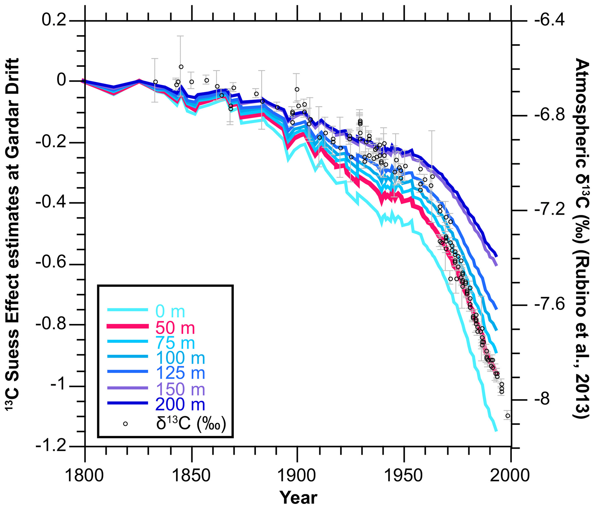
Figure 2 ¹³C Suess effect estimates at the Gardar Drift (60.5° N, 23.5° W) for the 10 different depth layers from the surface to 200 m, plotted together with the atmospheric δ¹³C record provided by Rubino et al. (2013).

2.3 SCP analysis

We followed the SCP method outlined by Rose (1994). Approximately 0.2 g of dried bulk sediment was weighed into 15 mL polypropylene tubes. One SCP reference standard (Rose, 2008) and a blank were included for quality control purposes and treated exactly the same as the samples. The SCP extraction method included nitric acid (HNO₃), hydrofluoric acid (HF), and hydrochloric acid (HCl) stages to respectively remove organic matter, silicious material, and carbonates. Following the acid digestion stages, a known fraction of the final residue was evaporated onto a cover slip and mounted on a microscope slide using Naphrax mountant. A light microscope with 400× magnification was used to identify and count the total number of SCPs on each slide. SCP identification followed the criteria described in Rose (2008) based on morphology, color, depth, and porosity. SCP concentrations are reported as the number of SCPs per gram of dry sediment (gDM⁻¹). SCP analyses were performed at the Department of Geography, University College London. The concentration of the SCP reference material was 5318 gDM⁻¹ (±1022, 90 % confidence level), close to the reported concentration of 6005 ± 70 gDM⁻¹ (Rose, 2008). No SCPs were observed in the blank.

3 The new age model approach

3.1 Planktonic foraminiferal δ¹³C vs. the oceanic ¹³C Suess effect

In the subpolar North Atlantic, G. bulloides calcifies in the upper 50 m of the water column over the late spring and summer, depending on food availability (Jonkers et al., 2013; Schiebel et al., 1997; Spero and Lea, 1996; Chapman, 2010). On the other hand, the habitat depth of N. incompta is highly variable, ranging from the surface to deeper thermocline, most likely calcifying between 50 and 125 m water depth (Chapman, 2010; Field, 2004; Pak and Kennett, 2002; Pak et al., 2004; Von Langen et al., 2005; Nyland et al., 2006; Schiebel et al., 2001). G. inflata is a deep-dwelling foraminiferal species, living at the base of the seasonal thermocline or deeper in the main thermocline if the base of the seasonal thermocline is warmer than 16 °C (Cléroux et al., 2007). In the North Atlantic, G. inflata calcifies between 200 and 400 m south of 57° N and between 100 and 200 m north of 57° N (Ganssen and Kroon, 2000).

To calculate the age estimates based on the ¹³C Suess effect, we assume a calcification depth of 50 m for G. bulloides and compare our G. bulloides δ¹³C record with the ¹³C Suess effect change at 50 m (δ¹³C_{SE_50}) at our core location. In order to avoid any uncertainties regarding planktonic foraminiferal depth habitats, we also present a stacked planktonic δ¹³C record (δ¹³C_stack – i.e., the average of G. bulloides, N. incompta, and G. inflata) and compare it with the average ¹³C Suess effect change over the top 200 m of the water column (δ¹³C_{SE_0–200}), which spans the depth habitats of all three planktonic species (i.e., G. bulloides, N. incompta, and G. inflata) used in this study (Figs. S1 and S2 in the Supplement).

3.1.1 G. bulloides δ¹³C vs. oceanic Suess effect change at 50 m (δ¹³C_{SE_50})

The G. bulloides δ¹³C record shows large natural variability over the 10–44 cm core interval, varying between ∼ 0.08 ‰ and ∼ −0.6 ‰. However, the most prominent feature occurs towards the core top. δ¹³C values reach a peak of 0.27 ‰ at 7.5 cm, then start to gradually decrease and reach 0.05 ‰ at 1 cm. This is followed by a very sharp decline of ∼ 0.8 ‰ centered at 0.5 cm. The gradual decrease observed in G. bulloides δ¹³C, with a sharper decline at the core top, indicates the presence of the ¹³C Suess effect. Compared to the ¹³C Suess effect change at 50 m, the relative change in G. bulloides δ¹³C seems to be very similar (Fig. S3 in the Supplement). Does the δ¹³C_{SE_50} curve provide a means to narrow down chronological uncertainties over the industrial period? To explore this, we objectively matched our G. bulloides δ¹³C record with the δ¹³C_{SE_50} curve to find the starting point (1800 CE) of the Suess effect curve on the G. bulloides δ¹³C record.

To objectively place the start of the δ¹³C_{SE_50} curve (1800 CE) on the G. bulloides δ¹³C record, first we computed the curvature of the δ¹³C_{SE_50} curve. We use a third-degree polynomial fit using the polyfit function in MATLAB. Secondly, we apply third-degree polynomial curve fits to the G. bulloides δ¹³C record for different core depth intervals (n=12) starting from 12 cm to cover the whole industrial period. We apply curve fits to 12–0, 11–0, 10–0, 9–0, 8.5–0, 8–0, 7.5–0, 7–0, 6.5–0 6–0, 5.5–0, and 5–0 cm intervals. When applying curve fits, we use G. bulloides δ¹³C, as well as its three-point running mean and five-point running mean, assuming the overall trends might be better represented in the smoothed data. Goodness-of-fit results for each curve fit are presented in Table S1 in the Supplement. Finally, we compared the curvature of the δ¹³C_{SE_50} curve with the various curve fits applied to G. bulloides δ¹³C records to find which curve fit is the most similar to the curvature of δ¹³C_{SE_50}. To do this, we calculate the correlation coefficients between our target curve (in this case, the curvature of δ¹³C_{SE_50}) and each of the third-degree polynomial curves using their individual polynomial coefficients (i.e., p1, p2, p3, p4; Table S1). The curvature of the G. bulloides δ¹³C record for the 7.5–0 cm interval is the most similar to the curvature of our δ¹³C_{SE_50} curve (r = 0.73), suggesting 7.5 cm could be 1800 CE. We further do the same test using the three-point and five-point running mean of the data. Although the correlation is poorer, the same result is also reached (i.e., best fit when the record starts at 7.5 cm) when three-point running mean (r = 0.46) and five-point running mean (r = 0.22) of G. bulloides δ¹³C are used. Placing the start of the oceanic Suess effect change (∼ 1800 CE) on our G. bulloides δ¹³C record is one of the main challenges of our approach as the most prominent δ¹³C decline does not happen until the most recent years or core top. This is also evident from our correlation analysis results (Table S1). For instance, a close second-best fit occurs when we place 1800 CE at 5 cm (r = 0.69) instead of 7.5 cm (r = 0.73). A comparison between the two correlation coefficients using the Fisher's z transformation suggests that the difference between the correlation coefficients is not statistically significant (z = 0.064, p = 0.949). This indicates that 5 cm could also be 1800 CE.

3.1.2 δ¹³C_stack vs. the 0–200 m average oceanic Suess effect change (δ¹³C_{SE_0–200})

N. incompta and G. inflata δ¹³C also followed a very similar trend as the G. bulloides δ¹³C record – with the most prominent decline towards the core top, indicating the presence of the ¹³C Suess effect. To cross-check our approach described in Sect. 3.1.1 and to avoid any uncertainties that may be caused due to habitat depth variability, we use the stacked planktonic δ¹³C of G. bulloides, N. incompta, and G. inflata (δ¹³C_stack). Considering the habitat depth range of all three planktonic species, we then compare the δ¹³C_stack with the 0–200 m average of the ¹³C Suess effect (δ¹³C_{SE_0–200}) (Figs. S1 and S2). Similarly, to place the start of the δ¹³C_{SE_0–200} curve (1800 CE) on our δ¹³C_stack record, first we find the curvature of the δ¹³C_{SE_0–200} curve. We use a third-degree polynomial fit using the polyfit function in MATLAB. Secondly, we apply third-degree polynomial curve fits to the δ¹³C_stack record for the same core depth intervals as in Sect. 3.1.2. Finally, we compare the curvature of the Δ¹³C_{SE_0–200} curve with the various curve fits applied to our δ¹³C_stack record and find which curve fit is the most similar to the curvature of Δ¹³C_{SE_0–200}. To do this, we again calculate the correlation coefficients between our target curve (in this case, the curvature of δ¹³C_{SE_0–200}) and each of the third-degree polynomial curves using their individual polynomial coefficients (i.e., p1, p2, p3, p4; Table S1). In this case, we get similar results for intervals 5–0, 5.5–0, and 7.5–0 cm (r = −0.60). Although the negative correlation coefficients indicate that the similarity approach used here may not capture the complexity of comparing third-degree polynomials, it gives us a rough estimate of which curve is most similar to our target curve (i.e., Δ¹³C_{SE_0–200}) and overall agrees with our initial finding based on G. bulloides that 7.5 or 5 cm may in fact be 1800 CE.

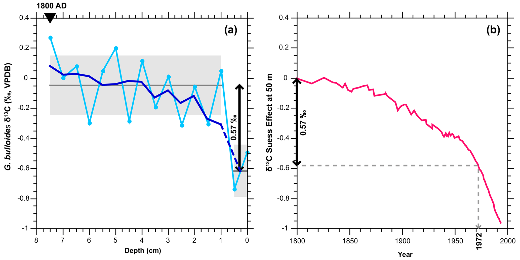
Figure 3 Overview of core-top age calculation. (a) G. bulloides δ¹³C record (blue, with five-point mean; bold line) vs. depth (cm). The five-point mean is extended into the core top by taking the mean of samples at 0 and 0.5 cm, shown as dashed bold lines to highlight the large abrupt δ¹³C decrease at the core top. The dark gray line and gray shading respectively mark the mean and standard deviation of the 1–7.5 cm and 0 and 0.5 cm intervals. (b) δ¹³C_{SE_50} curve (pink). The arrow and dashed lines mark when a 0.57 ‰ magnitude decline occurs in the record.

3.2 Core-top age

In paleoceanographic studies it is common to use the year a sediment core was retrieved as the core-top age. However, this is highly dependent on the sedimentation rates of the region and may not always be the case. The core-top (0 cm) ¹⁴C AMS date for GS06-144-09 MC-D indicated the presence of bomb carbon, confirming that the top should be younger than ∼ 1957 CE (Mjell et al., 2016). Therefore, based on high sedimentation rates at the site, Mjell et al. (2016) assumed 2006 CE to be the core-top age, i.e., the year core GS06-144-09 MC was retrieved. Here we explore this further considering the new information provided by the relative change in our oceanic ¹³C Suess effect curve. For this, we use the G. bulloides δ¹³C record and the δ¹³C_{SE_50} curve.

Based on our previous curve fits, we place 1800 CE at 7.5 cm. The most prominent change in the G. bulloides δ¹³C record occurs at 0.5 cm. Hence, first we find the mean and standard deviation of the 1–7.5 cm interval (−0.05 ± 0.2; n=14), i.e., the mean δ¹³C over the industrial period and secondly the core top (two data points at 0 and 0.5 cm; −0.62 ± 0.17; n=2), of the G. bulloides δ¹³C record, i.e., where the sharpest decline due to the Suess effect occurs. We then calculated the difference in means using a t test (0.57 ‰) and found the magnitude of the sharpest decline in G. bulloides δ¹³C due to the Suess effect. Finally, we used the δ¹³C_{SE_50} curve to find when a 0.57 ‰ magnitude decline relative to the preindustrial value occurred. Based on our δ¹³C_{SE_50} curve, a decline of 0.57 ‰ occurs in ∼ 1972. This would then place 1972 CE at 0.25 cm (i.e., the mid-point of our two samples at 0 and 0.5 cm), suggesting a much older core-top age than previously assumed for GS06-144-09 MC (Mjell et al., 2016).

We repeated the same approach and evaluated how the core-top age would change if we placed 1800 CE at 5 cm (i.e., our second-best fit). We computed the mean and standard deviation of the 1–5 cm interval (−0.09 ± 0.2; n=9) and calculated the difference in means (0.53 ‰) between the 1–5 cm interval and the core top (0–0.5 cm). Finally, we determined when a magnitude of 0.53 ‰ decline occurred in the δ¹³C_{SE_50} curve. Based on our δ¹³C_{SE_50} curve, a decline of 0.53 ‰ occurred in ∼ 1969, placing 1969 CE at 0.25 cm. This suggests that placing 1800 CE at 7.5 cm vs. 5 cm changes our core-top age (or our tie point at 0.25 cm) by 3 years. When building our age model, here we choose 7.5 cm as 1800 CE (i.e., based on the best curve fit) and 0.25 cm as 1972 CE, and we introduce 3-year uncertainty to the selection of these tie points.

3.3 Revising regional reservoir corrections (ΔR) at Gardar Drift

To build an age model for the marine sediment cores based on radiocarbon dating it is necessary to convert ¹⁴C dates into calendar years. Surface ocean ¹⁴C is depleted relative to the atmosphere, which is known as the marine reservoir effect. Global marine radiocarbon calibration curves, e.g., the latest Marine20 curve (Heaton et al., 2020), account for the global average offset between the marine and atmospheric reservoirs; however, there are temporal and spatial deviations from this offset. Marine reservoir ages range from 400 years in the subtropics to more than 1000 years in polar oceans (Key et al., 2004). Therefore, the accurate calibration of ¹⁴C ages depends on knowledge of the local radiocarbon reservoir age of the surface ocean, i.e., the regional difference (ΔR) from the global marine radiocarbon calibration curve. The marine reservoir database within CALIB (http://calib.org/marine/, last access: 1 November 2023) is the most extensive and valuable source for ΔR values for the modern ocean (Reimer and Reimer, 2001; Stuiver and Reimer, 1986). This online platform provides the user with an average ΔR value for their core location based on the information provided on coordinates and number of nearest points. The ΔR values within the marine reservoir database are determined based on the known-age approach, i.e., when the death date (in calendar ages) of a pre-bomb marine sample (e.g., a mollusk shell) is known. However, as a consequence of nuclear tests in the 1950s and early 1960s the ΔR calculation with the known-age approach can only be applied to samples collected before 1950 CE; hence, the majority of the samples within the marine reservoir database are not homogenously distributed – making them temporally and spatially limited (Alves et al., 2018). Therefore, deriving a ΔR using the nearest points to a core location is problematic for many regions, where the closest ΔR is either not available or located in a different oceanographic setting (e.g., Hinojosa et al., 2015). When selecting samples for ΔR calculation, it is also important to review the ecological information on the taxa from which the ΔR value is derived, as some studies find species-specific values due to habitat, feeding mechanisms, and food sources. For instance, suspension feeders are thought to be the most suitable for dating, whereas deposit feeders, omnivore species, or carnivorous species are generally excluded due to their greater uncertainty in ¹⁴C ages as they incorporate old carbon (Pieńkowski et al., 2021; England et al., 2013; Forman and Polyak, 1997). However, some studies find no difference in ¹⁴C ages due to feeding mechanisms when the mollusks are derived from areas with no carboniferous rocks or local freshwater inputs to the surface ocean (Ascough et al., 2005).

Table S2 in the Supplement shows the ΔR values for our core site (GS06-144-09 MC; 60°19^′ N, 23°58^′ W), located south of Iceland, derived from the nearest points available in the marine reservoir database (Reimer and Reimer, 2001). When the 10 nearest points are used (i.e., based on the distance (km) from core location), the ΔR for our core site is −72 ± 64 ¹⁴C yr. However, when we exclude carnivore and deposit feeding species, the ΔR value becomes −80 ± 54 ¹⁴C yr. It is also important to note that even the individual samples have a large range of ΔR values, varying between −23 ± 45 and −220 ± 85 ¹⁴C yr, suggesting there might be other factors influencing the ΔR. For instance, considering the oceanographic setting, another approach could be to only select samples located around southern Iceland – i.e., those potentially under the influence of the Irminger Current, where our core site lies. Then, the ΔR value would be −92 ± 93 ¹⁴C yr (or −126 ± 66 ¹⁴C yr when carnivore and deposit feeding species are excluded). This suggests that the available ΔR values within the CALIB marine reservoir database (Reimer and Reimer, 2001) for the region are highly variable and highly dependent on the selection criteria used by the investigator.

Global Ocean Data Analysis Project (GLODAP) radiocarbon observations (Key et al., 2004) provide an alternative approach to estimate the spatial variations in the reservoir ages (Gebbie and Huybers, 2012; Waelbroeck et al., 2019). For instance, Waelbroeck et al. (2019) extracted the pre-bomb surface mean (upper 250 m) reservoir ages from re-gridded (4° × 4°) GLODAP data. Following the Waelbroeck et al. (2019) approach, we extract the reservoir ages (443 ± 75.8 ¹⁴C yr) at our core site (60° N, 24° W) from GLODAP data. Waelbroeck et al. (2019) note, however, that the error for their reservoir ages should be at least 100 ¹⁴C yr if the computed GLODAP standard deviation is less than this value (i.e., in our case 443 ± 100 ¹⁴C yr). Considering the global average marine reservoir age of ∼ 600 years based on Marine20 (Heaton et al., 2020), this would suggest a ΔR of −157 ± 100 ¹⁴C yr for our region. The large difference (and/or uncertainties) in regional reservoir corrections extracted using two independent methods (e.g., CALIB vs. GLODAP-based) highlights the need for additional approaches to further constrain regional reservoir ages.

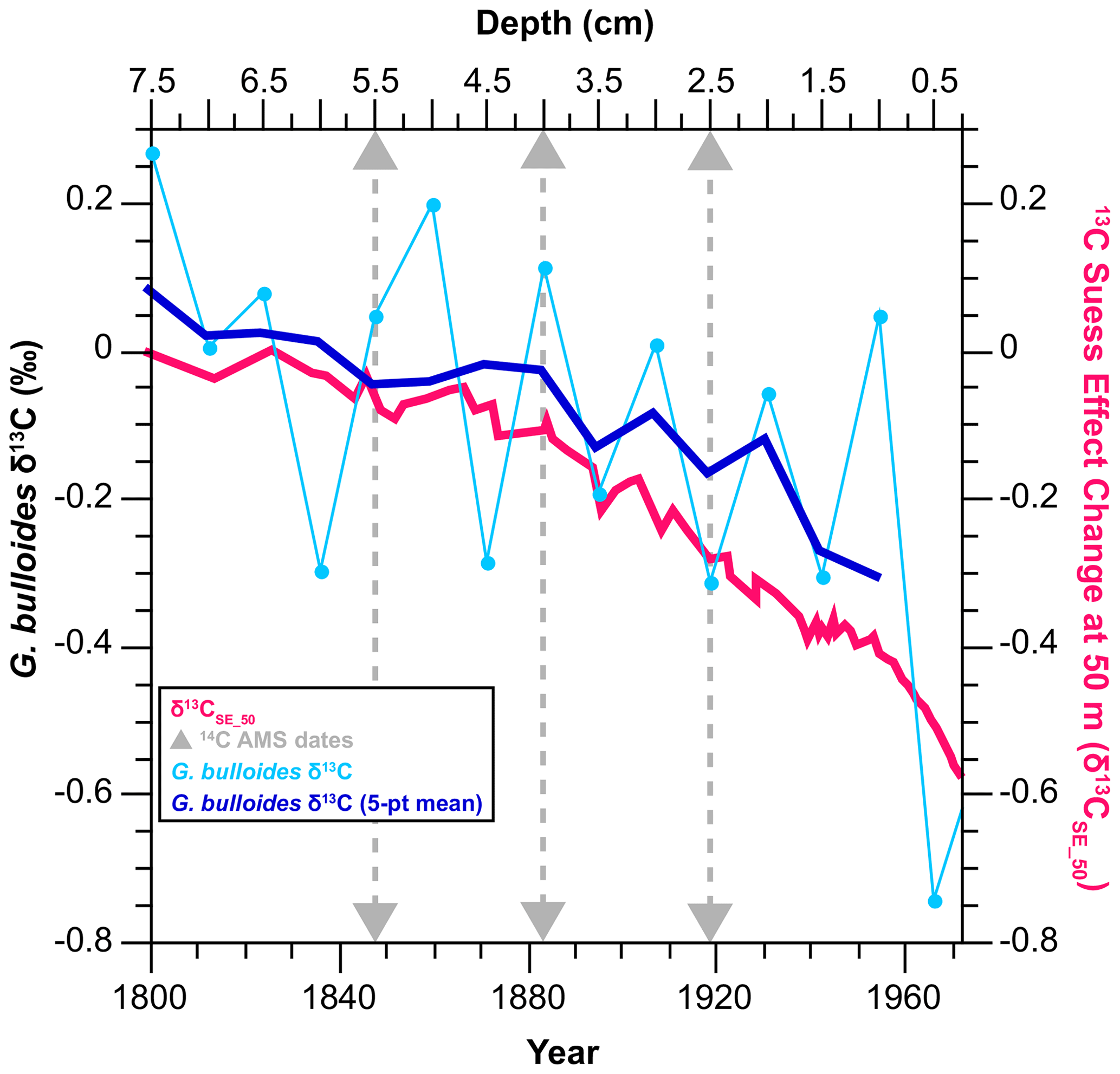
Figure 4 G. bulloides δ¹³C (7.5–0.25 cm, light blue line plotted with the five-point mean; bold dark blue line) vs. the δ¹³C_{SE_50} curve spanning the 1800–1972 CE interval (bold pink line). Gray triangles on the depth axis mark the three ¹⁴C AMS samples at 2.5, 4, and 5 cm depth intervals, while the dashed gray lines and triangles on the age axis mark their corresponding “known ages” based on the Δ¹³C_{SE_50} comparison.

Here we suggest an alternative approach for calculating the ΔR for marine sediment cores that is independent of uncertainties such as the distance between core sites and sample locations, different oceanographic settings (e.g., coastal and fjord regions vs. open ocean), or the feeding ecology of the species used for dating. Based on our comparison of the G. bulloides δ¹³C record and the δ¹³C_{SE_50} curve we obtain two tie points, placing 1972 CE at 0.25 cm and 1800 CE at 7.5 cm. Figure 4 shows the G. bulloides δ¹³C record on a depth scale spanning the 7.5–0.25 cm core interval, plotted together with the δ¹³C_{SE_50} curve spanning the 1800–1972 CE interval. First, we estimate the “known ages” for depths 2.5, 4, and 5.5 cm (i.e., where we have ¹⁴C dates) by reading the corresponding ages from the δ¹³C_{SE_50} curve. Next, we calculate the ΔR value for each sample using the known-age approach in the online application deltar (Reimer and Reimer, 2017) based on the most recent Marine20 curve (Heaton et al., 2020). Finally, we calculate the weighted mean (Eq. 2) and standard deviation of ΔR following Reimer and Reimer (2001) and provide a revised ΔR estimate for the Gardar Drift. The uncertainty of ΔR is determined as the maximum value of either the weighted uncertainty in the mean of ΔR or the standard deviation of ΔR, as in Eqs. (3) and (5). Our refined ΔR estimate (−69 ± 38 ¹⁴C yr) is similar to the value obtained from the marine reservoir database when the 10 nearest points are used (−72 ± 64 ¹⁴C yr) – although with better uncertainty estimates.

$$\begin{array}{}\text{(2)}& {\displaystyle }\begin{array}{rl}\text{Weighted\hspace{0.17em}\hspace{0.17em}mean\hspace{0.17em}\hspace{0.17em}of }& \mathrm{\Delta }R=\mathit{\mu }={\displaystyle \frac{{\sum }_i\frac{\mathrm{\Delta }{R}_i}{{\mathit{\sigma }}_i^{\mathrm{2}}}}{{\sum }_i\frac{\mathrm{1}}{{\mathit{\sigma }}_i^{\mathrm{2}}}}};\\ & \text{ where }{\mathit{\sigma }}_i\text{ is\hspace{0.17em}\hspace{0.17em}the\hspace{0.17em}\hspace{0.17em}uncertainty\hspace{0.17em}\hspace{0.17em}in }\mathrm{\Delta }{R}_i\end{array}\text{(3)}& {\displaystyle }\text{Weighted\hspace{0.17em}\hspace{0.17em}uncertainty\hspace{0.17em}\hspace{0.17em}in\hspace{0.17em}\hspace{0.17em}mean\hspace{0.17em}\hspace{0.17em}of }\mathrm{\Delta }R={\displaystyle \frac{\mathrm{1}}{{\sum }_i\frac{\mathrm{1}}{{\mathit{\sigma }}_i^{\mathrm{2}}}}}\text{(4)}& {\displaystyle }\text{Variance\hspace{0.17em}\hspace{0.17em}of }\mathrm{\Delta }R={\displaystyle \frac{\frac{\mathrm{1}}{n-\mathrm{1}}\cdot {\sum }_i{\left(\frac{\mathrm{\Delta }{R}_i-\mathit{\mu }}{{\mathit{\sigma }}_i}\right)}^{\mathrm{2}}}{\frac{\mathrm{1}}{n}\cdot {\sum }_i\frac{\mathrm{1}}{{\mathit{\sigma }}_i^{\mathrm{2}}}}}\text{(5)}& {\displaystyle }\text{Standard\hspace{0.17em}\hspace{0.17em}deviation\hspace{0.17em}\hspace{0.17em}of }\mathrm{\Delta }R=\sqrt{\text{variance}}\end{array}$$

Table 2 Revised ΔR estimate for Gardar Drift. “Known ages” are derived from the ¹³C Suess effect comparison, as shown in Fig. 4. The weighted mean and standard deviation of ΔR are calculated following the method outlined in CALIB using Eqs. (2)–(5) (Reimer and Reimer, 2017, 2001).

3.4 Revised age model for GS06-144-09 MC

We use Bacon (version 2.5.0), the age–depth modeling approach that uses Bayesian statistics (Blaauw and Christen, 2011), operated through R (version 4.0.3) – free software for statistical computing and graphics. A total of 10 ¹⁴C AMS dates (Table 1) are calibrated through Bacon using the most recent Marine20 curve (Heaton et al., 2020) and a ΔR value of −69 ± 38 (this study) – assuming a constant ΔR value throughout the core. Since our ΔR estimate is based on the comparison with the ¹³C Suess effect curve, we can only calculate a ΔR value for the last ∼ 200 years with this approach. Although we assume relatively stable conditions over the last millennium (e.g., compared to glacial–interglacial changes), changes in ocean circulation and ventilation before this period will also effect the ΔR in the region (e.g., during the Little Ice Age; Spooner et al., 2020).

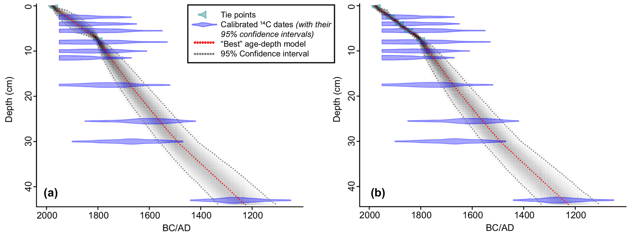
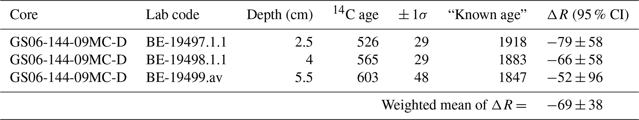
Figure 5 Age–depth plots of GS06-144-09 MC (a) when additional tie points for 0.25 cm (1972 CE) and 7.5 cm (1800 CE) are used and (b) when “known” calendar ages for samples at 2.5, 4, and 5.5 cm that were derived from the δ¹³C_{SE_50} comparison are used as additional tie points.

Additional tie points for 0.25 cm (1972 CE) and 7.5 cm (1800 CE) are used based on the information obtained from the Suess effect curve. Based on the core-top (0 cm) ¹⁴C AMS date (> 1950 CE) and the year the core was retrieved (2006 CE) the core-top age should be between ∼ 1950 and 2006 CE. As the core-top age cannot be younger than 2006 CE, we use this information as a prior in Bacon to set a minimum age limit for the core top. According to the revised age model, the date for the core top (0–0.5 cm) is 1977 CE. The average uncertainty for the last ∼ 200 years (i.e., the 0–7.5 cm interval) is ∼ ± 42 years and for the whole core (i.e., the 0–44 cm interval) is ± 90 years. The resulting age–depth plot is provided in Fig. 5a. Although Bacon selects the best age–depth model (i.e., dotted red lines in Fig. 5), considering the sedimentation rate profile based on the prior information, the tie points at the core top and 1800 CE play a crucial role, providing a basis for sedimentation rates. This is also seen from Fig. 5a, illustrated by the large range of ¹⁴C AMS dates that exceeds the calibration range of Marine20 due to bomb carbon. This further underscores the need for independent chronological approaches, particularly for the last century.

As a comparison, we also include the “known” calendar ages for samples at 2.5, 4, and 5.5 cm that were derived from the δ¹³C_{SE_50} comparison, together with their uncalibrated ¹⁴C dates, in the Bacon input file. For all the tie points derived from the δ¹³C_{SE_50} comparisons we add a ± 3-year uncertainty. Including the known calendar ages does not change the overall age model, but as expected, it highly decreases the age model uncertainties for the last ∼ 200 years (Fig. 5b). Based on this, the core-top age (0–0.5 cm) is again 1977 CE. The average age model uncertainty for the last ∼ 200 years (i.e., the 0–7.5 cm interval) is ± 17.5 years. Below this point, the uncertainty increases (average of ± 84 years for the 0–44 cm interval) and is highly dependent on the uncertainty of the ¹⁴C AMS dates. The average sedimentation rates for the top 0–7.5 cm interval are 43 and 63 cm kyr⁻¹ for the 7.5–44 cm interval. The average sedimentation rate of the core (0–44 cm) is 59 cm kyr⁻¹, giving a sample spacing of ∼ 8.5 years per 0.5 cm sample.

3.5 SCP analysis

To cross-check the validity of our Suess-effect-derived age model, here we use another independent approach: spheroidal carbonaceous fly-ash particles (SCPs).

SCP concentrations at GS06-144-09 MC are generally very low, varying between 152 and 616 gDM⁻¹. Based on our revised age model, SCP concentrations start to gradually increase during the 1930s. A more marked increase in SCP concentrations occurs after 1954 and reaches peak values in 1966, followed by a decline towards the core top. Figure S4 in the Supplement shows a comparison of the GS06-144-09 MC SCP concentrations with previously published SCP profiles from Apavatn Lake, Iceland (Rose, 2015), and Nunatak Lake, Greenland (Bindler et al., 2001; Rose, 2015). Despite similarly low concentrations, both lake records show the same increase after ca. 1950 as the Gardar Drift marine sediment core. This suggests that the SCP concentrations at Gardar Drift follow a similar temporal pattern to the lake sediments in the region. Although the low SCP concentrations at GS06-144-09 MC result in considerable uncertainty for the SCP profile, the rapid increase after the 1950s at GS06-144-09 MC is consistent with the SCP trend in the region and is consistent with our Suess-effect-based revised age model.

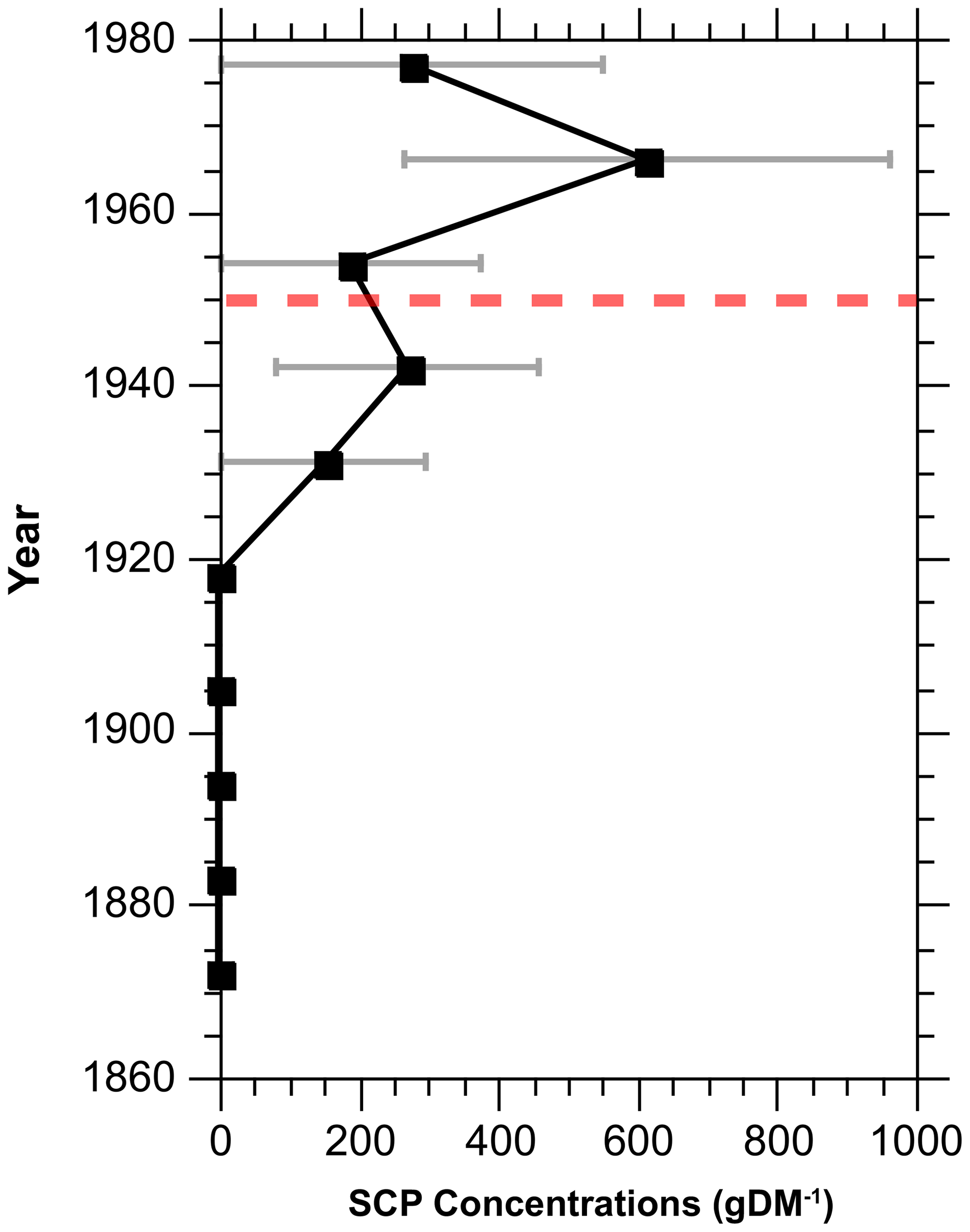
Figure 6 SCP concentration profile of GS06-144-09 MC plotted vs. the revised age model (as shown in Fig. 5b). The dashed red line marks 1950.

Figure 7 Age–depth plot for the top 10 cm of GS06-144-09 MC to highlight the differences (e.g., in sedimentation rate) between the original ²¹⁰Pb-based chronology (Mjell et al., 2016) and the tie points derived based on anthropogenic signals (this study). ¹⁴C dates are calibrated with CALIB (version 8.2) (Stuiver and Reimer, 1993) using Marine20 and ΔR = −69 ± 38 ¹⁴C yr.

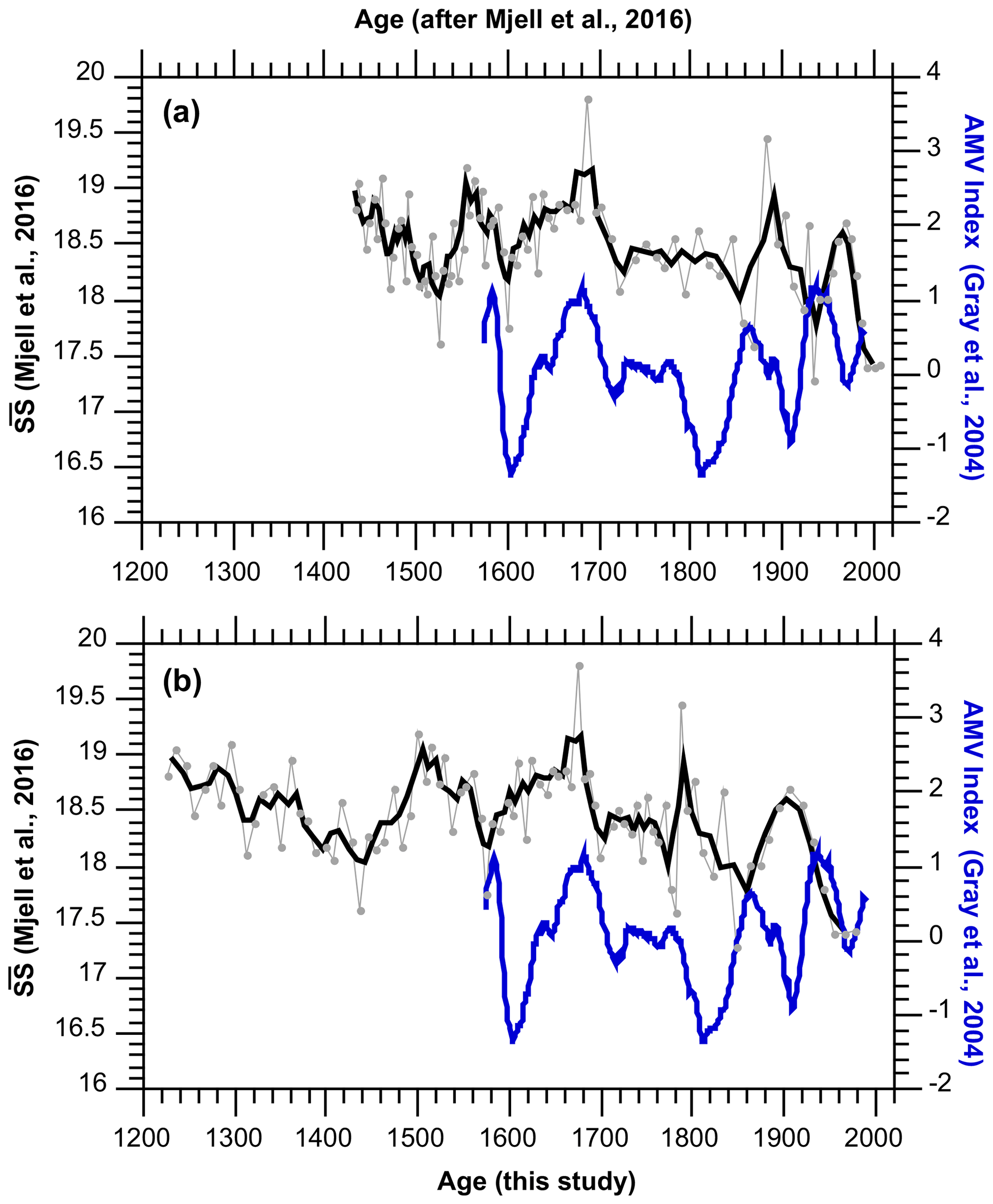
Figure 8 Sortable silt mean grain size ($\stackrel{\mathrm{‾}}{\mathrm{SS}}$) as a proxy for Iceland–Scotland Overflow Water vigor (Mjell et al., 2016) vs. the AMV index (Gray et al., 2004), plotted on the (a) original age model (after Mjell et al., 2016) and (b) revised age model using anthropogenic signals (this study).

4 Discussion

Our case study off Gardar Drift demonstrates the utility of two novel chronostratigraphic approaches that use anthropogenic signals (i.e., the oceanic ¹³C Suess effect change and SCP concentrations) in reducing age model uncertainties of recent high-resolution marine archives. In addition, using a combination of ¹⁴C AMS dates and oceanic ¹³C Suess effect estimates, we further provide refined regional ¹⁴C reservoir corrections and uncertainties for Gardar Drift. Despite the similarity of our refined ΔR estimate to those available in the marine reservoir database (Reimer and Reimer, 2001), it is also important to note the shortcomings of our approach. For instance, by reading the corresponding known ages from the ¹³C Suess effect curve to calculate ΔR, our approach assumes constant sedimentation rates and no bioturbation or reworking at the core top. Although we do not see any visible traces of bioturbation in our core, we acknowledge that this is often not the case, and we rarely have sites with true known ages. One exception to this, with potential to overcome this limitation, would be to use absolute age markers derived by identifying tephra layers and fingerprinting these to known volcanic eruptions. Yet this method is also only applicable in specific geologic settings and can also be affected by bioturbation – a limitation shared by all dating methods.

Bioturbation is one of the main sources of uncertainties of our approach as it will typically influence the age distributions and smooth the record. Generally, the smoothing, or attenuation, is greater when the sedimentation rates are low (∼ 10 cm kyr⁻¹) (Anderson, 2001). For instance, according to Anderson (2001) minimum attenuation (i.e., < 5 %) is observed only when sedimentation rates exceed 50–70 cm kyr⁻¹ – a range often observed at sedimentary drift sites, such as the Gardar Drift. Given the average sedimentation rate of ∼ 43 cm kyr⁻¹ for the top 0–7.5 cm interval of our core (i.e., spanning an interval from ca. 1977 to 1800 CE) and sampling resolution of 0.5 cm, our ultimate chronological precision potentially achievable using these methods would be ∼ 12 years.

We further compare our revised age model based on anthropogenic signals with the previously published age model for Site GS06-144-09 MC-D. Figure 7 shows the ²¹⁰Pb dates (Mjell et al., 2016), ¹⁴C dates, and information provided by the anthropogenic signals (i.e., ¹³C Suess-effect-derived tie points and the interval where the SCPs are present). The significant mismatch between the ²¹⁰Pb and ¹⁴C dates once again highlights the need for independent approaches, as well as the potential of using anthropogenic signals to improve age model constraints over the last 2 centuries.

One of the main differences between our revised age model and that of Mjell et al. (2016) is the core-top age (1977 vs. 2006, respectively). This once more emphasizes the need to validate ²¹⁰Pb-based chronologies as well as the common assumption of the year a sediment core was retrieved as the core-top age. Here we suggest and assume that the significant decline in our foraminiferal δ¹³C records over the last century is mainly caused by the oceanic ¹³C Suess effect. This is particularly the case for our G. bulloides δ¹³C, where the actual decline in foraminiferal δ¹³C is the same as the ¹³C Suess effect decline at 50 m depth. However, this may also be registered differently in other species. It is important to note that, although difficult to distinguish, our foraminiferal δ¹³C signals are also subject to natural climate variability. For instance, there are significant changes in the subpolar gyre circulation over the 20th century; more specifically, the observed productivity decline in the region (Spooner et al., 2020) will also be registered by our foraminiferal δ¹³C. Here, we have focused on the relative difference between average G. bulloides δ¹³C values over the industrial period vs. the core top (i.e., sharpest ¹³C decline due to the Suess effect) and demonstrated the potential utility of the ¹³C Suess effect approach in recent marine sediment chronologies. However, further sensitivity studies are needed to distinguish the effects of natural vs. anthropogenic climate variability in foraminiferal δ¹³C records.

The scale of the, ongoing, Suess effect is now starting to exceed the entire range of δ¹³C exhibited through most open-ocean environments (Eide et al., 2017), and, as such, it should be a dominant feature in records able to resolve short timescales. Indeed, the lack of this signal in a core-top record suggests that modern sediments were not recovered and/or that sedimentation rates and bioturbation may confound sub-centennial-scale interpretation of foraminiferal isotope records at a given core site.

Finally, Fig. 8 shows the sortable silt record of Mjell et al. (2016) on its original age model that is based on ²¹⁰Pb and two ¹⁴C dates vs. the revised age model (as shown in Fig. 5b) for GS06-144-09 MC-D, plotted together with the AMV index (Gray et al., 2004), to illustrate how our proxy-based interpretations for the 20th century might change with revised marine sediment chronologies.

Although marine based uncertainties over the last 2 centuries might still be too high (∼ ± 18 years in average) for a significant lead–lag comparison with observational records, our new approach based on anthropogenic signals provides an independent and valuable first step in refining age models and for validation of existing age model approaches and their assumptions.

5 Summary and conclusions

High-resolution (i.e., decadal to multi-decadal) marine sediment records from North Atlantic sedimentary drift sites are now emerging, with the potential to extend instrumental records further back in time, distinguish natural climate variability from anthropogenic variability, and contextualize current changes. However, age model uncertainties, particularly over the 20th century, pose major challenges, especially for integrating shorter instrumental records with those from extended marine archives. Recent sediments are dated using an array of methodologies, yet all have their own limitations (e.g., bomb carbon, local reservoir corrections for radiocarbon); they are either not applicable to all locations (e.g., tephrochronology) or can be below the detection limits and require another independent approach to confirm (e.g., ²¹⁰Pb, ³⁷Cs). Here we propose a new chronostratigraphic approach that uses anthropogenic signals to reduce age model uncertainties over the last 2 centuries. As a test application, we use the Gardar Drift sediment core GS06-144-09 MC and revise the age model at this site. Comparing planktonic δ¹³C records of GS06-144-09 MC with oceanic ¹³C Suess effect changes above the core location, we assign the beginning of the industrial period (i.e., 1800 CE) in our core and similarly derive the core-top age. We further use a combination of ¹⁴C AMS dates and the ¹³C Suess effect change estimates at our core location to calculate regional reservoir corrections at Gardar Drift. Our refined ΔR estimate for Gardar Drift (−69 ± 38 ¹⁴C yr) is similar to the value obtained from the marine reservoir database when the 10 nearest points are used (−72 ± 64 ¹⁴C yr) but with better uncertainty estimates. Furthermore, to validate our ¹³C Suess-effect-based age model we use another independent approach: spheroidal carbonaceous fly-ash particles (SCPs). The rapid increase in SCP concentrations after the 1950s at GS06-144-09 MC is consistent with the SCP trend in the region and our ¹³C Suess-effect-based age model. Our new approach, based on anthropogenic signals, provides an independent and valuable first step in refining age models and for validation of existing age model approaches and their assumptions.