Measuring varve thickness using micro-computed tomography (µCT): a comparison with thin section

X-ray micro-computed tomography (µCT) scans were performed on four varved sediment cores collected in Grand Lake (Labrador) and previously studied with thin sections. These scans allowed us to investigate the possibility of using µCT as a substitute for thin sections to carry out counts and thickness measurements of varved sediments. Comparing varve counts of these two methods, µCT counts are slightly higher than the ones made with thin sections. The difference in counts suggests that the petrographic study and a scanning electron microscope (SEM) analysis of a thin section remain necessary for determining the varve character of the laminae. Yet, µCT allows measurements in multiple directions, improving the robustness of the counts and avoiding the manufacturing of continuous thin sections along a sediment sequence. As for the thickness measurement, the µCT analyses were made in two perpendicular directions. Not surprisingly, measurements made on the same cutting plane as the thin section are quite similar to the ones made on the latter. However, there are significant differences with measurements made on the perpendicular plane. This highlights the need to perform varve thickness measurements in at least two perpendicular directions for better estimates of varved sediment thicknesses. In addition, the study illustrates that µCT is an effective way to select the least deformed zones with parallel varves to carry out the best possible thickness measurements.

1 Introduction

Examinations of sediment cores from lakes and oceans have provided insight into climate change and natural climate variation in different parts of the world through reliable paleoclimate reconstructions. These reconstructions required thorough examinations of sedimentary facies' structure and texture. Varves are among the most influential sedimentary facies for paleoclimatic reconstructions. The term varve refers to a set of layers formed annually (Kemp, 1996; Hughen, 2013; De Geer, 1912). These annual sedimentation facies form cyclically in marine or lacustrine environments, with origins ranging from detrital, endogenous, or biogenic to a combination of these processes (Zolitschka et al., 2015; Schimmelmann et al., 2016). Detrital varves are the object of study in this project. They often show a regular alternation of light and dark beds of different grain sizes, with millimetric thicknesses (Ojala et al., 2012; Zolitschka et al., 2015). The advantage of studying varves is that they are high-resolution sedimentary sequences providing information on past abrupt environmental changes through variations in the structure, composition, and thickness of their distinct seasonal laminae (Ojala et al., 2012). The variations in structures and the thickness of their seasonal laminae can be the result of several independent factors, such as melting of snow or landslides. Yet, with a good understanding of the sedimentary components of varves and the mechanisms controlling their formation, they can be good paleoclimate indicators (Gagnon-Poiré et al., 2021; Amann et al., 2017; Palmer et al., 2019; Hardy et al., 1996).

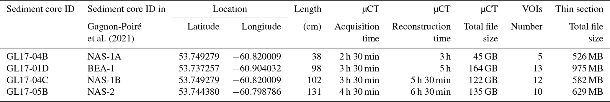
Table 1 Summary of the four sediment cores with the µCT acquisition and reconstruction time.

In addition, varved sediments contain their own chronology, which can be converted into calendar years with exceptionally high temporal resolution. Ultimately, they offer the possibility of calculating sediment flux rates (Ojala et al., 2012; Zolitschka et al., 2015; Emmanouilidis et al., 2020).

To analyse these varved sediments, the thin-section method is the most commonly used. To do this, the sediment core is continuously sampled by subsampling overlapping sediment blocks. These subsamples are then freeze-dried, impregnated with epoxy resin, and cut into blocks to make thin sections (Normandeau et al., 2019; Francus and Asikainen, 2001). The process of counting and measuring varves is then done by image analysis of thin sections at the petrographic microscope and/or using scanning electron microscope (SEM) images in backscattered mode to improve the ability to define varve boundaries (Francus et al., 2008; Lapointe et al., 2019; Gagnon-Poiré et al., 2021; Soreghan and Francus, 2004). However, the sampling method, as well as the multiple steps needed for the preparation of thin sections, can induce sediment perturbations. This is because, for fine sediments, extracting the subsample can be difficult due to their stickiness. It therefore requires a great deal of meticulousness to separate them from the underlying sediment core without tampering with them and to avoid any disturbances during the various stages of manufacturing the thin section (Normandeau et al., 2019).

Finally, there is the question of the representativeness of the sample analysed: it has limitations associated with its 2D view (Bendle et al., 2015), which make it difficult to estimate the true thickness of the varves. However, X-ray micro-computed tomography (µCT) allows the observation of objects with a resolution of a few micrometres and has the advantage of being a non-destructive technique. It allows viewing a volume instead of a plane, facilitating the study of the internal structures and orientation of a wide variety of geological objects (Cnudde and Boone, 2013; Voltolini et al., 2011; Bendle et al., 2015; Lisson et al., 2023; Cornard et al., 2023; Fabbri et al., 2024). This article aims to investigate the possibility of using (µCT) as an analytical tool to measure varves in the framework of paleoclimatic studies. To do this, we tested the µCT method on a sequence whose varves are easy to recognize, thick, and not very disturbed and which have already been studied using the thin-section method. The objectives of this paper are to (1) test if varve counts can be performed using µCT, (2) test if varve thickness can be retrieved from µCT images, (3) compare the thickness measurements obtained with those retrieved using the thin-section method, and (4) evaluate the added value of µCT as an analysis tool for varved sediments.

2 Methods

2.1 Sample selection

The study area is part of the Grenville Structural Province and is dominated by Precambrian granite, gneiss, and acidic intrusive rocks (Gagnon-Poiré et al., 2021; Trottier et al., 2020).

The analysed sediments come from Grand Lake, a 60 km long elongated lake, with a depth reaching 245 m (Trottier et al., 2020; Gagnon-Poiré et al., 2021). This fjord lake is located in a valley connected to the Lake Melville graben in the central Labrador region of Canada at 53°41^′25.38^′′ N, 60°32^′6.53^′′ W, approximately 15 m above sea level (Fig. 1) (Trottier et al., 2020; Gagnon-Poiré et al., 2021).

Grand Lake has two principal tributaries, the Naskaupi and Beaver rivers, that remobilize ancient deltaic systems and terraces composed of fluviomarine, marine, fluvioglacial, lacustrine, and modern deposits. The availability of sediments along its tributaries, combined with its great depth and high seasonal flow, has favoured the formation and preservation of fluvial clastic laminated sediments (Gagnon-Poiré et al., 2021). Thereby, it is an excellent lake for the preservation of recent records of stratified fluvial clastic sediments (Gagnon-Poiré et al., 2021; Zolitschka et al., 2015). Four undisturbed sediment sequences (Fig. A1) were extracted in front of the deltas using a Uwitec gravity corer and are listed in Table 1. After recovery, these cores were cut into two halves. The first one was used for making thin sections, and their subsequent analysis with a scanning electron microscope is reported in Gagnon-Poiré et al. (2021). The second halves are analysed in this paper using a µCT scanner.

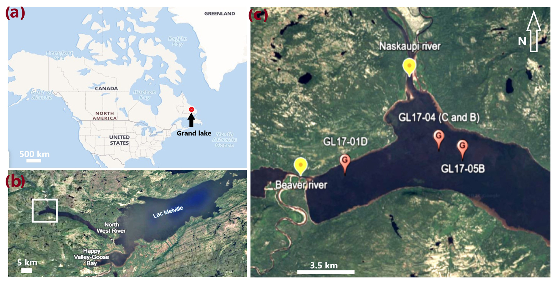
Figure 1 Study area. (a) Location of Grand Lake encircled in red on a map of Canada. (b) Location of the study area. (c) Study area with the location of the principal tributaries of Grand Lake (yellow pins) and sediment cores GL17-01D, GL17-04B, GL17-04C, and GL17-05B (© Google Earth 2023).

2.2 Measurement of varve thickness on thin sections

The making of thin sections was done in several steps (Fig. 2). First, the half sediment cores were subsampled using aluminium boxes, positioned with an overlap of approximately 1 cm to retrieve a continuous sequence along the sediment core (Francus and Asikainen, 2001).

The sediment was then frozen with liquid nitrogen to avoid the formation of large hexagonal ice crystals, which would deform the sediment. However, this step can cause cracks in the sediment block because freezing occurs too quickly (Normandeau et al., 2019). Next, the sediment was freeze-dried for 48 h to sublimate the ice without modifying the sediment structure (Normandeau et al., 2019).

The sediment was subsequently impregnated using a low-viscosity Spurr epoxy resin and hardened by thermal curing for 48 h. The final step consisted of cutting the impregnated block of sediments to manufacture thin sections (Lapointe et al., 2019). These thin sections were first digitized and analysed under a petrographic microscope. Next, images in backscattered mode were acquired using the SEM (Zeiss Evo 50) at a voltage of 20 kV (Francus et al., 2008; Gagnon-Poiré et al., 2021; Lapointe et al., 2019) with a resolution of 1 µm per pixel (Francus et al., 2002; Gagnon-Poiré et al., 2021). These 8-bit high-resolution images made it possible to count varves, providing good contrast for features which frequently measure less than 0.5 mm and are difficult to measure otherwise (Francus, 1998; Lapointe et al., 2019). Varve thicknesses are manually acquired with custom-made image analysis software (Francus and Nobert, 2007): varve boundaries are manually marked along a vertical line chosen by the user, and the software records varve thicknesses using the vertical coordinates of each boundary. If sediment disturbances prevent reliable counts, additional vertical lines can be used for thickness measurements, but the software does not correct for the dip of the layers.

Figure 2 Overview of the µCT and thin-section protocol.

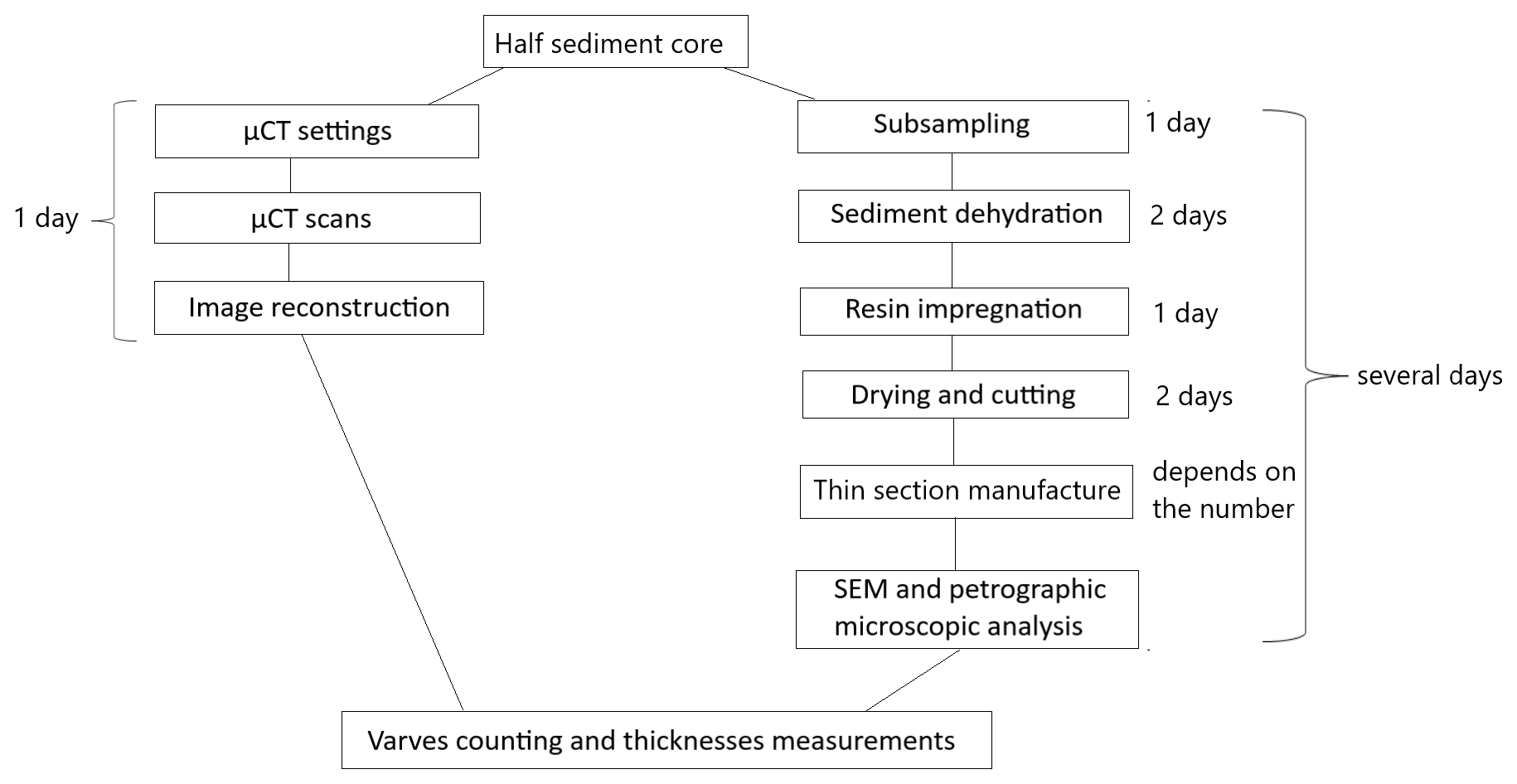
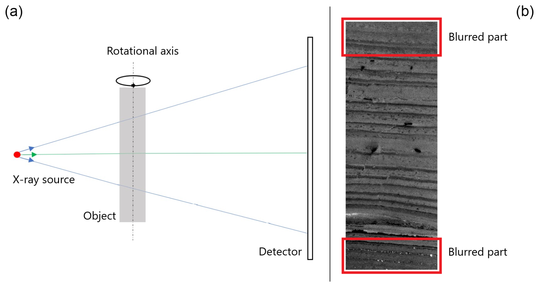
Figure 3 The formation of the beam cone artefact. (a) Presentation in STAMINA mode of the image acquisition mode. The conical X-rays from the source are absorbed by the object, and some of them are transmitted to the detector. The green X-ray follows the shortest distance to reach the detector, while the blue X-rays reach the detector at an angle that causes a mix of information in the vertical direction. (b) Example of a VOI reconstructed with the presence of a beam cone artefact at its boundary parts.

2.3 Experimental setting: µCT acquisition and reconstruction

The scans were made using a TESCAN CoreTOM µCT at INRS-ETE in Quebec City with the Aquila software (version 1.2.1) (Dewanckele et al., 2020). The TESCAN CoreTOM can image complete core samples up to 1.5 m in length, with a spatial resolution of up to 3 µm. This makes it the ideal system for imaging fine laminations such as varves. The half-cores were scanned in a vertical position with a custom-designed acrylic holder, maintaining the half sediment core position during the scans using a foam half-core of the same size. Several instrumental acquisition parameters were tested to identify the best possible configuration to obtain high-resolution images with easily detectable varve boundaries. The best settings were a tube voltage of 140 kV, with an exposure time of 150 ms, an SDD (source detector distance) of 500 mm, and an SOD (source object distance) of 150 mm, resulting in a voxel size of 45 µm. Also, since the µCT uses a polychromatic beam and the different components of the energy spectrum are not uniformly attenuated as they pass through an object, the lower-energy component of the X-ray spectrum is more easily attenuated when it passes through a dense area. This creates brighter voxels during the reconstruction of the images that significantly reduce their quality. These brighter voxels are called beam hardening artefacts (McGuire et al., 2023; Ahmed and Song, 2018). A 1.5 mm thick aluminium filter was therefore used to reduce the impact of this artefact on image quality (Rana et al., 2015; Ay et al., 2013). Smaller subsets of the scans, or volumes of interest (VOIs), were defined along the sediment cores where varves were clearly distinct. Individual VOIs (ca. 30 mm wide, 450 mm thick, 40–60 mm long) (Fig. A2) overlapping each other over 10–20 mm were defined to ensure the continuity of the sedimentary sequence and to deal with the cone beam artefacts (see Fig. 3). Image processing and analysis of these individual VOIs were also made easier for a regular laptop computer. The scanning time depended on the length of the sediment core and varied between 2 h 30 min and 4 h 30 min. Subsequently, these scanned areas were reconstructed with Panthera (TESCAN proprietary software, version 1.5.0.21), with an average reconstruction time of 23 min per reconstructed VOI (Table 1).

The scans were performed using the STAMINA mode (Fig. 3). In other words, projections are acquired over a certain height of the sample while keeping the source and the detector steady as the sample rotates over 360°. Since the beam is conical in STAMINA scans, parts of the VOI outside the central plane of the beam are seen at a specific angle, causing blurred areas at the limit zones of the VOI when imaging horizontal features (Fig. 3) (Laeveren, 2020; Sheppard et al., 2014). Yet, the reconstructed VOIs presented blurred zones at their borders, hereby called the beam cone artefacts, which prevented clear distinction of the limits of the laminae (Laeveren, 2020; Sheppard et al., 2014). However, having overlapping VOIs allowed for easy distinction of laminas that were not visible on a single VOI. This allowed for numerical reconstruction of each sediment core.

2.4 Data analysis

The sediment core images were analysed using the Dragonfly software (version 2022.1). Varve counting and thickness measurements were conducted in two different perpendicular directions, one of which aligns with the thin-section cutting plane. Three counts were performed in each direction on three different cross-sections (Fig. 4a) to ensure three varve counts per direction and compute the average laminae thickness in each direction (Fig. 4a).

Afterwards, the µCT counts were repeated twice in each of the two directions to verify the repeatability of the measurements. For thickness measurements, we observe that deformations tend to widen the varves in the centre of the sediment core. Thus, assuming that the varves are parallel at the time of deposition, we measure the smaller distance between two parallel varve limits to get as close as possible to the initial thickness of the varve before the deformations. The thicknesses were manually measured using the shortest line segment that separates two parallel varve borders perpendicular to them (Fig. 4b). The next step involved creating a thickness variation profile as a function of depth. Each varve was identified by the depth of its top and bottom boundaries, and its thickness was calculated using the depth difference (Fig. A3). Thickness profiles were constructed by summing these values.

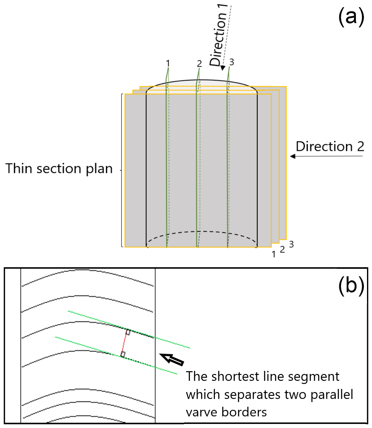
Figure 4 (a) A half sediment core, delimited by black outlines, indicates the directions in which thicknesses are measured. Measurements using µCT are taken in two different directions, with three measurements each. Green outlines indicate the three cross-sections selected in the first direction for counting and thickness measurements of varves, while orange outlines indicate the three cross-sections in the second direction. The thin-section plane corresponds to the first plane of measurements in direction 2. (b) The method used to measure varve thickness involves measuring the length of the shortest line segment between two parallel varve borders.

2.5 Comparing the different thickness measurements

Measurements using the µCT were all conducted along the four sediment cores and were compared with those made on thin sections by Gagnon-Poiré et al. (2021). However, comparisons with the latter were only done at locations where thin sections were sampled and previously analysed. Comparisons with thin sections were thus made throughout cores GL17-04B and GL17-01D and on parts of sediment cores GL17-04C and GL17-05B. Thickness comparisons were made by locating the stratigraphic marker beds to ensure the same varves were compared. It was the average thicknesses of three counts made on µCT direction 1, µCT direction 2, and thin-sections that were compared with each other. This comparison was made using (1) linear regressions, (2) the percentage of the average variation of thicknesses compared to the average value, and (3) the agreement concept (see below). The percentage of the average variation of thicknesses compared to the average is obtained with the following formula:

$$\begin{array}{}\text{(1)}& \begin{array}{rl}& \text{Percentage of average variation of thicknesses}\\ & ={\displaystyle \frac{\text{mean standard deviation}}{\text{mean thickness}}}\times \mathrm{100}.\end{array}\end{array}$$

The study of the differences between thickness measurements on thin sections and those obtained from µCT images was done using the agreement method of Bland and Altman (Altman and Bland, 1983; Grenier et al., 2000; Ranganathan and Aggarwal, 2017). Agreement is a concept that refers to the idea that two or more independent measurements of the same quantity are equivalent (Ranganathan and Aggarwal, 2017). This method compares the observed difference between the values obtained for the same measurement by two different methods. To do so, it calculates the bias and the 95 % confidence interval limits for each measurement and defines the agreement between the two series. The bias (mean of differences) and the limits of agreement represent the deviations of values from one method to another. The difference between the two measurement methods is presented as a function of the mean values obtained with each of the two methods (Fig. A4) (Altman and Bland, 1983; Grenier et al., 2000). For this paper, we define A_i as the thickness measured by method 1 for varve i and B_i as the thickness measured by method 2 for the same varve.

$$\begin{array}{}\text{(2)}& {\displaystyle }\begin{array}{rl}& \text{Difference between the two}\\ & \text{measurement methods for the varve }i=A_i-B_i.\end{array}\text{(3)}& {\displaystyle }\begin{array}{rl}& \text{Mean of the two measurement methods for the varve }\\ & i={\displaystyle \frac{A_i+B_i}{\mathrm{2}}}\end{array}\text{(4)}& {\displaystyle }\text{Bias (or mean of differences)}={\displaystyle \frac{{\sum }_{i=\mathrm{1}}^n(A_i-B_i)}{n}},\end{array}$$

where n is the number of varves.

$$\begin{array}{}\text{(5)}& \begin{array}{rl}& \text{Confidence interval at }\mathrm{95}\mathit{\%}\\ & =\left[\text{bias}-\mathrm{1.96}\times \text{SD; bias}+\mathrm{1.96}\times \text{SD}\right],\end{array}\end{array}$$

where SD is the standard deviation of the differences.

Table 2 Summary of varve counting.

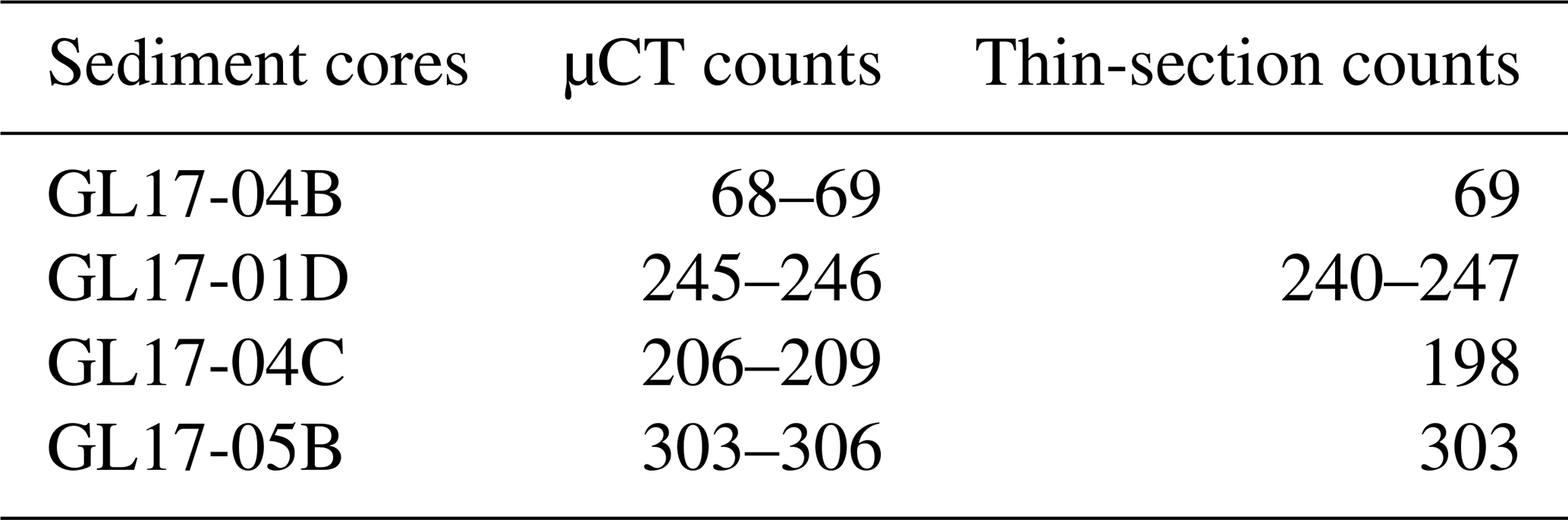
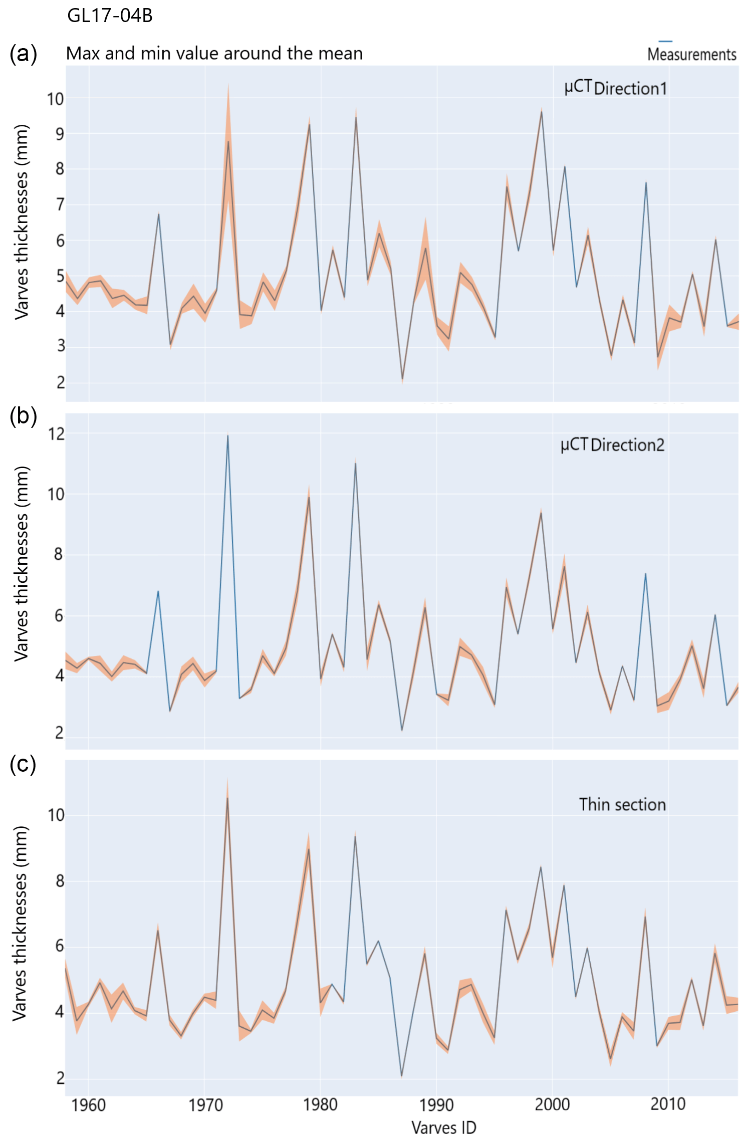
Figure 5 Mean varve thicknesses of the three measurements made in directions 1 (a) and 2 (b) using the µCT and on thin sections (c) for core GL17-04B. The maximum and minimum values around the mean related to the measurements are shown in the orange shaded area, and the varve ID represents the identification of the varve over an interval.

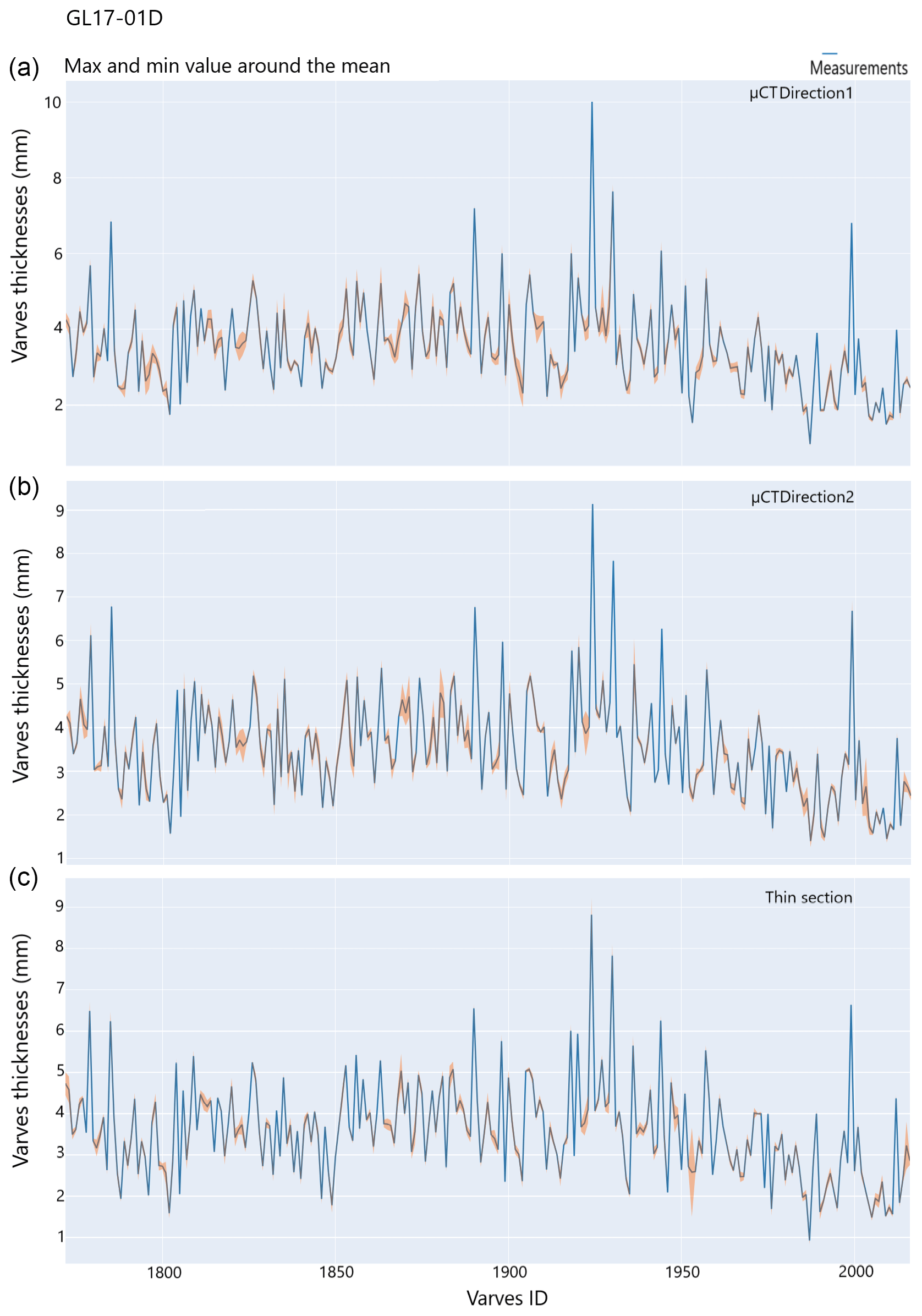
Figure 6 Mean varve thicknesses of the three measurements made in directions 1 (a) and 2 (b) using the µCT and on thin sections (c) for core GL17-01D. The maximum and minimum values around the mean relating to the measurements are shown in the orange shaded area, and the varve ID represents the identification of the varve over an interval.

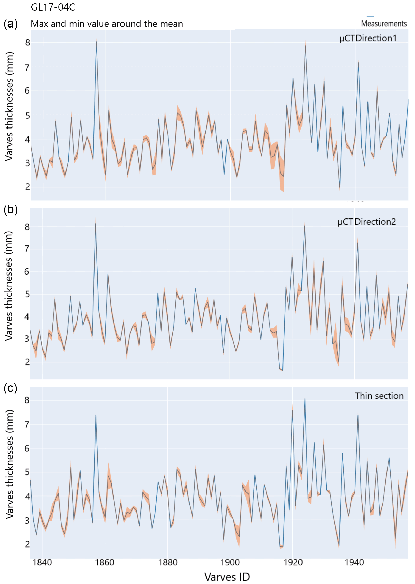
Figure 7 Mean varve thicknesses of the three measurements made in directions 1 (a) and 2 (b) using the µCT and on thin sections (c) for core GL17-04C. The maximum and minimum values around the mean related to the measurements are shown in the orange shaded area, and the varve ID represents the identification of the varve over an interval.

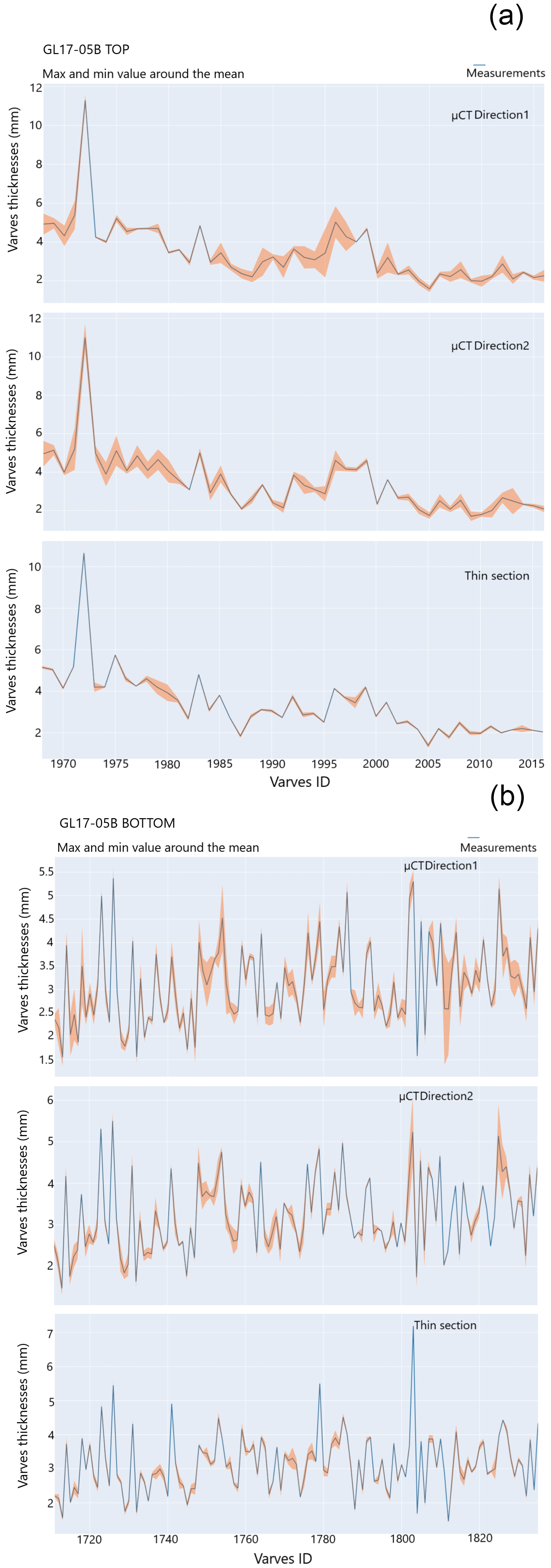
Figure 8 Mean varve thicknesses of the three measurements made in directions 1 (top panels) and 2 (middle panels) using the µCT and on thin sections (lower panels) for core GL17-05B at the top (a) and at the bottom (b). The maximum and minimum values around the mean relating to the measurements are in the orange shaded area, and the varve ID represents the identification of the varve over an interval.

The agreement will be considered good between the two methods when two conditions are fulfilled: there are few points outside the confidence interval and when the points outside the confidence interval are close to the limits of this interval. In this case study, we will define the agreement percentage as the percentage of points outside the confidence interval for each sediment core.

$$\begin{array}{}\text{(6)}& \begin{array}{rl}& \text{Percentage of agreement}\\ & ={\displaystyle \frac{\text{number of points outside the confidence interval}}{\text{number total of points}}}\times \mathrm{100}.\end{array}\end{array}$$

3 Results

3.1 Varve counting

Overall, the number of varves counted with the µCT method is very similar to that of thin sections, except for sediment core GL17-04C, where the number of varves is slightly higher than that of the thin section (Table 2).

3.2 Thickness measurements

The mean varve thicknesses, measured using the µCT and the thin sections in directions 1 and 2, are shown in Figs. 5 to 8. The thickness differences are greater in direction 1 (GL17-04B – Fig. 5, GL17-04C – Fig. 7, and GL17-05B – Fig. 8a–b) than in direction 2. As for GL17-01D (Fig. 6), the measurement differences are less significant and quite similar in both directions. Thickness measurements made on thin sections (Figs. 5–8) are overall less variable than those made on µCT images.

3.3 Repeatability the µCT thicknesses measurements

To evaluate the robustness of the thickness measurements made using the µCT, linear regressions and their determination coefficients R² have been calculated for the measurements made on the same direction. They are all greater than 0.95, with maximum coefficients of 0.996 and 0.997 for the GL17-04B sediment core in directions 1 and 2, respectively. Core GL17-04C shows the next best correlations, and GL17-01D and GL17-05B are those with the weakest but still very high values (Fig. 9).

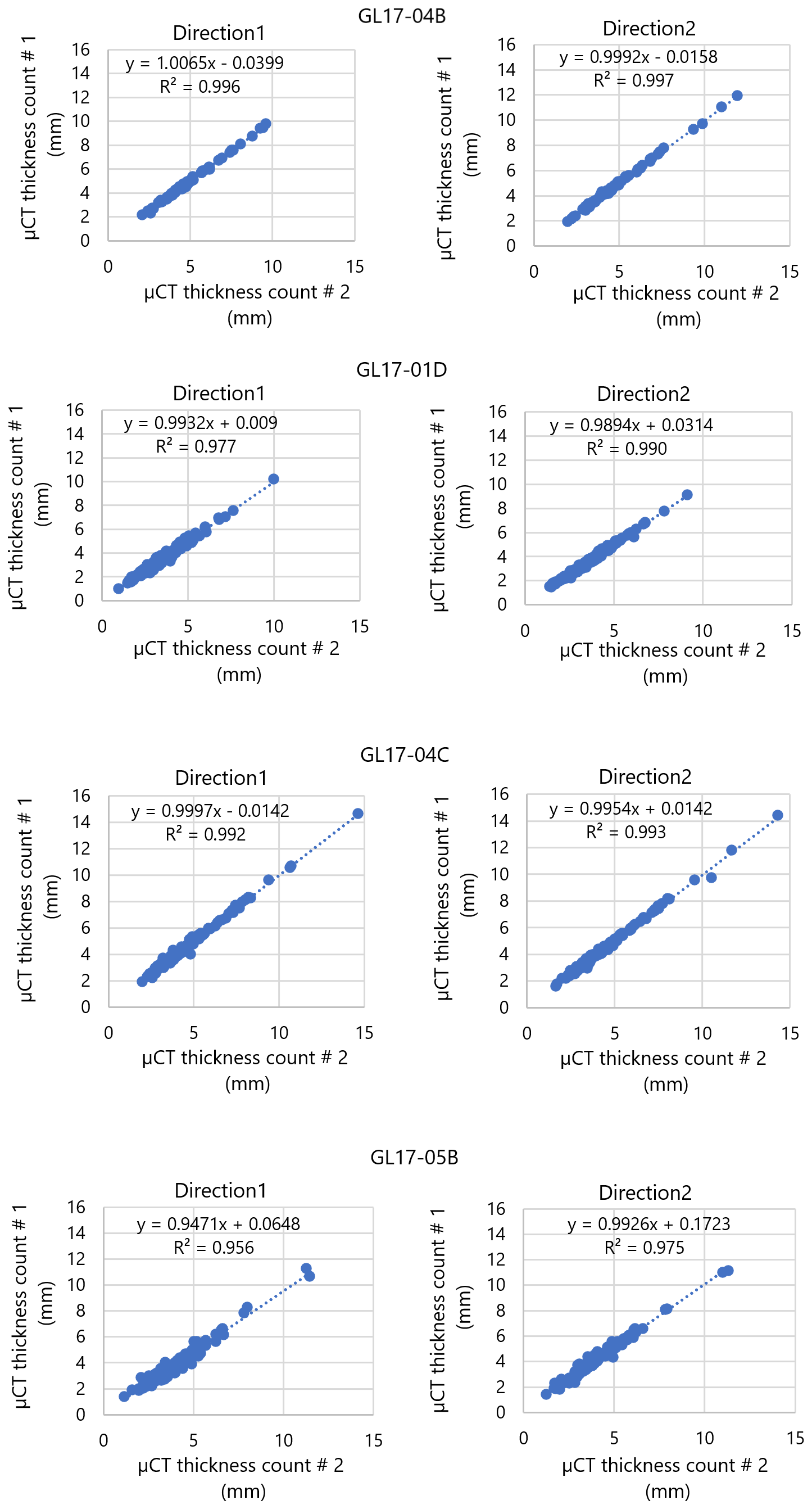
Figure 9 Linear regressions of the mean varve thicknesses measured with µCT between directions 1 and 2 for each sediment core (all measurements are in Appendix B).

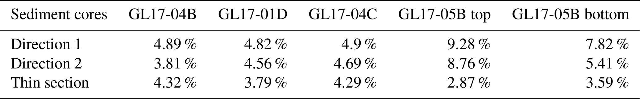
Table 3 Percentage of the average variation of thicknesses compared to the average value.

3.4 Comparison of measurements between µCT and thin sections

The mean thickness measurements with µCT in the two perpendicular directions are compared by linear regression with those obtained by the thin-section method (Fig. 10). The determination coefficients R² vary from 0.768 to 0.828 for minimum correlation and have values between 0.946 and 0.95 for the maximum. In general, the correlations are better in direction 2.

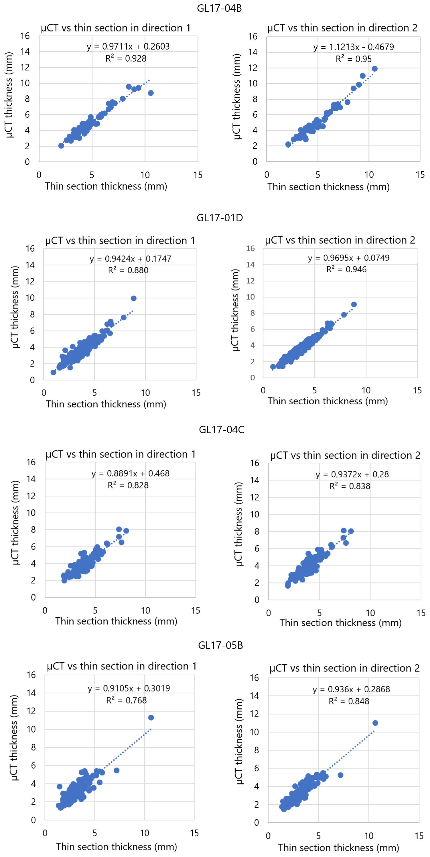
Figure 10 Linear regression between mean thickness measurements made by µCT and thin sections on sediment cores GL17-04B, GL17-01D, GL17-04C, and GL17-05B.

3.5 Percentage of the average variation of thicknesses

Overall, the average percentage variation of thickness compared to the average value is lowest with thin sections, except with GL17-04B. Direction 1 has the highest percentage of thickness variation compared to the second direction. The most important variations are observed with µCT measurements on core GL17-05B, exceeding 5 % compared to other cores. Conversely, with this sediment core, thin sections have the smallest variations in thickness compared to the average (Table 3).

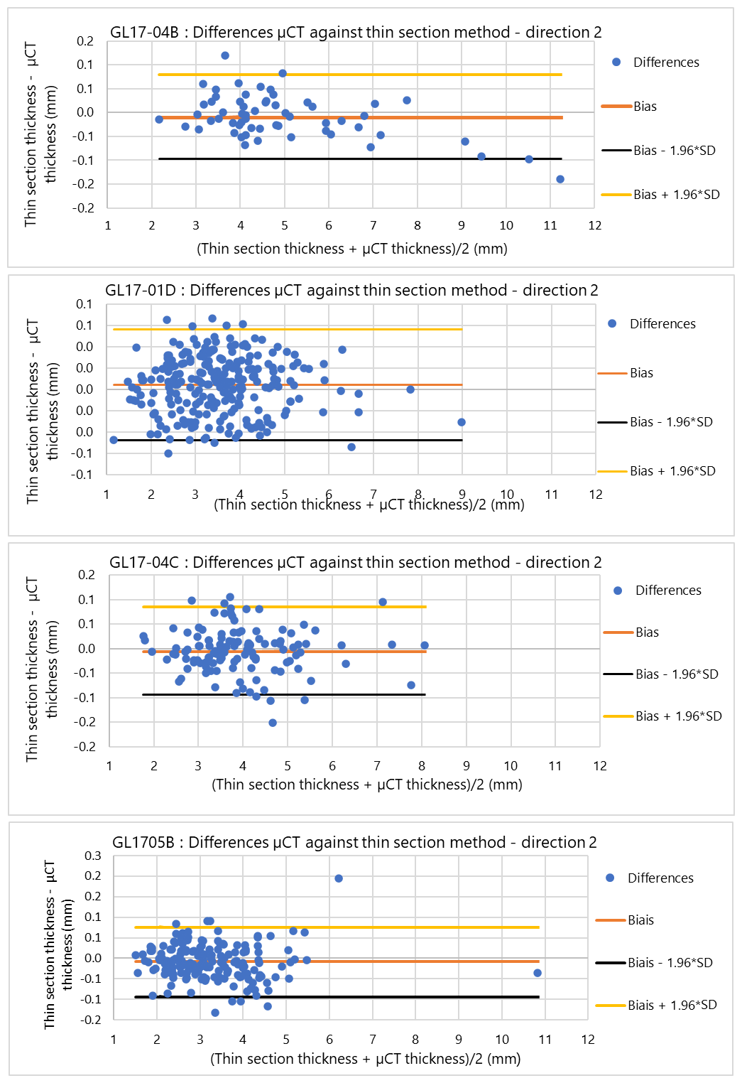
Figure 11 Agreement study in direction 2 between the two methods on sediment cores GL17-04B, GL17-01D, GL17-04C, and GL17-05B. The orange line represents the bias, and the yellow and black lines are the limits of the 95 % confidence interval. Note that the vertical axes do not have similar ranges.

3.6 Agreement study between the two methods

The output of the Bland and Altman agreement method applied on the µCT direction 2 and the thin sections is presented in Fig. 11. The results for direction 1 are presented in Appendix A (Fig. A5).

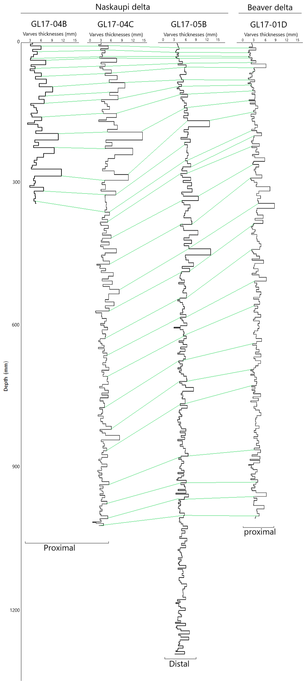
Figure 12 Depth profiles of the four sediment cores. GL17-04B, GL17-04C, and GL17-05B were sampled in front of the Naskaupi River delta. GL17-04B and GL17-04C come from the same drilling site. GL17-01D was sampled from the front of the Beaver River delta. Stratigraphic correlations have been made based on images of sediment cores.

The thickness differences observed with a 95 % confidence interval are as follows: for core GL140B between −0.9615 and 0.7292 mm, with a mean difference (bias) of −0.12 mm; for GL17-01D between −0.4760 and 0.5598 mm, with a mean difference of 0.04 mm; for GL17-04C between −0.9483 and 0.8540 mm, with a mean difference of −0.05 mm; and for GL17-05B between −0.9347 and 0.7721 mm, with a mean difference of −0.08 mm (Fig. 11). Overall, with a 95 % confidence interval, the maximum mean difference obtained is 0.12 mm. The percentage of agreement for GL17-04B, GL17-01D, GL17-04C, and GL17-05B is respectively 96.67 %, 96.73 %, 94.17 %, and 91.95 %.

Table 4 presents a summary of the results obtained.

Table 4 Summary table of results.

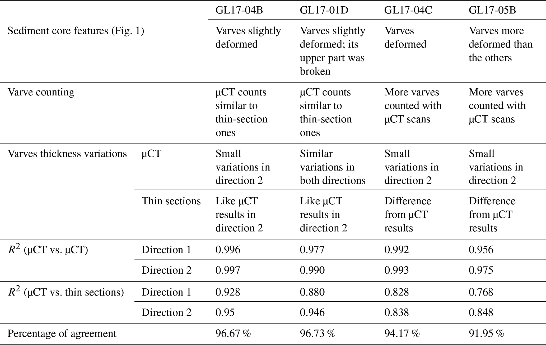
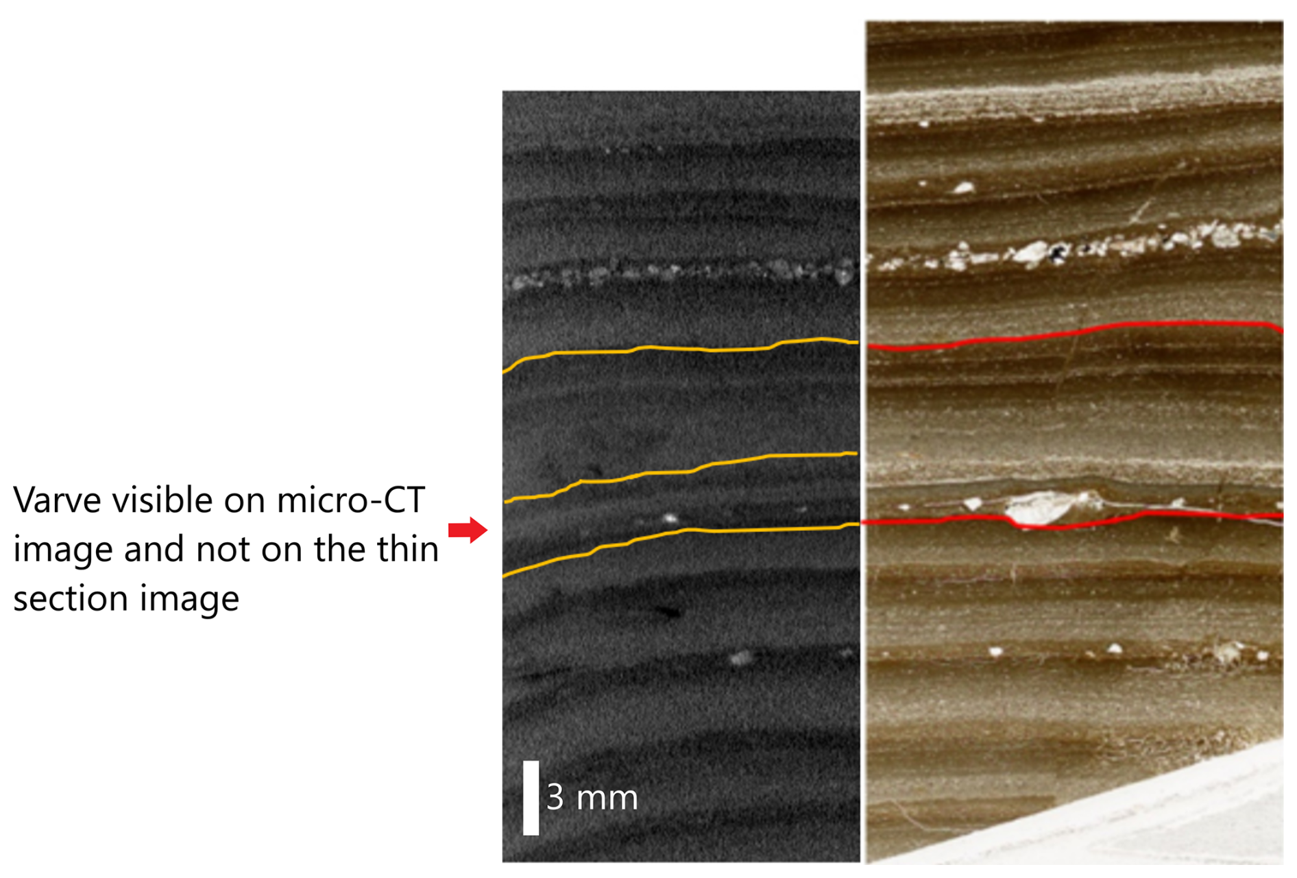
Figure 13 Sediment core GL17-04C shows a lamination that is not visible on the thin-section plane.

3.7 Thicknesses depth profiles

Sediment cores GL17-04C and GL17-04B show almost identical depth profiles in their common parts (Fig. 12). GL17-05B and GL17-01D cores show profiles with a lower amplitude in their thickness variations. Stratigraphic correlations between the cores can be performed.

4 Discussion

4.1 Varve counting

The difference in the number of varves observed when counting with µCT can be explained by several facts. First, 3D analysis with µCT allows access to laminations not visible on the thin-section plane (Fig. 13). Second, there are thin laminations not counted as varves in thin sections, unlike on µCT 3D images (Fig. 14). This is because thin-section observation under a petrographic microscope and the SEM provides more information about lamina features, such as the grain size and grain orientation (Lapointe et al., 2019; Francus, 2006). In this case, the small lamina counted as a varve on the µCT image was considered to be a small event when observed on the thin section because it was not topped with a clay cap, which is the best criterion for accounting for a year of sedimentation (Gagnon-Poiré et al., 2021; Zolitschka et al., 2015). Future work could, however, explore if the grey level values in clay layers could be used to help distinguish the clay cap.

Finally, the presence of deformations in the thin section seems to have an impact on the counting of the varves (Fig. 15). This is one of the great advantages of the 3D view: it allows visual and qualitative analysis of the inside of the sediment core to ensure choosing the best plane for the varved chronology and a wider choice of a region without disturbances.

4.2 Thickness measurements

Direction 1 for the µCT displays larger thickness variations from the mean than direction 2. This can be explained by the fact that this direction presents laminae that are more disturbed. Thus, in the same direction, from one cross-section to another, the measured thicknesses vary. Similarly, GL17-04C and GL17-05B are the sediment cores with the most variations in thickness. These two cores are the most deformed of the four (Fig. 16b and c): a deformation of the varve can induce a simple shift of the measurement point in the same cross-section, leading to an assessable difference in the measured thicknesses. Measuring the thickness of varves at the hinge of a folded boundary is significantly different from measuring the thickness on a perfectly horizontal varve. With the 3D vision of µCT, it is possible to perform scans on larger areas at low resolution in order to select the least distorted areas to perform high-resolution scans (Fig. 17).

The measurements on the thin sections, for their part, present small variations with an average percentage variation of thicknesses less than 5 % (Table 3). This is explained by the fact that with high-resolution images of thin sections, it is possible to see micro-variations in the thickness of the varve.

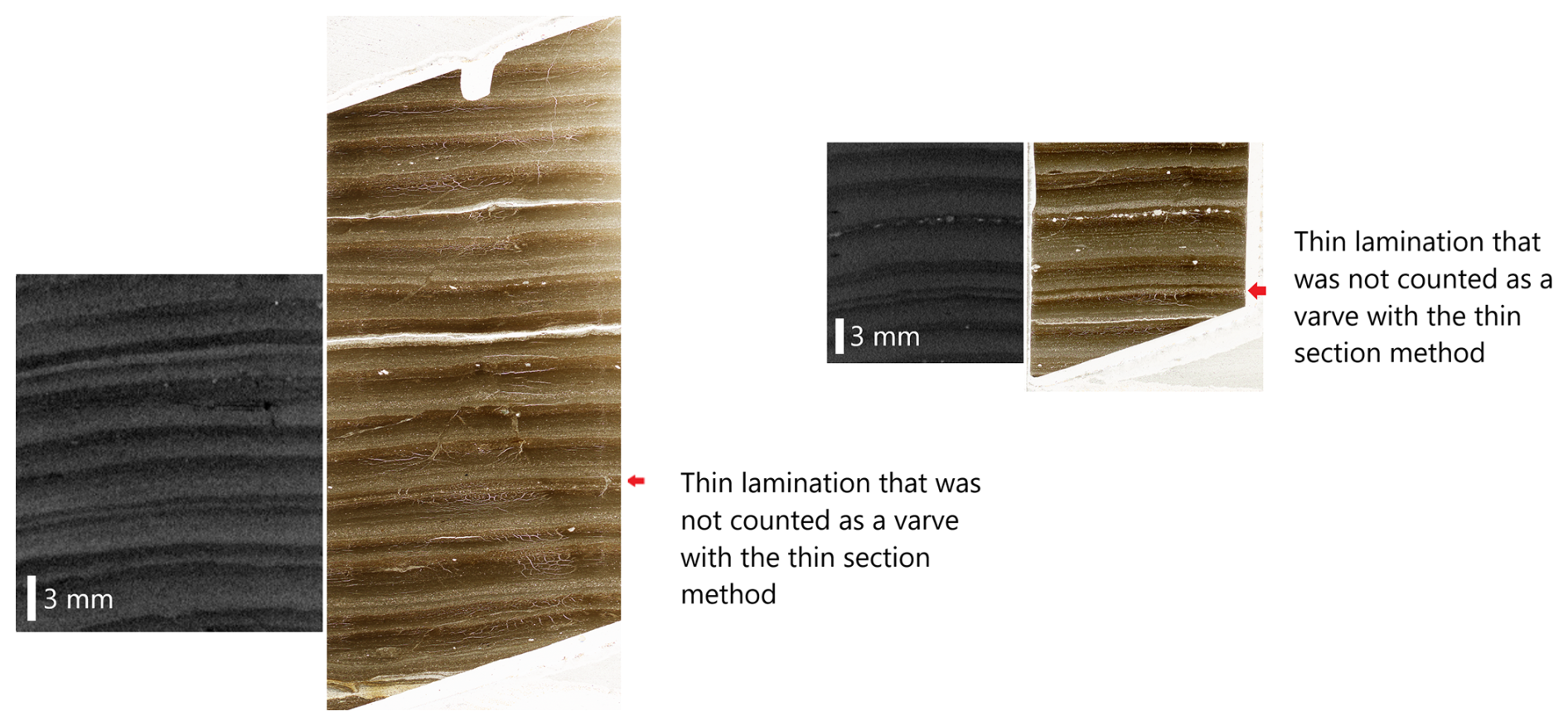
Figure 14 Sediment core GL17-04C shows laminations that are not counted as varves in the thin sections. These laminations are counted as varves with µCT scans, but there is no sedimentological interpretation with µCT scans to confirm that they are actually varves.

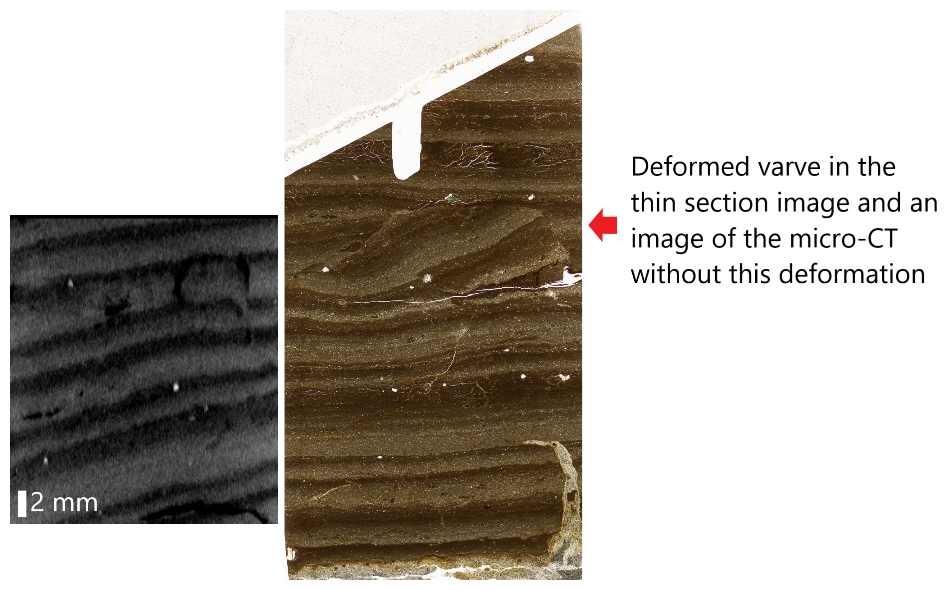
Figure 15 The deformation of varves in the thin-section plane and the corresponding varve with a µCT image in sediment core GL17-05B.

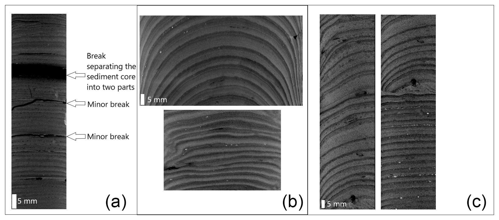
Figure 16 (a) Sediment core GL17-01D has broken parts. (b) Deformations are present in sediment core GL17-05B. (c) Sediment core GL17-04C displays oblique laminations with variable thickness, along with flat and horizontal laminations with constant thicknesses.

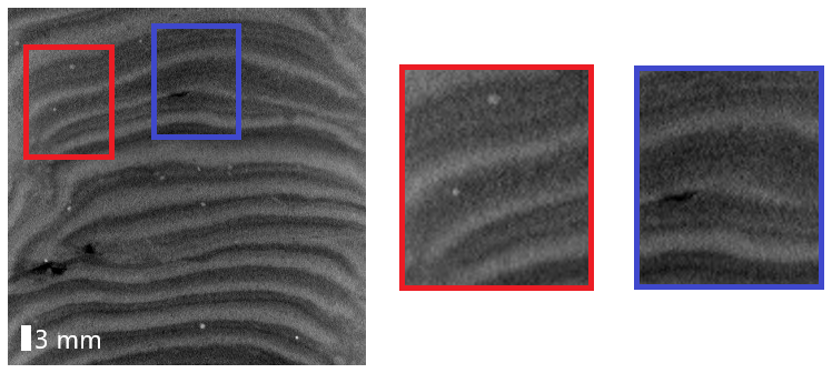
Figure 17 Large VOIs allow you to choose where to do more precise scans within small VOIs. The images with red and purple outlines show how the thickness can vary for the same varve.

Figure 18 Summary of the steps to follow in scanning and reconstructing sediment cores.

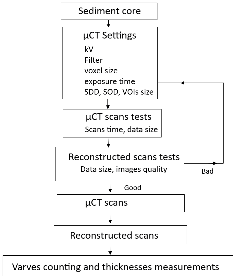
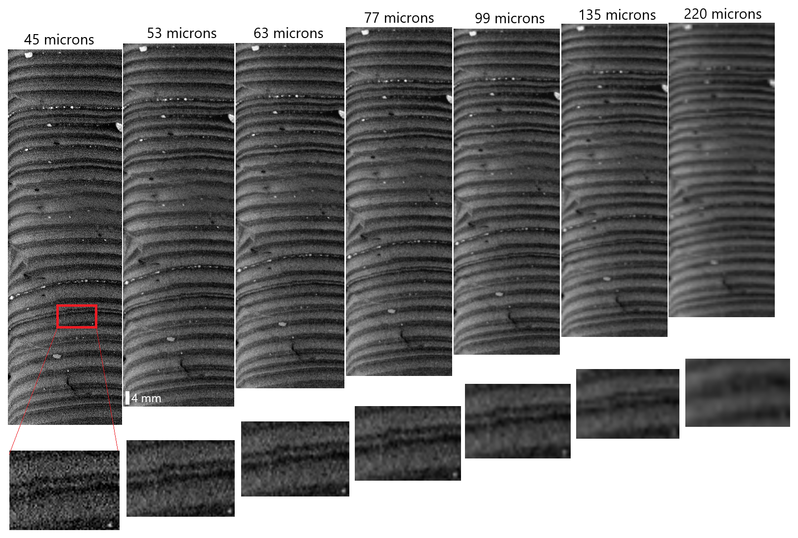
Figure 19 The ability to observe the limits of the smallest stratification depending on the resolution of the µCT images.

4.3 Repeatability of the µCT method

Multiple thickness measurements using µCT show that it is possible to repeat measurements with almost identical values when the laminations are slightly or not deformed. This is the case for the less disturbed core, GL17-04B, that has a correlation coefficient closest to 1 in both directions. It is much easier to reproduce varve thickness measurements almost identically on slightly disturbed sediment cores. More disturbed cores, such as GL17-05B, have lower correlation coefficients, but they are still quite close to 1. Nevertheless, this shows that even slight deformations impact the thickness measurements (Fig. 16).

4.4 Comparison of measurements between µCT and thin sections

Linear regression lines in both directions show slightly different slopes, and the best correlations between µCT and thin-section thickness measurements are obtained in direction 2. This is mainly because direction 2 corresponds to the cutting plane of the sediment core and therefore to the same direction as that of the thin sections. As a result, the points in this direction are significantly better aligned than those in direction 1. As for the agreement study between the two methods, the GL17-04B and GL17-01D sediment cores show the best percentage of agreement above 95 %, followed by GL17-04C with 94.17 % (Table 4). With these sediment cores, the µCT method can be used as a substitute for the thin-section method for these measurements. Additionally, using µCT with deformed sediment cores such as GL17-05B would effectively select the least deformed locations to perform better varve thickness measurements.

4.5 Using µCT to study varved sediment

The use of thin sections is crucial for studying varved sediments (Bendle et al., 2015; Normandeau et al., 2019). Thin sections provide detailed information in one direction, enabling the identification of microstructures and defining sediment nature (Bendle et al., 2015; Brauer and Casanova, 2001; Gagnon-Poiré et al., 2021). Utilizing thin sections to classify and measure varve constituents at short, specific intervals has allowed for high-temporal-resolution environmental reconstructions (Bendle et al., 2015; Brauer and Casanova, 2001; Brauer et al., 2008; Gagnon-Poiré et al., 2021; Lauterbach et al., 2011). However, analysing sediments with thin sections is time-consuming (Normandeau et al., 2019; Francus and Asikainen, 2001; Lotter and Lemcke, 2008).

Measuring varves with µCT can save significant time (Ballo et al., 2023; Emmanouilidis et al., 2020). Indeed, manufacturing thin sections alone takes over 10 d, while µCT allows immediate core scanning without prior preparation. For a 1.5 m sediment core, data acquisition using µCT takes only around 1 d, including parameter testing and scan reconstruction to ensure high-quality images (Fig. 2).

Using µCT would also enhance efficiency, as scanning entire cores prior to sectioning would aid in selecting optimal cutting planes for thin sections, especially in cases of disturbances (Fig. 15). This is a major advantage. Furthermore, for accurate varve chronology and error estimation, conducting multiple counts in different directions is key (Roop et al., 2016; Ballo et al., 2023; Ojala et al., 2012; Zolitschka et al., 2015; Martin-Puertas et al., 2021; Żarczyński et al., 2018). In this study, 12 counts were conducted, including 6 in two perpendicular planes of the sediment core, enhancing understanding of the varve three-dimensional structure.

To more easily detect missing layers or erosional features, it is necessary to steer the counts in parts of the volume that are less affected by disturbances and to make multiple measurements of layers with lateral thickness variations. The µCT also offers the possibility of easily obtaining variations in sediment thicknesses along several sediment cores. This is more practical for performing stratigraphic correlations (Fig. 12).

However, the reconstructed µCT data are large files (Table 1), so it is necessary to have high-capacity computers for their analysis. Careful planning needs to be conducted prior to analysing an entire sequence. For this study, 170 GB was needed for a sediment core 1.5 m long with a resolution of 45 µm. If a higher resolution is needed because laminations are thinner, files will be even larger. For example, to scan GL17-01D at 30 µm, the file size will be 223 GB, so 36 % larger than those at 45 µm. Also, image quality can be affected by artefacts like beam hardening and beam cone artefacts, which can prevent the boundaries of the varves from being clearly distinguished (Laeveren, 2020; Sheppard et al., 2014; Meganck et al., 2009; Davis, 2022). It is important to pay attention to all these details before validating the µCT images (Fig. 18).

A compromise therefore has to be considered to have sufficient resolution to obtain accurate thickness measurements and to have quality images with reduced acquisition and reconstruction times (Du Plessis et al., 2017; Chatzinikolaou and Keklikoglou, 2021; Dewanckele et al., 2020). It is necessary to find the minimum resolution allowing the laminae to be easily distinguished in the shortest possible scanning and reconstruction times. In this case study, it was possible to go well below the resolution of 45 µm (voxel size) obtained for the analysis of the four sediment cores, but this did not provide additional information. Indeed, at 45 µm we can easily distinguish the smallest lamination, which is 0.92 mm thick (∼21 voxels). These limits are visible up to 77 µm (∼12 voxels). Beyond that, the limits of the lamina become blurred (Fig. 19). Thus, to observe varves of 1 mm and to have sharpness of the boundaries, we would need a minimum of about 13 voxels per varve.

5 Conclusion

The well-preserved sequence of thick and undisturbed varves in Grand Lake has allowed us to test the use of µCT to perform varve counts and thickness measurements. Making multiple counts in at least two perpendicular directions allows for obtaining robust varve counts. In addition, with this study it was possible to know the number of voxels needed to observe the limits of varves of millimetric thickness.

The key results are as follows.

• The µCT, with its high resolution, makes it possible to visualize and study varves of millimetre size and below millimetre size.

• The µCT has the potential to reveal the three-dimensional structure of varves and facilitate the detection of missing layers or erosion characteristics.

• The µCT offers the ability to perform multiple layer measurements in multiple directions, resulting in robust thickness measurements in varves with lateral thickness variations.

• In the case of deformed sediment cores, the µCT has the advantage of making it easier to choose the best area for measurements.

Finally, thin sections are still necessary to determine the nature of the varved sedimentary facies and remain essential for contentious cases. However, µCT offers the possibility of no longer making continuous thin sections along a sedimentary sequence for counting and constitutes a powerful tool to improve the quality of the thickness measurements through the access of a 3D view, allowing for choosing the most representative part of the varved record.

Appendix A: Additional images of sediment cores, VOIs shapes, the depth model profile, and information on the agreement study direction 1

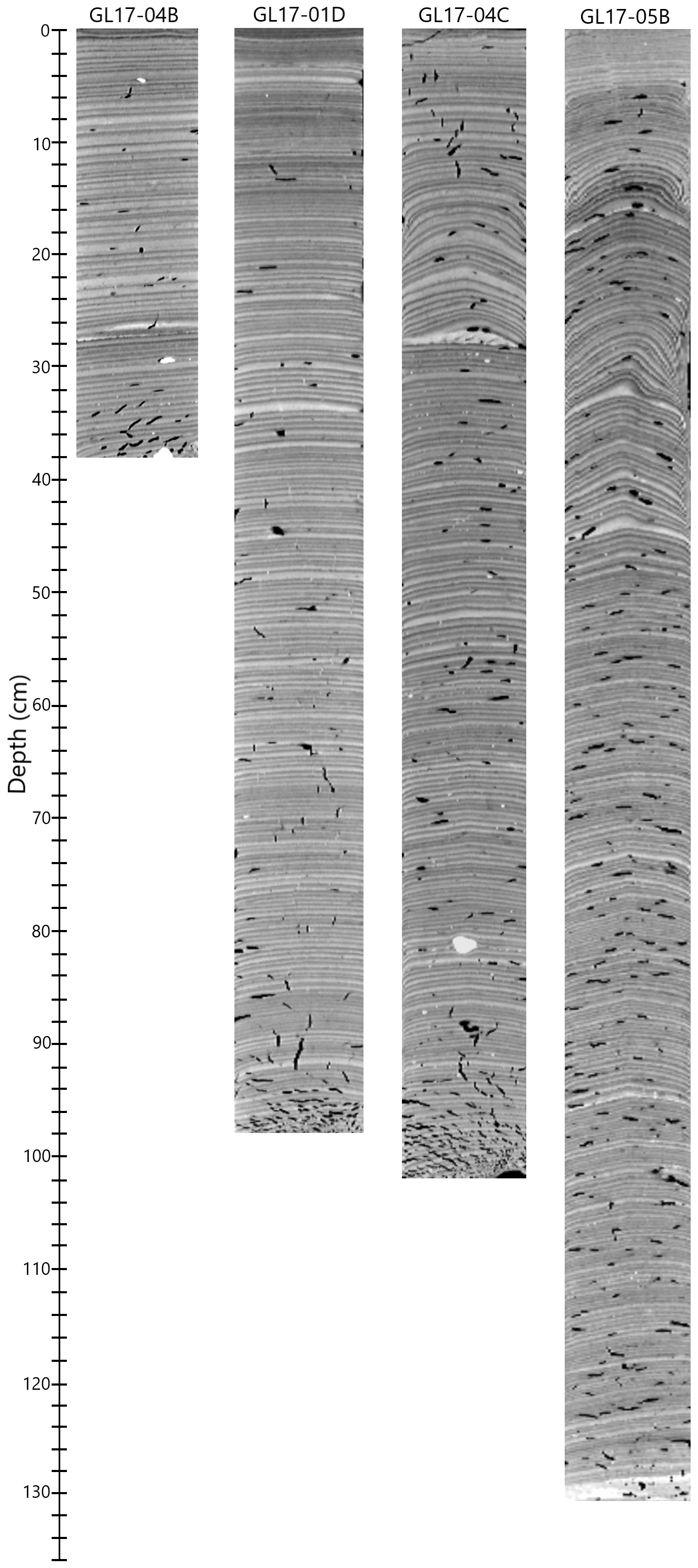
Figure A1 CT scan images of the four sediment cores GL17-04B, GL17-04C, GL17-01D, and GL17-05B used in this study.

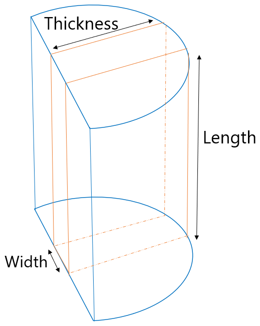
Figure A2 Orange box showing the shape of volumes of interest (VOIs) in the half sediment cores (in blue).

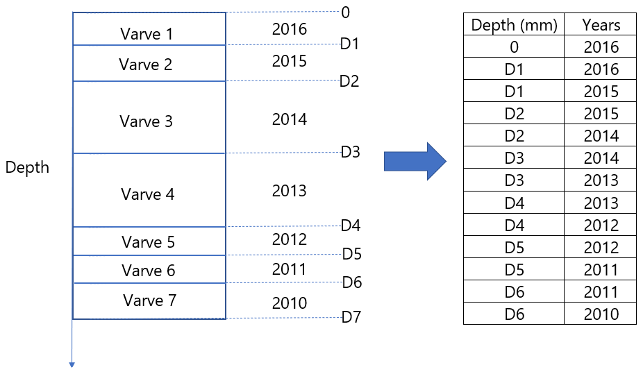
Figure A3 Depth profile calculation model considering that each varve is characterized by two distinct depths.

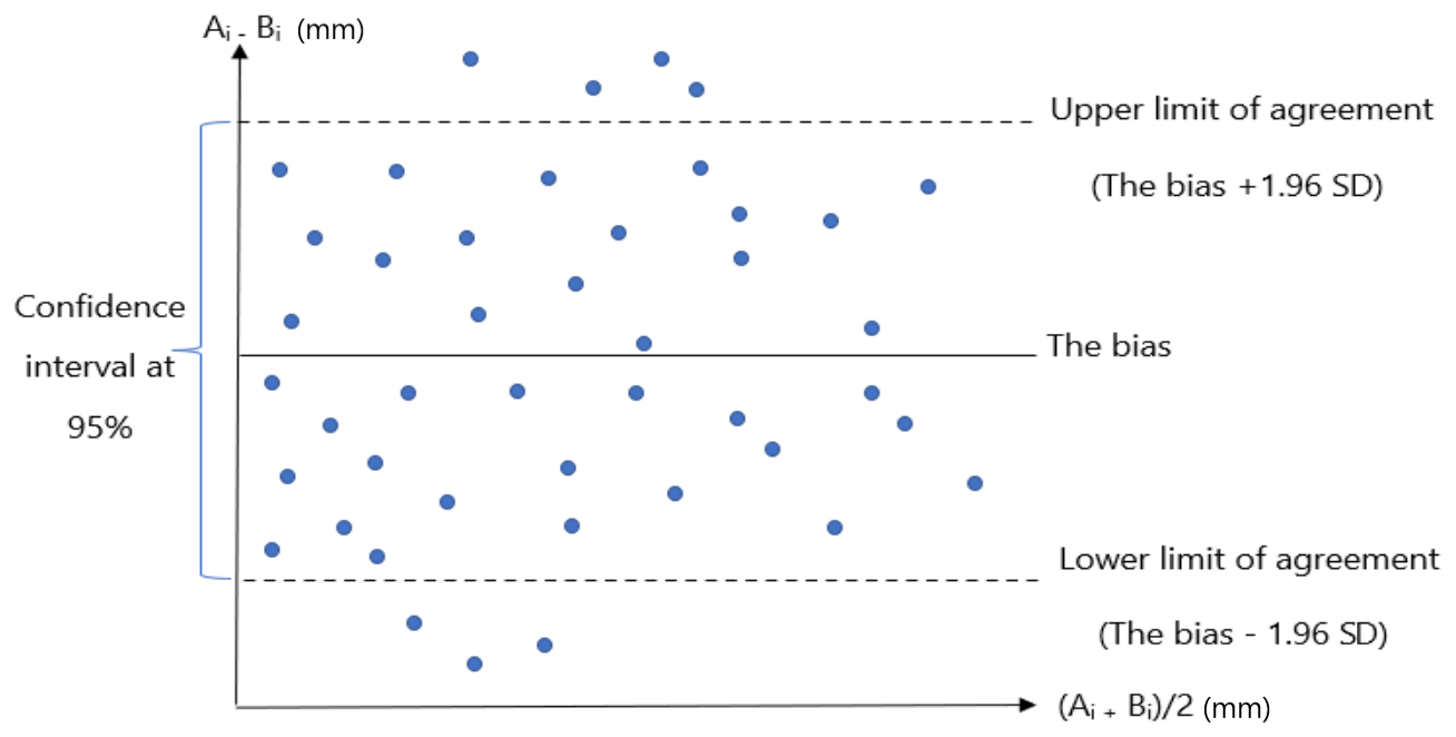
Figure A4 Presentation of the interval in which 95 % of the differences between the two methods are included. Each blue point represents the result of the difference A_i−B_i between two measurements. The upper and lower limits of agreement are the limits of the confidence interval at 95 %. The difference A_i−B_i between the two measurement methods is expressed as a function of the mean values $(A_i-B_i)/\mathrm{2}$ of the results of the two methods.

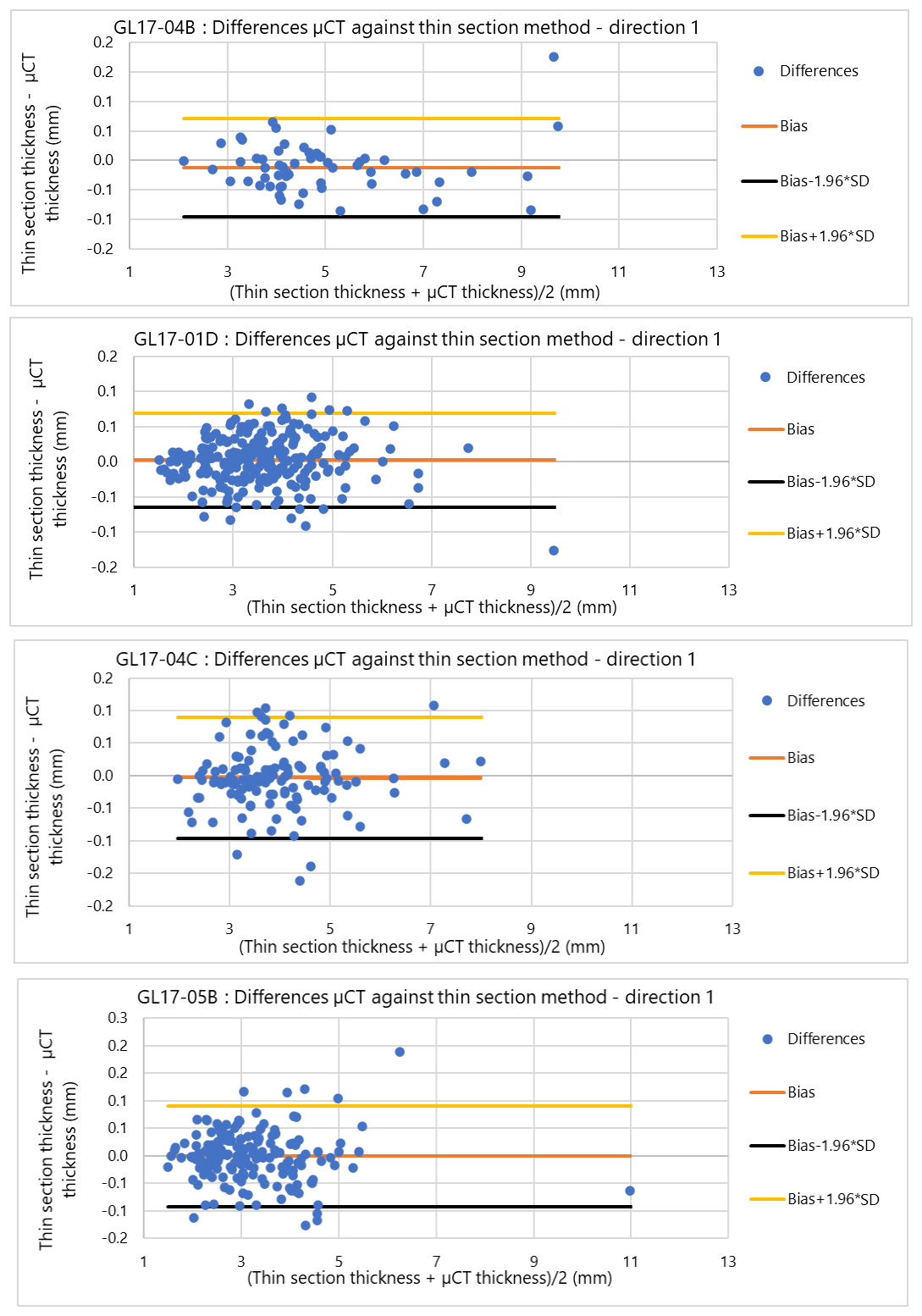
Figure A5 Agreement study in direction 1 for the two methods on sediment cores GL17-04B, GL17-01D, GL17-04C, and GL17-05B. The orange line represents the bias, and the yellow and black lines are the limits of the 95 % confidence interval.

Appendix B: Thickness measurements with µCT and thin sections

Table B1 The thickness measurements with µCT and thin sections.