Extraction of multiple ages from c-axis projected fission tracks

It is generally accepted that the commonly used fission track age equation accurately calculates the cooling age for apatite minerals when the cooling rate is fast. Nevertheless, it is used when the cooling rate is gradual, for example when the age of transition through the partial annealing window is to be estimated. Added age information is here obtained by inclusion of the length distribution of fully included near horizontal tracks. The tendency that the shortest tracks are the oldest ones, and the longest ones are the youngest enables the age dating of a given track by counting the number of shorter tracks, adding one, and dividing by the volumetric track generation rate. The difficulty is that the track length–age relation is blurred by the spread in lengths due to the inherent spread in fission decay energies, crystallographic anisotropy and observational uncertainties. The blurring can be reduced by mathematical deconvolution in which the blurring of tracks in annealing experiments is used. A previously given equation for the oldest track in each histogram column is mathematically further reduced. This paper presents a method where deblurring is first performed by projecting the observed track lengths on the mineral c-axis and then by deblurring using probabilistic least squares inversion. This leads to the extraction of several track ages with deviations for each deconvolved track length histogram. This information may be used to constrain the timing of tectonic events and provide the basis for calculation of past temperature.

1 The fission track equation for age nodes

A commonly used equation to calculate the age of rapid cooling apatite minerals to temperatures below 60 °C is:

$$\begin{array}{}\text{(1)}& t={\displaystyle \frac{\mathrm{1}}{{\mathit{\lambda }}_{\mathrm{D}}}}\ln \left(\mathrm{1}+{\mathit{\lambda }}_{\mathrm{D}}\mathit{\varsigma }g{\displaystyle \frac{{\mathit{\rho }}_{\mathrm{s}}}{{\mathit{\rho }}_{\mathrm{i}}}}{\mathit{\rho }}_{\mathrm{d}}\right),\end{array}$$

where t is the age, λ_D is the total decay constant, ς is a calibration constant in accordance with age standards, g is the geometrical factor (0.5 for pi geometry, 1.0 for 4 pi geometry), ρ_s is the surface track density, ρ_i is the induced fission track density, and ρ_d is the track density in the detector. See Hurford (2019) and Kohn et al. (2024) for a presentation of Eq. (1). The equation is based on earlier development e.g. Fleischer et al. (1975). For example, the age of a volcanic extrusion on the surface is calculated with precision in this way. The essential parameters in the equation are the surface track density, the uranium concentration, and a calibration constant. The equation is also applied to obtain the apparent age for apatite minerals when cooling is gradual through the partial annealing window from 120 to 60 °C (Gleadow, 1981). However, this single age determination can only be regarded as a rough estimate. Jensen and Hansen (2021) showed that several ages can be derived by deconvolution of track length histograms of non- c-axis projected fully included near horizontal fission tracks. The criterion of being horizontal is here that the tracks are in focus at both ends at the same time (Gleadow et al., 1986b; Gleadow et al., 2019).

In this paper the deconvolution method is further developed to apply to c-axis projected tracks. The theoretical foundation is the work by Bertagnolli et al. (1983) and Keil et al. (1987). Their mathematical development concerns the randomly oriented fully included fission track in minerals before they are made visible by etching. These latent tracks are caused by the natural fission of U-238. The latent tracks are generated through time, and their lengths are shortened as a function of time and temperature. In apatite minerals the track lengths are shortened anisotropically contributing to a distribution of lengths. If we for a moment disregard the anisotropy and other blurring effects, it is expected that the oldest tracks are the shortest ones and the more recent tracks are the longest ones. A given track can therefore be aged by integrating the number of random unetched tracks from the longest to the given track and dividing by the track generation rate. This is expressed in the equation (Keil et al., 1987):

$$\begin{array}{}\text{(2)}& \mathit{\tau }\left({\mathit{\lambda }}_{\mathrm{0}}\right)={\displaystyle \frac{\mathrm{1}}{\mathit{\epsilon }}}{\int }_{\mathrm{1}}^{{\mathit{\lambda }}_{\mathrm{0}}}n\left(\mathit{\lambda }\right)\mathrm{d}\mathit{\lambda },\end{array}$$

where τ(λ₀) is the age of a track with a normalized length λ₀, ε is the volumetric track generation rate (tracks s⁻¹ m⁻³), n(λ) is the volumetric density (tracks m⁻³) of tracks with normalized length λ. The integration is performed from the longest tracks (newest) λ=1 to the shorter track (older) λ=λ₀. Unfortunately, it is difficult to see the randomly oriented tracks with a diameter of a few angstroms (Li et al., 2011). Instead, it is therefore practice making them visible in the light microscope by etching (Kohn et al., 2024). To enable length measurement only the near horizontal tracks with a connection to the surface are selected for length measurement. Uranium concentration is also needed. To estimate the ages of etched tracks a mathematical model relating etched tracks to unetched tracks is needed. Due to various biases and uncertainties, the observed track length histogram of etched tracks is blurred. Important factors are (1) the crystallographic biasing (Ketcham, 2003; 2005) causing distribution of track lengths as a function of angle to the c-axis, and (2) the interpreters etching protocol and strategy for track selection (Ketcham, 2003). This means that the relation between histogram columns and the time intervals in which they were generated is non-unique. Fortunately, the blurring is known from artificial annealing experiments and can therefore be deblurred by mathematical deconvolution (Jensen et al., 1992; Donelick, 1988). Probabilistic inversion (Tarantola, 2005) including prior information was implemented for non-c-axis projected tracks (Jensen and Hansen, 2021). After deconvolution the track length histograms were transformed to histograms with a tighter relation between histogram columns and time intervals. The inversion relies on an extended least squares method in which variance and prior information is considered. It is implicitly assumed that the number of tracks in each histogram column is the mean value of a Gaussian distribution with a standard deviation. Because of the use of the least squares method, we only need the mean values and their variances (squared standard deviations) of each histogram column in the equations. Gaussian distribution functions are not needed. The derived deblurred track length histogram was then converted to a time interval histogram. Accumulation of the time interval histogram from the most recent to the older time intervals provided the age of the oldest track of each histogram column, at least those being statistically significant. In this paper the deconvolution technique uses c-axis projected tracks (Donelick et al., 1999). In this way there is a tendency that tracks generated in the same time intervals are brought together in the same histogram columns of c-axis projected tracks. But there is still blurring left which can be deblurred by deconvolution as described here. c-axis projected laboratory annealed tracks are used as the kernel. An approximation in the equations given in Jensen and Hansen (2021) is replaced by a more precise expression. The inversion technique uses the method of least squares which does not exclude negative deconvolved histogram columns. This is of course unrealistic, but the problem can be resolved by the choice of positive priors with small variances but large enough to avoid the priors dominating the deconvolved histograms. That is, the priors are forcing the deconvolved histogram columns to be mainly positive. The weight of the prior can be relaxed by the user of the computer code by increasing the variance of the prior. The mathematical derivations are given in Appendix A. A list of symbols is given in Appendix C. Applications are given in the next Sect. 3.

2 Basics of deconvolution

The ages of tracks in a fission track length histogram are expected to decrease with track length. However, the relation between age and track lengths is not unambiguous due to e.g. crystallographic anisotropy (Ketcham, 2003, 2005), etching protocol and strategy for track selection (Ketcham, 2003). For example, some tracks in a histogram column may originate from a common time interval and the rest from nearby time intervals. This blurring can to some extent be sorted out by mathematical deconvolution. The deconvolution technique was developed in the field of signal analysis and used to filter out noise in telecommunication (Kanasewich, 1975). Deconvolution requires that the probability density of the track length blurring is known (the kernel). This is achieved from laboratory experiments in which apatite minerals are radiated by neutrons in an atomic reactor followed by heating at various temperatures and duration. A track length spread is then observed around the mean track length. The normalized histogram of track lengths is used as the kernel. A similar track length, but smaller, distribution is seen also for c-axis projected tracks.

The principle of simple deconvolution is illustrated in Fig. 1. A synthetic track length histogram is shown in Fig. 1A. The tracks in this histogram are regarded as composed of a weighted sum of normalized track length histograms, Fig. 1B and C, mimicking tracks generated in the laboratory and annealed to two different mean track values. The two normalized histograms are like natural histograms derived from two short time intervals. The synthetic histogram in Fig. 1A is like a natural histogram with a mixture of tracks from two nearby time intervals. It can be decomposed (deconvolved) into a histogram where the tracks in each column originate from the same time interval. It is seen that the synthetic sample, Fig. 1A, can be constructed as the histogram in Fig. 1B times four plus the histogram in Fig. 1C times three. The factors are indicated as columns in Fig. 1E and F and the results of the multiplications are shown in Fig. 1H and I. The sum of these two histograms is shown in Fig. 1G. The choice of factors is correct since the histograms in Fig. 1G and A are equal. Summation of the two columns in Fig. 1E and F is shown in Fig. 1D. This histogram is the deconvolution of the synthetic histogram shown in Fig. 1A. When going the other way, the synthetic histogram is the convolution of the normalized histograms.

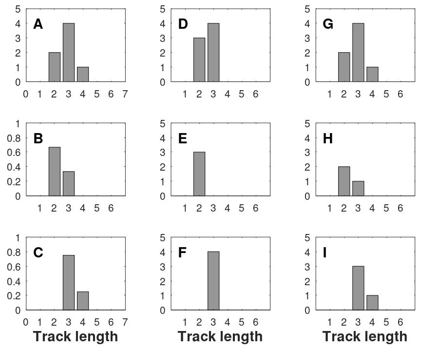
Figure 1 Illustration of deconvolution. (A) A synthetic histogram. (B) A synthetic normalized histogram of tracks generated in a short time interval and then annealed. (C) A histogram like the one in (A) but annealed less. (E, F) Columns representing factors. (H, I) Histograms derived from the histograms in (B) and (C) by multiplication by the factors shown in (E) and (F). (G) Histogram constructed by addition of the histograms in (H) and (I). Histogram (G) is equal to histogram A since the factors (E) and (F) are chosen correctly. (D) This histogram is the deconvolution of histogram (A). It is derived by summation of histograms (E) and (F).

Mathematically the convolution is expressed as the summation of weighted vectors (histograms):

$$\begin{array}{}\text{(3)}& \left[\begin{array}{c}\mathrm{2}\\ \mathrm{4}\\ \mathrm{1}\end{array}\right]=\left[\begin{array}{c}\mathrm{2}/\mathrm{3}\\ \mathrm{1}/\mathrm{3}\\ \mathrm{0}\end{array}\right]\cdot \mathrm{3}+\left[\begin{array}{c}\mathrm{0}\\ \mathrm{3}/\mathrm{4}\\ \mathrm{1}/\mathrm{4}\end{array}\right]\cdot \mathrm{4}\end{array}$$

which is the same as

$$\begin{array}{}\text{(4)}& \left[\begin{array}{c}\mathrm{2}\\ \mathrm{4}\\ \mathrm{1}\end{array}\right]=\left[\begin{array}{cc}\mathrm{2}/\mathrm{3}& \mathrm{0}\\ \mathrm{1}/\mathrm{3}& \mathrm{3}/\mathrm{4}\\ \mathrm{0}& \mathrm{1}/\mathrm{4}\end{array}\right]\left[\begin{array}{c}\mathrm{3}\\ \mathrm{4}\end{array}\right]\end{array}$$

or in general:

$$\begin{array}{}\text{(5)}& \mathit{d}=\mathbf{G}\mathit{m},\end{array}$$

where d is the data vector (for example the synthetic histogram shown in Fig. 1A), G is the smoothing operator with columns of the two normalized histograms, Fig. 1B and C, and m is the model vector (the histogram of factors). The equation expresses a linear relationship between the model m and data d. The rows of G are arranged so that the track length increases down the rows. The degree of annealing of the normalized histograms increases from the left to the right along the columns. The exercise is now to determine an approximation $\stackrel{\mathrm{̃}}{\mathit{m}}$ to the model m given the data d and the operator G:

$$\begin{array}{}\text{(6)}& \mathit{d}=\mathbf{G}\stackrel{\mathrm{̃}}{\mathit{m}}.\end{array}$$

Jensen et al. (1992) used a Monte Carlo type method to solve the equation. The right most column in G was a histogram of mean lengths of tracks derived from Fish Canyon apatite minerals with only slight annealing. The other columns were constructed by shifting this histogram towards lower mean values towards the left in the matrix. Donelick (1988) chose an iterative method where Gaussian functions were used to represent the columns.

In the special case where the number of data and model elements are equal, that is G is squared, $\stackrel{\mathrm{̃}}{\mathit{m}}$ can be calculated directly by matrix inversion:

$$\begin{array}{}\text{(7)}& \stackrel{\mathrm{̃}}{\mathit{m}}={\mathbf{G}}^{-\mathrm{1}}\mathit{d}.\end{array}$$

$\stackrel{\mathrm{̃}}{\mathit{m}}$ is the deconvolution of d. Equation (7) can be generalized to apply for non-squared matrixes: using the least squares method

$$\begin{array}{}\text{(8)}& \stackrel{\mathrm{̃}}{\mathit{m}}=({\mathbf{G}}^{\mathrm{t}}\mathbf{G}{)}^{-\mathrm{1}}{\mathbf{G}}^{\mathrm{t}}\mathit{d},\end{array}$$

where t is the transpose. However, the inversion of the matrix G^tG does not provide realistic solutions when its condition number is large (Bardsley, 2018) and the Eq. (7) does not provide information on the uncertainty of the result. Tarantola (2005) generalized the deconvolution technique to apply to non-squared operators where data and model are not just numbers but probabilistic distributions. This is a valid approach if the relation between model and data is linear or eventually weakly non-linear. Linearity is assured since the number of tracks in a histogram column is a simple summation of tracks originating from various time intervals. Individual elements dⁱ of the data vector d, m^j of the model m, ${\mathit{m}}_{\mathrm{prior}}^j$ of the prior information m_prior are considered being center values of Gaussian distributions. Variances and covariances of data and prior are represented by the matrixes C_D and C_M respectively. The inclusion of prior information diminishes the variance of the expected model $\stackrel{\mathrm{̃}}{\mathit{m}}$ and stabilizes the inversion. In the case where the distributions are Gaussian a direct calculation method was offered by Tarantola (2005):

$$\begin{array}{}\text{(9)}& \stackrel{\mathrm{̃}}{\mathit{m}}={\mathit{m}}_{\mathrm{prior}}+{\left({\mathbf{G}}^{\mathrm{t}}{\mathbf{C}}_{\mathrm{D}}^{-\mathrm{1}}\mathbf{G}+{\mathbf{C}}_{\mathrm{M}}^{-\mathrm{1}}\right)}^{-\mathrm{1}}{\mathbf{G}}^{\mathrm{t}}{\mathbf{C}}_{\mathrm{D}}^{-\mathrm{1}}({\mathit{d}}_{\mathrm{obs}}-\mathbf{G}{\mathit{m}}_{\mathrm{prior}}).\end{array}$$

The data d_obs (the sample histogram) are given with variance (squared standard deviation) and covariance. The result of the deconvolution $\stackrel{\mathrm{̃}}{\mathit{m}}$ is also given with variance and covariance, Eq. (9). $\stackrel{\mathrm{̃}}{\mathit{m}}$ is the posterior (the deblurred track length histogram). m_prior is the prior information on the expected result of the inversion. This information must be independent of the observed data d_obs. In the present paper the priors $m_{\mathrm{prior}}^j$ are selected as default to be equal to the number of measured tracks divided by the number of bins selected for the prior. In this way the prior values are equally distributed over the bins. However, user defined distributions are also allowed. Inclusion of prior information stabilizes the matrix inversions and provides valuable constraints on the result of the inversion. G is the linear operator (matrix) with columns of normalized histograms based on laboratory annealed fission tracks. The t means mathematical transposition. C_D is the variance-covariance matrix of the data. The variances are in the diagonal. The covariance are the off-diagonal elements. The covariance is strong because it is practice counting a specific number of tracks. This means that the variance of the total number of tracks is zero. Increasing the number of tracks of one data element means that other elements must be reduced, indicating strong covariance. This is described by multinomial distribution. The elements of the prior variance-covariance matrix C_M is treated likewise assumed to be multinomial distributed. The variance of each $m_{\mathrm{prior}}^j$ value is chosen to be equal to the number of measured tracks which ensures the possibility that almost all posterior tracks could be placed in a single bin after inversion. The choice for the prior and its variance-covariance ensures that the values of $\stackrel{\mathrm{̃}}{\mathit{m}}$, considered as a histogram, are with mainly positive columns.

The variance-covariance matrix of the posterior $\stackrel{\mathrm{̃}}{\mathit{m}}$ is:

$$\begin{array}{}\text{(10)}& {\stackrel{\mathrm{̃}}{\mathbf{C}}}_{\mathrm{M}}=({\mathbf{G}}^{\mathrm{t}}{\mathbf{C}}_{\mathrm{D}}^{-\mathrm{1}}\mathbf{G}+{\mathbf{C}}_{\mathrm{M}}^{-\mathrm{1}}{)}^{-\mathrm{1}}.\end{array}$$

The variances of the posterior elements are in the matrix diagonal. The covariances are off-diagonal. Time-intervals and variances are calculated directly by an analytical expression based on the posterior $\stackrel{\mathrm{̃}}{\mathit{m}}$ (deblurred histogram) and the variance-covariance ${\stackrel{\mathrm{̃}}{\mathbf{C}}}_{\mathrm{M}}$.

Figures 2 and 3 illustrate input data applied for deconvolution. The vectors in Eq. (A24) are plotted as histograms in Fig. 2 and matrixes are mapped in Fig. 3.

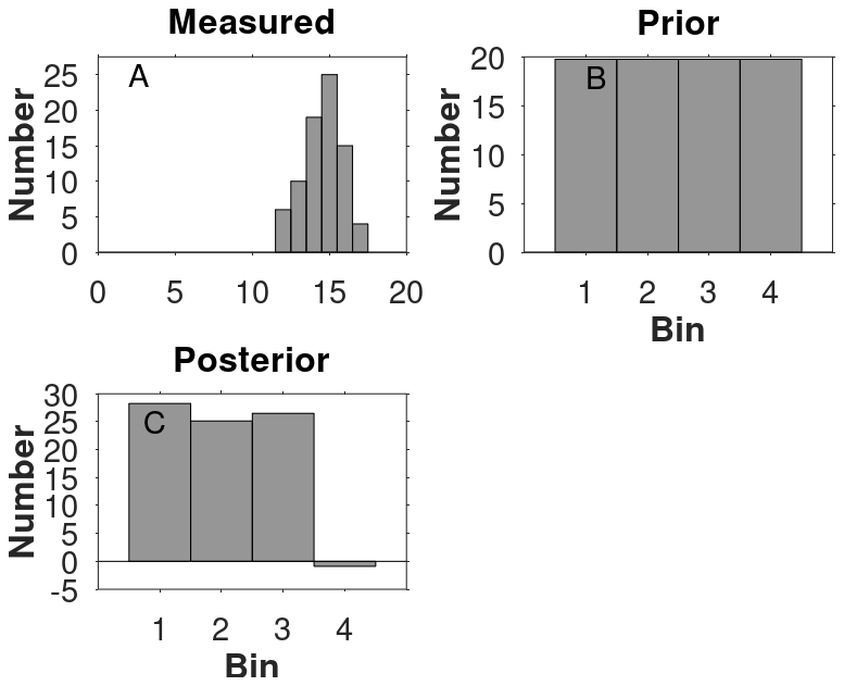
Figure 2 An example of vectors in Eq. (9) shown as histograms. (A) Fission track sample measurements d. (B) Prior information m_prior. The expected number of tracks is distributed equally over the bins. The variance of m_prior is chosen so large that all the posterior tracks could eventually be placed in a single bin but with low probability. (C) The result of the deconvolution is the posterior $\stackrel{\mathrm{̃}}{\mathit{m}}$ calculated by Eq. (9).

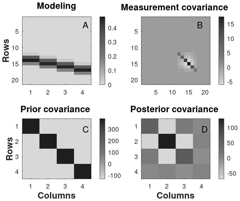
Figure 3 Maps of matrixes in Eq (9). The scale shows the number of tracks. (A) The columns of matrix G are normalized histograms derived by interpolating among track length distributions of radiated samples. The track lengths are increasing with row number. The mean value of the c-axis projected tracks is increasing with column number. (B) Variance-covariance matrix C_D of the data. The diagonal values are the variances of the measurements calculated by Eq. (D1). The off-diagonal values are covariances of the measurements calculated by Eq. (D2). (C) The prior variance-covariance values C_M are calculated by Eqs. (D3) and (D4). (D) The variance-covariance of the deconvolved tracks $\stackrel{\mathrm{̃}}{\mathit{m}}$.

Jensen and Hansen (2021) used Eq. (9) to deblur fission track length histograms based on mean track lengths. The track angles to the mineral c-axis were not considered. Donelick et al. (1999) observed that tracks, longer than approximately 10 µm, generated at the same time after exposition to radiation and after heating, tend to follow an elliptical curve in track length – angle diagrams. Projecting the tracks along an elliptical path to the c-axis assemble tracks generated at the same time. A more complicated track projection method was suggested for shorter tracks described in Donelick et al. (1999). The c-axis projection technique can therefore be considered as deconvolution. However, the projected tracks are still somewhat dispersed needing further deconvolution and relation to time. In this paper the deconvolution technique presented by Jensen and Hansen (2021) is applied to c-axis projected tracks and tested using twenty examples of which five are given below and the rest in the Supplement. It appears that deconvolution enhances the relief of histograms. For example, bimodality becomes clearer even when not evident in the original histograms of c-axis projected tracks. It is also shown here that deconvolution can be helpful identifying erroneous measurements. For example, a histogram may exhibit unrealistically sharp peaks caused by an insufficient number of measured tracks. The reliability of inversion based on Eq. (9) relies heavily on the operator G which is based on measurements of tracks annealed in the laboratory. In this study large databases of track lengths versus angles to the c-axis were provided by Jocelyn Barbarand, personal communication, 2026; Raymond Donelick, personal communication, 2026 based on the work by Carlson et al. (1999), and Ravenhurst et al. (2003). These data were converted to c-axis projected tracks following Donelick et al. (1999).

The mathematical development of the relationship between randomly oriented non-etched tracks and etched horizontal fully included tracks and their relation to time is here reorganized to be smoother compared with the presentation by Jensen and Hansen (2021). The final equation for the oldest tracks in each track length histogram is further mathematically reduced to a simplified version. The equation for the age of the oldest tracks of histogram columns is used to calculate the overall oldest track for twenty samples from Ellesmere Island and Northwest Greenland reported by Spiegel et al. (2023b). The oldest track ages are compared to the apparent ages calculated by Spiegel et al. (2023a). It is not surprising that the oldest track ages are somewhat older than the apparent ages and, in some cases, much older. It is also of interest to compare the ages of the oldest tracks with the ages of peak temperatures experienced by the samples. Ages of the most recent peak temperature above 100 °C for samples reported by Spiegel et al. (2023a) are used for this comparison. The deconvolution technique is also used to identify post-depositional tracks. Several examples are given here. For a given track length histogram, it is important to identify the number and ages of reliable age nodes that can be extracted. The probabilistic inversion approach expressed by Eq. (9) was therefore used to determine age nodes for twenty c-axis projected track histograms derived from Spiegel et al. (2023b).

3 Application of age nodes

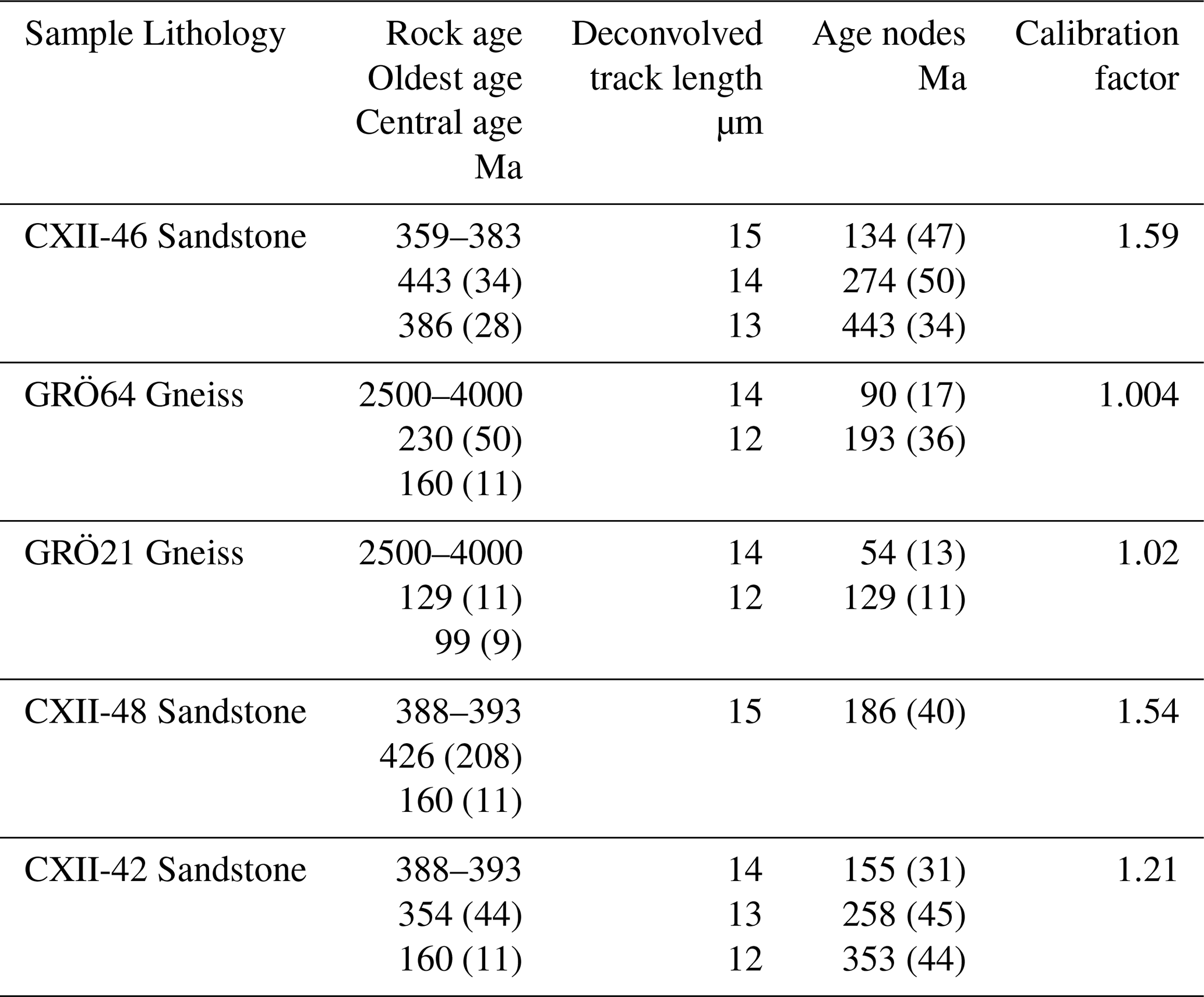
Fission track data from Ellesmere Island and Northwest Greenland (Spiegel et al., 2023a, b) are used to illustrate the calculation of age nodes. Calibrations are performed using histograms of unannealed tracks compared with the corresponding apparent ages. The unannealed histogram is based on artificial tracks at 20 °C (Barbarand et al., 2003) converted to c-axis projected tracks. The calibration constants are given in the Supplement, Table S1.

Calculation of age nodes for the Late Devonian sandstone sample CXII_46. Figure 4A shows the measured c-axis projected fission track length histogram. It is seen that the deconvolved track length histogram (Fig. 4B) is condensed with respect to the track length compared to the original c-axis projected tracks (Fig. 4A). Deconvolution tends to collect the tracks generated in the same time intervals. The columns of the deconvolved track length histogram (Fig. 4B) are converted to equivalent time intervals (Fig. 4C) using

$$\begin{array}{}\text{(11)}& \mathrm{\Delta }{t}^i={\displaystyle \frac{{\mathit{\sigma }}_{\mathrm{s}}}{g{\mathit{\lambda }}_{\mathrm{f}}c{L}_{\mathrm{0}}}}{\displaystyle \frac{{\stackrel{\mathrm{̃}}{\mathfrak{h}}}^i{\sum }_{j=\mathrm{1}}^M\left(\frac{g_j^i}{{\mathit{\kappa }}_j{L}_j}\right)}{{\sum }_{i=\mathrm{1}}^N\left(f\left(l^i\right){\stackrel{\mathrm{̃}}{\mathfrak{h}}}^i{\sum }_{j=\mathrm{1}}^M\left(\frac{g_j^i}{{\mathit{\kappa }}_j{L}_j}\right)\right)}}\end{array}$$

The development of the equation is given in Appendix A. Δtⁱ is the length of time interval i counting from the oldest to the most recent time interval, σ_s is the surface track density, g is the geometrical factor (0.5 for pi geometry, 1.0 for 4 pi geometry), λ_f is the track generation rate, c is the U-238 concentration, L₀ is the initial track length, ${\stackrel{\mathrm{̃}}{\mathfrak{h}}}^i$ is the number of tracks generated in time interval Δtⁱ derived from the deconvolution procedure, ${\sum }_{j=\mathrm{1}}^M$ is summation over all track length bins, $g_j^i$ is the element of row j column i of matrix G. $g_j^i$ is derived from interpolation among track length histograms based on laboratory annealing. ${\mathit{\kappa }}_j=\mathrm{1}/L_j$ for tracks measured in translucent light and κ_j=1 for measurements in reflected light, L_j is the centre of length binning j, ${\sum }_{i=\mathrm{1}}^N$ is summation over the bins of the mean of track lengths, f(lⁱ) is the function describing the relation between the normalized surface track density to the normalized mean track length. Equation (11) is used in the computer program but for future applications it is noted that for tracks measured in translucent light ${\mathit{\kappa }}_j=\mathrm{1}/L_j$ and ${\sum }_{j=\mathrm{1}}^M{g}_j^i=\mathrm{1}$

$$\begin{array}{}\text{(12)}& \mathrm{\Delta }{t}^i={\displaystyle \frac{{\mathit{\sigma }}_{\mathrm{s}}}{g{\mathit{\lambda }}_{\mathrm{f}}c{L}_{\mathrm{0}}}}{\displaystyle \frac{{\stackrel{\mathrm{̃}}{\mathfrak{h}}}^i}{{\sum }_{i=\mathrm{1}}^N\left(f\left(l^i\right){\stackrel{\mathrm{̃}}{\mathfrak{h}}}^i\right)}}.\end{array}$$

The age of the oldest track in each column (Fig. 4C) is derived after cumulation from the longest to the shortest tracks. Three age nodes with non-overlapping deviations are extracted: 134±47, 274±50, and 443±34 Ma (Table 1). The oldest track age, 443±34 Ma, is older than the deposition age of the Late Devonian sandstone (359–383 Ma). This means that the apatite minerals inherit pre-sedimentary tracks. The post-sedimentary columns of the deconvolved histogram (Fig. 4B) were found by identifying the columns with track ages less than the deposition age. In this case they are the three right most track length histogram columns. Post-sedimentary tracks are 70 % of the total number of tracks.

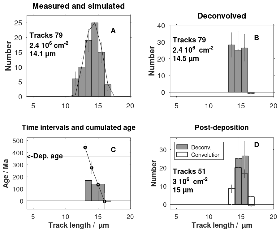
Figure 4 (A) c-axis projected track histogram of a sandstone sample CXII-46, Spiegel et al. (2023b) together with the simulated distribution. (B) Deconvolution of the histogram in (A). (C) Histogram of time intervals and cumulated track ages. The age nodes (black dots) are the y-values plotted as a function of the c-axis projected track lengths and tabulated in Table 1. (D) Deconvolved post-sedimentary tracks and the convolution.

Table 1 Age nodes related to deconvolved track length, calibration factors in Eq. (A30), rock ages (Spiegel et al., 2023b), ages of oldest track using Eq. (A30) with errors (1σ), and fission track central ages (Spiegel et al., 2023b).

Deconvolution tends to enhance bimodality as seen by comparing Fig. 5A and B for sample GRÖ64 (Spiegel et al., 2023b). The age of the oldest track is 230 (50) Ma, Table 1. The bimodality indicates the presence of three levels of maximum temperature: (1) a long period (193–90 Ma) in which the maximum temperature reached the upper part of the partial annealing window (120 to 60 °C) followed by (2) a shorter cooling period where the maximum temperature reached the lower part of the partial annealing window followed by 3) a long period of moderate temperatures below 60 °C until the present.

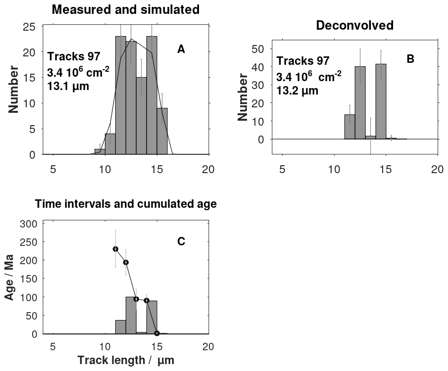
Figure 5 (A) c-axis projected track histogram for sample GRÖ64 (Spiegel et al., 2023b) and the calculated distribution. (B) Deconvolution of the c-axis projected tracks. (C) Histogram of time intervals and cumulated track ages. The age nodes (black dots) are the y-values plotted as a function of the c-axis projected track lengths and tabulated in Table 1.

Figure 6 shows the enhancement of bimodality after the deconvolution of the tracks for sample GRÖ21 (Spiegel et al., 2023b). The measured c-axis projected histogram is broad but non-bimodal. In contrast, the deconvolved histogram shows bimodality.

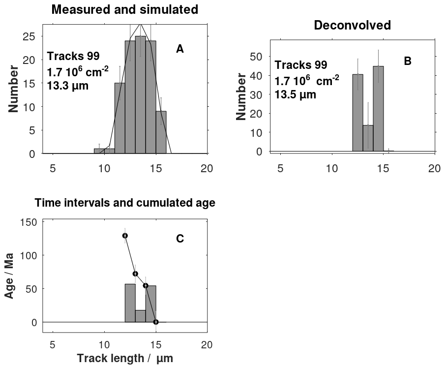
Figure 6 (A) c-axis projected track histogram of the gneiss sample GRÖ21 (Spiegel et al., 2023b) and the calculated distribution. (B) Deconvolution. (C) Histogram of time intervals and cumulated track ages. The age nodes (black dots) are the y-values plotted as a function of the c-axis projected track lengths and tabulated in Table 1.

Figure 7 shows an example with a histogram showing pronounced peaks. Forward calculation based on the deconvolved track length histogram does not mimic the details of the measurements. This is explained by the circumstance that the track length distributions of the kernels do not show sharp peaks. The sample data are therefore insufficiently representing the thermal history of the sample.

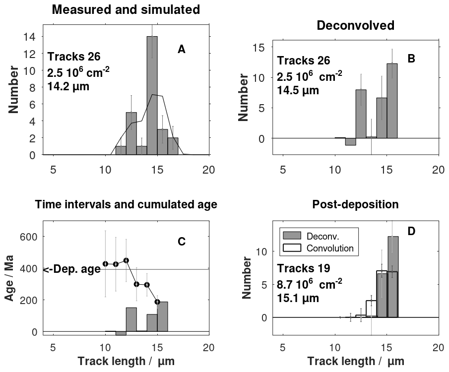
Figure 7 (A) c-axis projected track histogram of the sandstone sample CXII-48 (Spiegel et al., 2023b) showing a poor simulation match to data probably caused by erroneous data. (B) The deconvolution of the histogram shown in (A). (C) Time intervals and cumulated track ages, showing the presence of inherited tracks.

Figure 8 shows a skewed data histogram for a sandstone. The cumulated ages shown in Fig. 8C show the presence of inherited tracks. The c-axis projected tracks longer than 14 µm are post-depositional, Fig. 8D. The convolution (spreading out) of the deconvolved tracks showing the part of the data histogram in Fig. 8A that are expected to be of post-depositional origin.

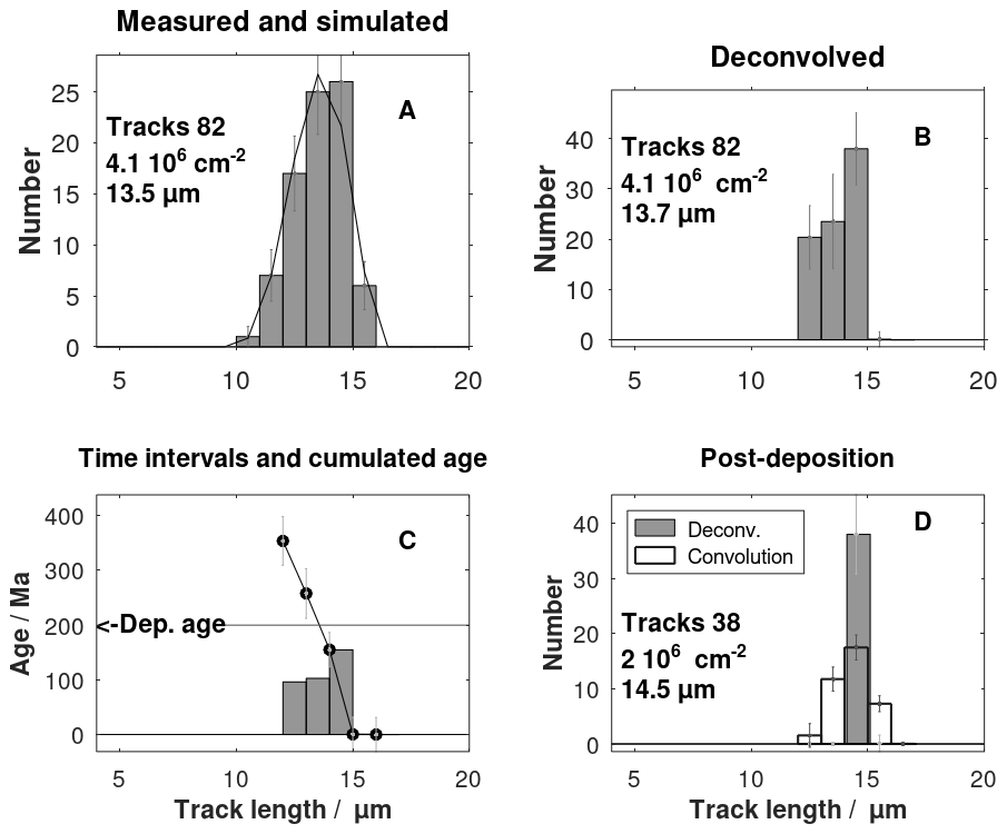
Figure 8 (A) A skewed data c-axis projected track length histogram sample CXII-42 (Spiegel et al., 2023b). (B) The deconvolved track length histogram. (C) The sandstone deposition age is used to extract the post-depositional tracks shown in (D). (D) The deconvolved tracks together with the convolution.

Table S1 shows the calculated age nodes related to the deconvolved track lengths for several samples given by Spiegel et al. (2023b). The computer program written in Octave (Eaton et al., 2020) calculates the oldest track age for each column of the time interval histogram, but only ages with deviations that are not overlapping nearby age deviations are regarded as reliable age nodes. The number of nodes is from two to five with three in mean.

Central ages (Spiegel et al., 2023a) as a function of the calculated oldest ages (this study) show that most central ages are 20 % lower than the oldest ages, Fig. 9. The oldest ages are close to the ages of the last peak temperatures above 100 °C (Spiegel et al., 2023b), however with large deviations.

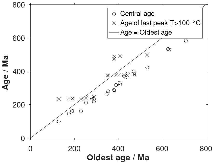
Figure 9 Simulated ages by HeFTy of the last temperature peak with temperatures above 100 °C and central apparent ages (Spiegel et al., 2023b) as a function of the oldest age.

4 Discussion

The least squares inversion method allows negative posterior values (negative histogram columns) which is physically unrealistic. The problem occurs when the physical model is inadequate and the data are mistaken. It is solved by restricting the posterior track length window and choosing positive priors with variances small enough to ensure mainly positive posteriors, but on the other hand so large that the priors do not dominate over the data. The inversion set up applied here assumes individual elements of track length histograms to be normally distributed. In the future, the generalized normal distribution or the log-normal distribution (Tarantola, 2005) may be considered to avoid negative columns. The selection of the normal distribution offers simple equations and direct calculations instead of Monte Carlo type simulations with ten thousand realizations (Gallagher, 2012; Ketcham, 2019). Inversion of matrices like those in Eq. (A24) and (A25) may be non-stable. The stability is tested by calculating the condition numbers for matrixes that are to be inverted. In this case the numbers are small, showing numerical stability. Cholesky factorization is therefore not necessary (Calvetti and Somersalo, 2007). Several factors influence the number of tracks counted for a given track length bin. Important is the bias related to track length. Selection and measurement of track lengths are dependent on effect of light source preferences during observation which are not considered in the present mathematical development.

5 Conclusions

Equations used to calculate multiple age nodes with deviations for apatite fission track length histograms are updated. The equations are based on probabilistic least squares inversion that mitigates the blurring of measured track length histograms. Prior model values are chosen to minimize time-intervals with negative values. The equations were implemented in a computer program (Octave, Eaton et al., 2020) and tested using c-axis projected track data from the Canadian Precambrian Shield. The c-axis projection of the tracks and prior values stabilizes the inversion. The ages of the oldest tracks show conformity with ages of the last temperature peaks above 100 °C, however with large deviations. The ages of the oldest tracks are typically 20 % older than the reported central ages. The age variance shows that two to four age estimates are realistic for c-axis projected track histograms. Bimodality of histograms is enhanced by the deconvolution, promoting the age date estimation of tectonic events. Multiple age node estimates may guide the selection of the age-temperature boxes applied in fission track simulation models.

Appendix A

Jensen and Hansen (2021) discussed direct calculation of multiple age nodes for individual fission track length histograms for non-c-axis projected tracks. The equations are here updated for the use of c-axis projected tracks, which are commonly reported in fission track studies. To deconvolve c-axis projected track histograms, laboratory annealed fission track data are needed. They are derived from laboratory annealing experiments (Carlson et al., 1999; Barbarand et al., 2003; Ravenhurst et al., 2003) and are then c-axis projected following Donelick et al. (1999). The c-axis projection method is based on laboratory annealing experiments by Carlson et al. (1999). The approximation used to derive Eq. (38) in Jensen and Hansen (2021) is here replaced by a more precise expression leading to updated equations.

In a short time-interval Δtⁱ the natural fission of U-238 initially generates a number nⁱ of randomly oriented tracks in the mineral:

$$\begin{array}{}\text{(A1)}& n^i={\mathit{\lambda }}_{\mathrm{f}}c\mathrm{\Delta }{t}^i\mathrm{for}i=\mathrm{1}\mathrm{\dots }N,\end{array}$$

where λ_f is the fission decay frequency c is the U-238 concentration, i numbers the time intervals from the oldest to the most recent interval. Due to the energy dispersion of fission fragments (Jungerman and Wright, 1949), the initial spread of track lengths forms a track length histogram:

$$\begin{array}{}\text{(A2)}& {\mathit{n}}^i=(n_{\mathrm{1}}^i\mathrm{\dots }{n}_j^i\mathrm{\dots }{n}_M^i{)}^{\mathrm{T}},\end{array}$$

where j numbers the track length binning from the shortest to the longest tracks. T indicates mathematical transposition meaning that a row vector is transformed into a column vector.

The initial tracks shorten due to time and the temperature of the mineral. The tracks are further spread in length because of the various orientations relative to the crystal axes. The modified random oriented track length histogram with origin in the time-interval i is

$$\begin{array}{}\text{(A3)}& {\mathit{\nu }}^i=({\mathit{\nu }}_{\mathrm{1}}^i\mathrm{\dots }{\mathit{\nu }}_j^i\mathrm{\dots }{\mathit{\nu }}_M^i{)}^{\mathrm{T}}.\end{array}$$

Consider the time-interval Δtⁱ that produced a number of, not totally annealed, tracks. The total number of these randomly oriented tracks with origin in interval i is

$$\begin{array}{}\text{(A4)}& {\mathit{\nu }}^i={\sum }_{j=\mathrm{1}}^M{\mathit{\nu }}_j^i={\sum }_{j=\mathrm{1}}^M{n}_j^i=n^i={\mathit{\lambda }}_{\mathrm{f}}c\mathrm{\Delta }{t}^i,\end{array}$$

where Eq. (A1) is used.

The randomly oriented tracks are made observable in the light microscope by etching. Only a fraction of the tracks with a connection to the surface is revealed. The histogram of the observable tracks with various orientations is

$$\begin{array}{}\text{(A5)}& {\mathit{e}}^i=(e_{\mathrm{1}}^i\mathrm{\dots }{e}_j^i\mathrm{\dots }{e}_M^i{)}^{\mathrm{T}}.\end{array}$$

It is expected that the number of etched tracks $e_j^i$ is proportional to their lengths: The divisor $\mathrm{1}/L_j$ is therefore appearing in Eq. (A10). On the other hand, short tracks are more likely than long tracks to be accepted as being horizontal. The factor L_j is therefore introduced in Eq. (A8). In this way the tracks measured in translucent light are treated as being unbiased concerning track length:

$$\begin{array}{}\text{(A6)}& {\mathit{e}}^i=K_{\mathrm{1}}(L_{\mathrm{1}}{\mathit{\nu }}_{\mathrm{1}}^i\mathrm{\dots }{L}_j{\mathit{\nu }}_j^i\mathrm{\dots }{L}_M{\mathit{\nu }}_M^i{)}^{\mathrm{T}},\end{array}$$

where L_j is the length corresponding to the histogram column ${\mathit{\nu }}_j^i$ and K₁ is a constant. Fortunately, this constant is cancelled later in the equations.

A subset of horizontal tracks hⁱ is selected from the etched randomly oriented tracks eⁱ for track length measurement:

$$\begin{array}{}\text{(A7)}& {\mathit{h}}^i=(h_{\mathrm{1}}^i\mathrm{\dots }{h}_j^i\mathrm{\dots }{h}_M^i{)}^{\mathrm{T}}.\end{array}$$

This histogram may be length biased compared to the etched tracks eⁱ due to track selection during measurement. Thus, the short tracks are more likely to be accepted as being horizontal than the long ones when measured in translucent light. The randomly oriented tracks ${\mathit{\nu }}_j^i$ are therefore multiplied by ${\mathit{\kappa }}_j=\mathrm{1}/L_j$ to compensate for this bias. See the discussion on selection bias in Jensen et al. (1992). The relation between the selected horizontal tracks and the randomly oriented tracks is therefore

$$\begin{array}{}\text{(A8)}& h_j^i=K_{\mathrm{2}}{\mathit{\kappa }}_j{K}_{\mathrm{1}}{L}_j{\mathit{\nu }}_j^i,\end{array}$$

where K₂ is a constant to be cancelled later. Solving Eq. (A8) for ${\mathit{\nu }}_j^i$:

$$\begin{array}{}\text{(A9)}& {\displaystyle \frac{\mathrm{1}}{K_{\mathrm{2}}{K}_{\mathrm{1}}{\mathit{\kappa }}_j{L}_j}}{h}_j^i={\mathit{\nu }}_j^i\end{array}$$

and after summation on both sides of the equation:

$$\begin{array}{}\text{(A10)}& {\displaystyle \frac{\mathrm{1}}{K_{\mathrm{2}}{K}_{\mathrm{1}}}}{\sum }_{j=\mathrm{1}}^M{\displaystyle \frac{h_j^i}{{\mathit{\kappa }}_j{L}_j}}={\sum }_{j=\mathrm{1}}^M{\mathit{\nu }}_j^i.\end{array}$$

Applying Eq. (A4) yields

$$\begin{array}{}\text{(A11)}& \mathrm{\Delta }{t}^i={\displaystyle \frac{\mathrm{1}}{K_{\mathrm{2}}{K}_{\mathrm{1}}{\mathit{\lambda }}_{\mathrm{f}}c}}{\sum }_{j=\mathrm{1}}^M{\displaystyle \frac{h_j^i}{{\mathit{\kappa }}_j{L}_j}}.\end{array}$$

This equation relates the measured track length histogram hⁱ to the time-interval Δtⁱ in which the tracks were generated. In practice, this tight relationship is disturbed by crossover of tracks from nearby time intervals. It is later shown that this problem can be mediated by a mathematical technique called deconvolution. The problem with the unknown constants is solved by incorporating the surface track density in the equations.

The surface track density σⁱ is related to the mean track length lⁱ of tracks annealed in the laboratory (Green, 1988) after generation in a short time interval Δtⁱ. It is assumed that the experiment mimics the natural track generation and annealing. The normalized surface track density is

$$\begin{array}{}\text{(A12)}& {\displaystyle \frac{{\mathit{\sigma }}^i}{{\mathit{\sigma }}_{\mathrm{0}}^i}}=f\left(l^i\right),\end{array}$$

where lⁱ is the mean track length, f is an empirical relationship, and ${\mathit{\sigma }}_{\mathrm{0}}^i$ is the initial surface track density. It is assumed that ${\mathit{\sigma }}_{\mathrm{0}}^i$ is proportional to the initial track length L₀, the time Δtⁱ that generated the tracks, the track generation rate λ_f, and the Uranium concentration c:

$$\begin{array}{}\text{(A13)}& {\mathit{\sigma }}_{\mathrm{0}}^i=g{\mathit{\lambda }}_{\mathrm{f}}c{L}_{\mathrm{0}}\mathrm{\Delta }{t}^i.\end{array}$$

where g is the geometrical factor (0.5 for 2 pi geometry, 1.0 for 4 pi geometry). Combining Eqs. (A12) and (A13):

$$\begin{array}{}\text{(A14)}& {\mathit{\sigma }}^i=g{\mathit{\lambda }}_{\mathrm{f}}c{L}_{\mathrm{0}}f\left(l^i\right)\mathrm{\Delta }{t}^i.\end{array}$$

The function f(lⁱ) is valid for c-axis projected tracks (Appendix B). Inserting the expression for Δtⁱ, Eq. (A11), leads to the surface track density corresponding to time interval Δtⁱ.

$$\begin{array}{}\text{(A15)}& {\mathit{\sigma }}^i={\displaystyle \frac{g{L}_{\mathrm{0}}}{K_{\mathrm{2}}{K}_{\mathrm{1}}}}f\left(l^i\right){\sum }_{j=\mathrm{1}}^M\left({\displaystyle \frac{h_j^i}{{\mathit{\kappa }}_j{L}_j}}\right).\end{array}$$

The total surface density σ_s caused by the track generation in all time intervals is then:

$$\begin{array}{}\text{(A16)}& {\mathit{\sigma }}_{\mathrm{s}}={\sum }_{i=\mathrm{1}}^N{\mathit{\sigma }}^i={\displaystyle \frac{g{L}_{\mathrm{0}}}{K_{\mathrm{2}}{K}_{\mathrm{1}}}}{\sum }_{i=\mathrm{1}}^N\left(f\left(l^i\right){\sum }_{j=\mathrm{1}}^M\left({\displaystyle \frac{h_j^i}{{\mathit{\kappa }}_j{L}_j}}\right)\right).\end{array}$$

The ratio is

$$\begin{array}{}\text{(A17)}& {\displaystyle \frac{{\mathit{\sigma }}^i}{{\mathit{\sigma }}_{\mathrm{s}}}}={\displaystyle \frac{f\left(l^i\right){\sum }_{j=\mathrm{1}}^M\left(\frac{h_j^i}{{\mathit{\kappa }}_j{L}_j}\right)}{{\sum }_{i=\mathrm{1}}^N\left(f\left(l^i\right){\sum }_{j=\mathrm{1}}^M\left(\frac{h_j^i}{{\mathit{\kappa }}_j{L}_j}\right)\right)}}.\end{array}$$

Taking advantage of Eqs. (A14) and (A17) lead to

$$\begin{array}{}\text{(A18)}& \mathrm{\Delta }{t}^i={\displaystyle \frac{{\mathit{\sigma }}_{\mathrm{s}}}{g{\mathit{\lambda }}_{\mathrm{f}}c{L}_{\mathrm{0}}}}{\displaystyle \frac{{\sum }_{j=\mathrm{1}}^M\left(\frac{h_j^i}{{\mathit{\kappa }}_j{L}_j}\right)}{{\sum }_{i=\mathrm{1}}^N\left(f\left(l^i\right){\sum }_{j=\mathrm{1}}^M\left(\frac{h_j^i}{{\mathit{\kappa }}_j{L}_j}\right)\right)}}.\end{array}$$

The age of the beginning of time-interval p is obtained by summation of all time intervals from interval p to N (the most recent):

$$\begin{array}{}\text{(A19)}& t_p={\sum }_{i=p}^N\mathrm{\Delta }{t}^i={\displaystyle \frac{{\mathit{\sigma }}_{\mathrm{s}}}{g{\mathit{\lambda }}_{f}c{L}_{\mathrm{0}}}}{\displaystyle \frac{{\sum }_{i=p}^N{\sum }_{j=\mathrm{1}}^M\left(\frac{h_j^i}{{\mathit{\kappa }}_j{L}_j}\right)}{{\sum }_{i=\mathrm{1}}^N\left(f\left(l^i\right){\sum }_{j=\mathrm{1}}^M\left(\frac{h_j^i}{{\mathit{\kappa }}_j{L}_j}\right)\right)}}.\end{array}$$

The corresponding surface track density is after summation using Eq. (A17)

$$\begin{array}{}\text{(A20)}& {\mathit{\sigma }}_p={\mathit{\sigma }}_{\mathrm{s}}{\displaystyle \frac{{\sum }_{i=p}^N\left(f\left(l^i\right){\sum }_{j=\mathrm{1}}^M\left(\frac{h_j^i}{{\mathit{\kappa }}_j{L}_j}\right)\right)}{{\sum }_{i=\mathrm{1}}^N\left(f\left(l^i\right){\sum }_{j=\mathrm{1}}^M\left(\frac{h_j^i}{{\mathit{\kappa }}_j{L}_j}\right)\right)}}.\end{array}$$

${\mathit{h}}^i=(h_{\mathrm{1}}^i\mathrm{\dots }{h}_j^i\mathrm{\dots }{h}_M^i{)}^{\mathrm{T}}$is the histogram of tracks generated in the time-interval Δtⁱ. Although most of the tracks in the elements $h_j^i$ of length lⁱ are generated in the time interval Δtⁱ there will also be tracks from neighboring time intervals due to track length mixing. However, it was shown in Jensen and Hansen (2021) that the order can be restored, to some extent, by mathematical deconvolution. The idea is that the measured track length histogram is considered as a weighted sum of histograms of tracks generated in short time interval. These histograms, with various degrees of annealing, are derived from laboratory annealing experiments:

$$\begin{array}{}\text{(A21)}& \begin{array}{rl}& \left[\begin{array}{c}\begin{array}{c}{h}^{\mathrm{1}}\\ \mathrm{⋮}\end{array}\\ \mathrm{⋮}\\ \begin{array}{c}{h}^i\\ \begin{array}{c}\mathrm{⋮}\\ h^M\end{array}\end{array}\end{array}\right]={\mathfrak{h}}^{\mathrm{1}}\left[\begin{array}{c}\begin{array}{c}{g}_{\mathrm{1}}^{\mathrm{1}}\\ \mathrm{⋮}\end{array}\\ \mathrm{⋮}\\ \begin{array}{c}{g}_j^{\mathrm{1}}\\ \begin{array}{c}\mathrm{⋮}\\ g_M^{\mathrm{1}}\end{array}\end{array}\end{array}\right]\\ & +\mathrm{\dots }{\mathfrak{h}}^i\left[\begin{array}{c}\begin{array}{c}{g}_{\mathrm{1}}^i\\ \mathrm{⋮}\end{array}\\ \mathrm{⋮}\\ \begin{array}{c}{g}_j^i\\ \begin{array}{c}\mathrm{⋮}\\ g_M^i\end{array}\end{array}\end{array}\right]+\mathrm{\dots }{\mathfrak{h}}^n\left[\begin{array}{c}\begin{array}{c}{g}_{\mathrm{1}}^N\\ \mathrm{⋮}\end{array}\\ \mathrm{⋮}\\ \begin{array}{c}{g}_j^n\\ \begin{array}{c}\mathrm{⋮}\\ g_M^N\end{array}\end{array}\end{array}\right]\end{array}\end{array}$$

or

$$\begin{array}{}\text{(A22)}& \begin{array}{rl}& \left[\begin{array}{c}\begin{array}{c}{h}^{\mathrm{1}}\\ \mathrm{⋮}\end{array}\\ \mathrm{⋮}\\ \begin{array}{c}{h}^i\\ \begin{array}{c}\mathrm{⋮}\\ h^M\end{array}\end{array}\end{array}\right]\\ & =\left[\begin{array}{ccc}{g}_{\mathrm{1}}^{\mathrm{1}}& \mathrm{\dots }& g_{\mathrm{1}}^i\\ \mathrm{⋮}& \mathrm{⋮}& \mathrm{⋮}\\ \begin{array}{c}\mathrm{⋮}\\ g_j^{\mathrm{1}}\\ \begin{array}{c}\mathrm{⋮}\\ g_M^{\mathrm{1}}\end{array}\end{array}& \begin{array}{c}\mathrm{⋮}\\ \mathrm{\dots }\\ \begin{array}{c}\mathrm{⋮}\\ \mathrm{\dots }\end{array}\end{array}& \begin{array}{c}\mathrm{⋮}\\ g_j^i\\ \begin{array}{c}\mathrm{⋮}\\ g_M^i\end{array}\end{array}\end{array}\begin{array}{cc}\mathrm{\dots }& g_{\mathrm{1}}^N\\ \mathrm{⋮}& \mathrm{⋮}\\ \begin{array}{c}\mathrm{⋮}\\ \mathrm{\dots }\\ \begin{array}{c}\mathrm{⋮}\\ \mathrm{\dots }\end{array}\end{array}& \begin{array}{c}\mathrm{⋮}\\ g_j^N\\ \begin{array}{c}\mathrm{⋮}\\ g_M^N\end{array}\end{array}\end{array}\right]\\ & \cdot \left[\begin{array}{c}{\mathfrak{h}}^{\mathrm{1}}\\ \mathrm{⋮}\\ \begin{array}{c}{\mathfrak{h}}^i\\ \mathrm{⋮}\\ {\mathfrak{h}}^N\end{array}\end{array}\right]\end{array}\end{array}$$

or simply:

$$\begin{array}{}\text{(A23)}& \mathit{h}=\mathbf{G}\mathfrak{h},\end{array}$$

where the vector h is the measured histogram, G a matrix with columns of normalized histograms derived from laboratory annealing and chosen so that their mean track length lⁱ is binned according with the columns of the matrix. 𝔥 is the vector of weights. The number of tracks in a histogram column is regarded as the mean values of a Gaussian distribution. This is the case for histograms h and 𝔥 in Eq. (A24) and the histograms of each column of the matrix G. The squared standard deviations (1σ) of the Gaussians are implemented in the diagonals of C_H and C_P in Eq. (A24). Each histogram column in G is derived from neutron radiation in a short time-interval with following annealing. The columns of G are here based on c-axis projections of the laboratory annealed tracks described by Carlson et al. (1999), Barbarand et al. (2003) and Ravenhurst et al. (2003). The histogram 𝔥 is the deconvolution of the sample histogram h. In this process h is deblurred (Bardsley, 2018) with respect to track length mixing. Appendix C provides a list of various vectors and matrices.

The unknown 𝔥 in Eq. (A23) is solved using least squares probabilistic inversion (Tarantola, 2005) which includes prior information 𝔥_prior:

$$\begin{array}{}\text{(A24)}& \stackrel{\mathrm{̃}}{\mathfrak{h}}={\mathfrak{h}}_{\mathrm{prior}}+{\left({\mathbf{G}}^{\mathrm{T}}{\mathbf{C}}_{\mathrm{H}}^{-\mathrm{1}}\mathbf{G}+{\mathbf{C}}_{\mathrm{P}}^{-\mathrm{1}}\right)}^{-\mathrm{1}}{\mathbf{G}}^{\mathrm{T}}{\mathbf{C}}_{\mathrm{H}}^{-\mathrm{1}}(\mathit{h}-\mathbf{G}{\mathfrak{h}}_{\mathrm{prior}}),\end{array}$$

where $\stackrel{\mathrm{̃}}{\mathfrak{h}}$ is the posterior (the deblurred histogram) which replaces $h_j^i$ in Eqs. (A19) and (A20). C_H and C_P are data and prior variance-covariance matrixes.

The least squares inversion scheme Eq. (A24) allows calculated negative posterior values in conflicts with the fact that the numbers of tracks are positive. To minimize the problem h_prior is chosen to be with positive elements. In most cases, we do not have much information on the prior. Its elements are therefore chosen to be equal and with sum equal to the number of measured tracks. Their variances (the diagonal of C_P) are chosen to be so large that all posterior tracks are allowed in a single posterior element. See Appendix D for discussion of prior values.

The variance-covariance of the deblurred histogram is calculated according to Tarantola (2005):

$$\begin{array}{}\text{(A25)}& {\stackrel{\mathrm{̃}}{\mathbf{C}}}_{\mathrm{P}}={\left({\mathbf{G}}^{\mathrm{T}}{\mathbf{C}}_{\mathrm{H}}^{-\mathrm{1}}\mathbf{G}+{\mathbf{C}}_{\mathrm{P}}^{-\mathrm{1}}\right)}^{-\mathrm{1}}.\end{array}$$

The approximation $\stackrel{\mathrm{̃}}{h}$ to the data histogram h is forwardly calculated based on the posterior (deblurred) histogram $\stackrel{\mathrm{̃}}{\mathfrak{h}}$:

$$\begin{array}{}\text{(A26)}& \stackrel{\mathrm{̃}}{\mathit{h}}=\mathbf{G}\stackrel{\mathrm{̃}}{\mathfrak{h}},\end{array}$$

where $\stackrel{\mathrm{̃}}{\mathfrak{h}}=({\stackrel{\mathrm{̃}}{h}}^{\mathrm{1}}\mathrm{\dots }{\stackrel{\mathrm{̃}}{h}}^i\mathrm{\dots }{\stackrel{\mathrm{̃}}{h}}^N{)}^{\mathrm{T}}$.

The approximation ${\stackrel{\mathrm{̃}}{\mathit{h}}}^i$ to the observed tracks with origin in the time interval Δtⁱ is derived from Eq. (A26):

$$\begin{array}{}\text{(A27)}& \begin{array}{rl}& \left[\begin{array}{ccc}{g}_{\mathrm{1}}^{\mathrm{1}}& \mathrm{\dots }& g_{\mathrm{1}}^i\\ \mathrm{⋮}& \mathrm{⋮}& \mathrm{⋮}\\ \begin{array}{c}\mathrm{⋮}\\ g_j^{\mathrm{1}}\\ \begin{array}{c}\mathrm{⋮}\\ g_M^{\mathrm{1}}\end{array}\end{array}& \begin{array}{c}\mathrm{⋮}\\ \mathrm{\dots }\\ \begin{array}{c}\mathrm{⋮}\\ \mathrm{\dots }\end{array}\end{array}& \begin{array}{c}\mathrm{⋮}\\ g_j^i\\ \begin{array}{c}\mathrm{⋮}\\ g_M^i\end{array}\end{array}\end{array}\begin{array}{cc}\mathrm{\dots }& g_{\mathrm{1}}^N\\ \mathrm{⋮}& \mathrm{⋮}\\ \begin{array}{c}\mathrm{⋮}\\ \mathrm{\dots }\\ \begin{array}{c}\mathrm{⋮}\\ \mathrm{\dots }\end{array}\end{array}& \begin{array}{c}\mathrm{⋮}\\ g_j^N\\ \begin{array}{c}\mathrm{⋮}\\ g_M^N\end{array}\end{array}\end{array}\right]\\ & \cdot \left[\begin{array}{c}\mathrm{0}\\ \mathrm{⋮}\\ \begin{array}{c}{\mathfrak{h}}^i\\ \mathrm{⋮}\\ \mathrm{0}\end{array}\end{array}\right]={\stackrel{\mathrm{̃}}{\mathfrak{h}}}^i,\end{array}\end{array}$$

where an element of ${\stackrel{\mathrm{̃}}{\mathit{h}}}^i$ is

$$\begin{array}{}\text{(A28)}& {\stackrel{\mathrm{̃}}{h}}_j^i=g_j^i{h}^i\end{array}$$

which replaces $h_j^i$ in Eqs. (A18) and (A19). This improves the corresponding equation given in Jensen and Hansen (2021). The final expressions for the age of the beginning of interval Δt^p is

$$\begin{array}{}\text{(A29)}& t_p={\sum }_{i=p}^N\mathrm{\Delta }{t}^i={\displaystyle \frac{{\mathit{\sigma }}_{\mathrm{s}}}{g{\mathit{\lambda }}_{f}c{L}_{\mathrm{0}}}}{\displaystyle \frac{{\sum }_{i=p}^N{\stackrel{\mathrm{̃}}{\mathfrak{h}}}^i{\sum }_{j=\mathrm{1}}^M\left(\frac{g_j^i}{{\mathit{\kappa }}_j{L}_j}\right)}{{\sum }_{i=\mathrm{1}}^N\left(f\left(l^i\right){\stackrel{\mathrm{̃}}{\mathfrak{h}}}^i{\sum }_{j=\mathrm{1}}^M\left(\frac{g_j^i}{{\mathit{\kappa }}_j{L}_j}\right)\right)}}.\end{array}$$

Considering the radioactive exponential decay the final expression for the age of the oldest track in column p is obtained:

$$\begin{array}{}\text{(A30)}& t_p={\displaystyle \frac{\mathit{\eta }}{{\mathit{\lambda }}_{\mathrm{D}}}}\ln \left(\mathrm{1}+{\displaystyle \frac{{\mathit{\sigma }}_{\mathrm{s}}{\mathit{\lambda }}_{\mathrm{D}}}{g{\mathit{\lambda }}_{f}c{L}_{\mathrm{0}}}}{\displaystyle \frac{{\sum }_{i=p}^N\left({\stackrel{\mathrm{̃}}{\mathfrak{h}}}^i{\sum }_{j=\mathrm{1}}^M\right(\frac{g_j^i}{{\mathit{\kappa }}_j{L}_j}\left)\right)}{{\sum }_{i=\mathrm{1}}^N\left(f\left(l^i\right){\stackrel{\mathrm{̃}}{\mathfrak{h}}}^i{\sum }_{j=\mathrm{1}}^M\left(\frac{g_j^i}{{\mathit{\kappa }}_j{L}_j}\right)\right)}}\right),\end{array}$$

where t_p is the expected age of the oldest track in column p of the deblurred track histogram $\stackrel{\mathrm{̃}}{\mathfrak{h}}=({\stackrel{\mathrm{̃}}{\mathfrak{h}}}^{\mathrm{1}},{\stackrel{\mathrm{̃}}{\mathfrak{h}}}^{\mathrm{2}},\mathrm{\dots }{\stackrel{\mathrm{̃}}{\mathfrak{h}}}^i,\mathrm{\dots }{\stackrel{\mathrm{̃}}{\mathfrak{h}}}^N{)}^{\mathrm{T}}$. The columns are counted from small to long track lengths, η is a calibration constant, λ_D is the total decay constant, σ_s is the surface track density, $g=\mathrm{1}/\mathrm{2}$ is the geometric factor, λ_f is the U-238 fission decay constant, c is the U-238 concentration, L₀ is the mean track length of unannealed tracks, ${\stackrel{\mathrm{̃}}{h}}^i$ is an element of the deconvolved track length histogram, $g_j^i$ is an element of the interpolated laboratory annealed track length histogram, ${\mathit{g}}^i=(g_{\mathrm{1}}^i\mathrm{\dots }{g}_j^i\mathrm{\dots }{g}_M^i{)}^{\mathrm{T}}$, κ_j compensates for the track selection bias, ${\mathit{\kappa }}_j=\mathrm{1}/L_j$ for tracks measured in translucent light, κ_j=1 for tracks measured in reflected light, L_j is the track length of the tracks related to $g_j^i$, f(lⁱ) is the normalized surface track density of ${\stackrel{\mathrm{̃}}{\mathfrak{h}}}^i$ with mean track length lⁱ (the track length bin of ${\stackrel{\mathrm{̃}}{\mathfrak{h}}}^i$ (Appendix B), N is the number of bins of the deconvolved track length histogram, M is the number of bins of the observed track length histogram.

The calibration constant η is in practice derived by calculating the oldest age using Eq. (A30) for a deconvolved unannealed track length histogram age and matching it to the apparent fission track age obtained by the usual fission track age equation. In this way we take advantage of the calibration used in the commonly used age equation. The radiated sample (Barbarand et al., 2003), kept at 20 °C, is used in the calibrations.

Application of Eqs. (A28) and (A20) leads to the updated expression for the surface track density

$$\begin{array}{}\text{(A31)}& {\mathit{\sigma }}_p={\mathit{\sigma }}_{\mathrm{s}}{\displaystyle \frac{{\sum }_{i=p}^N\left(f\left(l^i\right){\stackrel{\mathrm{̃}}{\mathfrak{h}}}^i{\sum }_{j=\mathrm{1}}^M\left(\frac{g_j^i}{{\mathit{\kappa }}_j{L}_j}\right)\right)}{{\sum }_{i=\mathrm{1}}^N\left(f\left(l^i\right){\stackrel{\mathrm{̃}}{\mathfrak{h}}}^i{\sum }_{j=\mathrm{1}}^M\left(\frac{g_j^i}{{\mathit{\kappa }}_j{L}_j}\right)\right)}}.\end{array}$$

Appendix B

The normalized surface track density is related to the normalized track length and described for c-axis projected tracks by Raymond Donelick (personal communication, 2026). The normalized surface track density, Fig. B1, is:

$$\begin{array}{}\text{(B1)}& {\mathit{\sigma }}^i/{\mathit{\sigma }}_{\mathrm{0}}^i=f\left(l^i\right),\end{array}$$

where σⁱ is the observed surface track density and ${\mathit{\sigma }}_{\mathrm{0}}^i$ is the initial surface track density. lⁱ is the mean track length of observed c-axis projected tracks. The following approximation is used:

$$\begin{array}{}\text{(B2)}& {\displaystyle \frac{{\mathit{\sigma }}^i}{{\mathit{\sigma }}_{\mathrm{0}}^i}}=\mathrm{1.0457}{\displaystyle \frac{l^i}{L_{\mathrm{0}}}}-\mathrm{0.0457}\mathrm{for}{\displaystyle \frac{l^i}{L_{\mathrm{0}}}}\ge \mathrm{0.6}\mathrm{and}\text{(B3)}& {\displaystyle \frac{{\mathit{\sigma }}^i}{{\mathit{\sigma }}_{\mathrm{0}}^i}}=\mathrm{0.0207}\exp \left(\mathrm{5.5667}{\displaystyle \frac{l^i}{L_{\mathrm{0}}}}\right)\mathrm{for}{\displaystyle \frac{l^i}{L_{\mathrm{0}}}}<\mathrm{0.6}.\end{array}$$

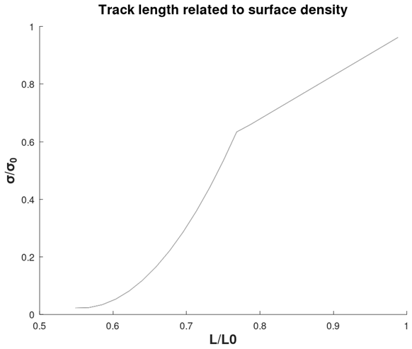
Figure B1 Reduced surface track density ${\frac{\mathit{\sigma }}{\mathit{\sigma }}}_{\mathrm{0}}^i$ as a function of the reduced c-axis projected track length $\frac{l^i}{L_{\mathrm{0}}}$. The track lengths are c-axis projected. The relations Eq. (B2) and (B3) are approximations to the relation given by Raymond Donelick (personal communication, 2026).

Appendix C

The vectors and the matrix G are shown below to help the reader keeping track of their mutual alignments. 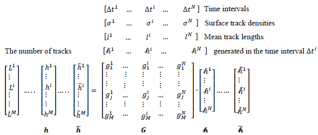Lⁱ is the track length binning, h the observed histogram (Data), $\stackrel{\mathrm{̃}}{\mathit{h}}$ the forward calculated approximation to data, G the matrix of laboratory annealed tracks, 𝔥 with elements 𝔥ⁱ being the histogram of tracks generated in the time interval Δtⁱ, $\stackrel{\mathrm{̃}}{\mathfrak{h}}$ the deconvolved track length histogram with elements ${\stackrel{\mathrm{̃}}{\mathfrak{h}}}^i$ of tracks generated in the time interval Δtⁱ.

Appendix D

In this appendix the variance-covariance matrixes for data C_H and prior C_P are presented. C_H is defined as given in Jensen and Hansen (2021). The number of track length measurements are usually restricted to a prior fixed number e.g., one hundred. The expected variance of the number of counted tracks in each histogram column is therefore calculated as being multinomial. They are the diagonal values of the variance-covariance matrix:

$$\begin{array}{}\text{(D1)}& {\mathbf{C}}_{\mathrm{H}}\left(j,j\right)=D{P}_{\mathrm{H}}^j(\mathrm{1}-P_{\mathrm{H}}^j)\mathrm{for}j=\mathrm{1}\mathrm{\dots }M,\end{array}$$

where M is the number of bins, $P_{\mathrm{H}}^j=d_{\mathrm{obs}}^j/D$ is the probability of the observed data $d_{\mathrm{obs}}^j$. D is the number of measured tracks. The covariances are off diagonal:

$$\begin{array}{}\text{(D2)}& {\mathbf{C}}_{\mathrm{H}}\left(l,j\right)=-D{P}_{\mathrm{H}}^l{P}_{\mathrm{H}}^j\mathrm{for}l\ne j.\end{array}$$

Prior values and variances are defined so that positive posterior values (positive histogram columns) are promoted and so that restrictions on the shape of the posterior histogram are not too hard. For example, in an extreme case, it is allowed that all tracks end up in a single column. This is an improvement to the definitions given in Jensen and Hansen (2021). The probability of the default priors is $P_{\mathrm{p}}^j=\frac{h_{\mathrm{prior}}^j}{D}=\frac{D/N}{D}=\mathrm{1}/N$ since the priors are equally distributed over the bins. The diagonal values of the covariance-variance matrix are then

$$\begin{array}{}\text{(D3)}& {\mathbf{C}}_{\mathrm{p}}\left(j,j\right)=qD{P}_{\mathrm{p}}^j\left(\mathrm{1}-P_{\mathrm{p}}^j\right)=D^{\mathrm{2}}\mathrm{for}j=\mathrm{1}\mathrm{\dots }N,\end{array}$$

where the default factor $q=\frac{D}{N(\mathrm{1}-\frac{\mathrm{1}}{N})}$ is chosen to ensure room for the possibility that all posterior tracks end up in a single bin. N is the number of prior bins. The covariances are off diagonal:

$$\begin{array}{}\text{(D4)}& {\mathbf{C}}_{\mathrm{H}}\left(l,j\right)=-f^{p}D{P}_{\mathrm{p}}^l{P}_p^j\mathrm{for}l\ne j.\end{array}$$