CoRSEER: the calculator of rock surface exposure age and erosion rates for luminescence rock surface exposure dating

Luminescence rock surface exposure dating (LRSED) estimates the duration of rock surface exposure and the rate of erosion by analysing changes in luminescence with depth below the surface. The wider use of this method has been slowed by limitations in mathematical analysis, such as the subjective selection of the deep plateau for profile normalisation, inconsistent modelling choices across studies, and the lack of a unified inverse-modelling workflow that delivers both parameter estimates and uncertainty bounds. We introduce the Calculator of Rock Surface Exposure Age and Erosion Rates (CoRSEER), an open-source MATLAB application that standardises the full workflow from luminescence depth profiles to exposure and erosion history. CoRSEER first normalises profiles objectively using weighted three-parameter logistic sigmoidal fitting to identify the saturation level and profile shape. It then simulates profile evolution with a finite-difference forward model that includes ambient-radiation-induced signal growth, depth-dependent bleaching described by a surface bleaching rate, attenuation coefficient, and advection caused by erosion. Finally, CoRSEER performs Monte Carlo inversion to estimate calibration parameters from known-age calibration samples, apparent exposure ages for unknown samples, and steady or stepwise erosion histories while reporting the best-fit and uncertainty ranges from likelihood-based filtering. We tested all three modules by reanalysing published datasets from multiple regions, including 23 calibration samples from the original dataset. For a representative calibration profile, CoRSEER-I improved the fit (coefficient of determination of 0.928 compared with 0.868 for the literature dataset) and substantially tightened the uncertainty bounds after objective renormalisation. Across the compiled studies, the CoRSEER-derived apparent ages cluster close to the one-to-one line relative to the published values and span approximately 1 year to 8.5 thousand years, while erosion estimates for a benchmark case remain comparable to the literature results. These results show that objective normalisation plus a transparent, standardised inversion framework can materially improve the reproducibility of luminescence rock surface exposure dating and support consistent inter-study comparisons of exposure and erosion history.

1 Introduction

Reconstructing the timing of rock surface exposure and erosion history is crucial in geomorphology because it links climate, tectonics, and surface processes that shape the landforms observed today (Molnar and England, 1990). Generally, there are two major reconstruction scenarios: (i) Establishing the exposure ages of host rocks (e.g., valley walls, bedrock, or strath surface) that can predict the age of the natural (e.g., deglaciation) and anthropogenic (e.g., stripping of regolith and quarrying) events that create a freshly exposed surface (Owen and Dortch, 2014; Gliganic et al., 2019). (ii) The transportation, deposition, and reworking histories of transportable clasts, such as cobbles and boulders (Luo et al., 2018). Furthermore, establishing the erosion rates of these rock surfaces provides information on the interactions between climate and landforms (Burbank et al., 1996). Evaluating the exposure-erosion history provides chronological and quantitative constraints on landscape evolution (Colman, 1981).

Terrestrial cosmogenic nuclide (TCN) dating has been extensively used to quantify rock surface exposure age and erosion rate (Lal, 1991; Balco et al., 2008; Dunai, 2010; Schaefer et al., 2022). ¹⁰Be dating, the most commonly used technique, is sensitive only above the millennial timescale (Schaefer et al., 2022). Furthermore, the unique concentration of ¹⁰Be can provide infinitely many pairs of exposure–erosion histories (Lehmann et al., 2019a) when the growth of ¹⁰Be is in a transient state; lower exposure-lower erosion may have a similar effect to higher exposure–higher erosion. Thus, an independent chronometer and/or the use of an additional nuclide is required to constrain both the exposure and erosion histories. Furthermore, the choice of different scaling models has a high impact on the derived exposure ages, and because of the unavailability of a production rate calibration site in most geologically significant sites (e.g., the Himalayan-Tibetan orogen), this problem becomes more critical (Owen and Dortch, 2014).

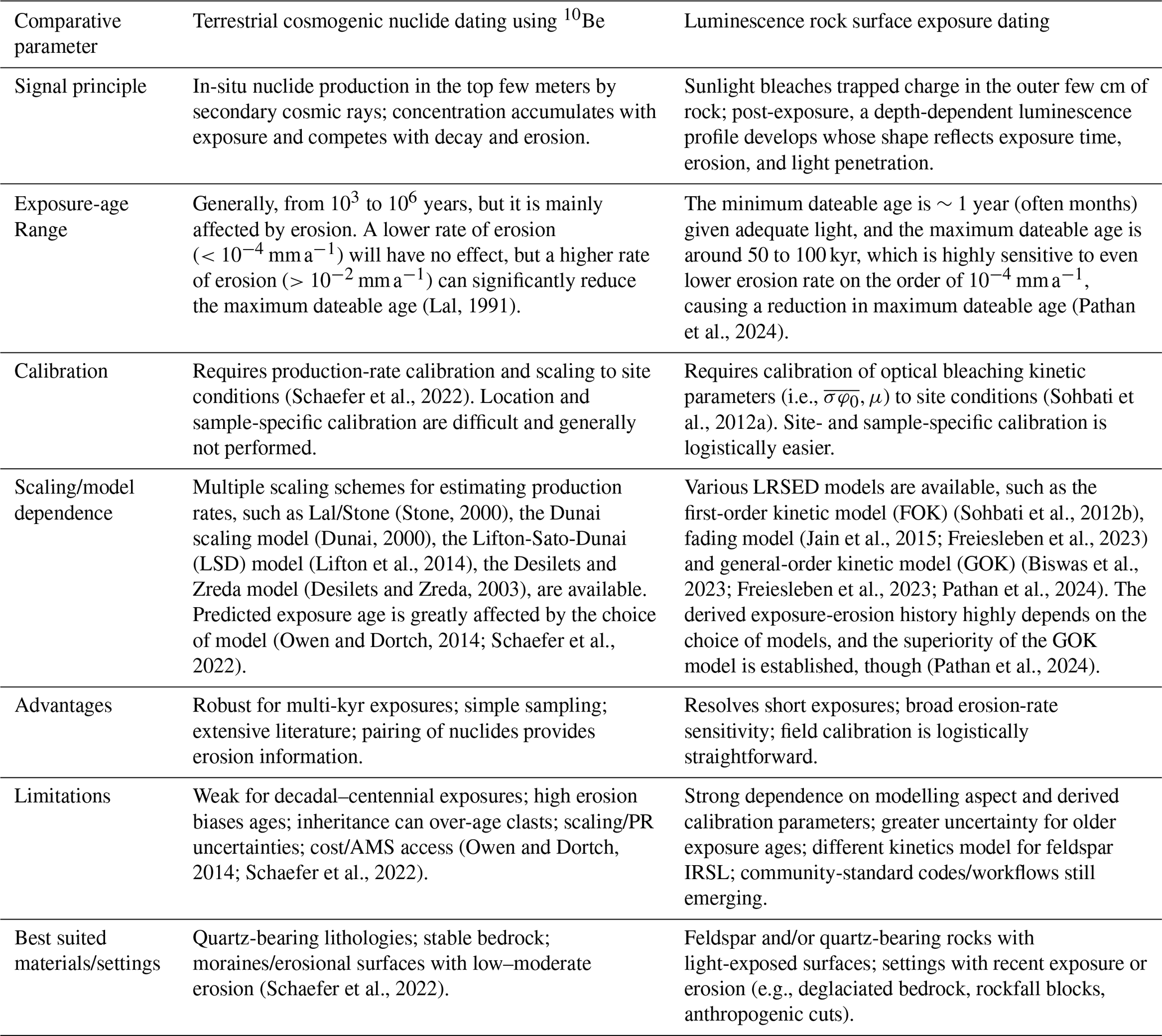
The introduction of the novel luminescence rock surface exposure dating (LRSED) has shown promising possibilities for overcoming some of these limitations and providing an additional independent chronometer. When rock is shielded from sunlight (part of the host rock or covered by opaque materials) and exposed to ambient radiation over Myr timescales, the ionising radiation fills electron traps to field saturation in minerals such as quartz and feldspar (Wintle and Murray, 2006). When exposed to sunlight, it penetrates the rock surface, causing instantaneous detrapping of electrons, that is, bleaching of the luminescence signal on the surface. As the photon flux attenuates with depth, the bleaching rate decreases, causing a sigmoidal distribution of luminescence signals, also called the luminescence depth profile (LDP) (Sohbati et al., 2011, 2012a). The LDP is highly sensitive to exposure and erosion but weakly sensitive to ambient dose rates. The exposure causes deeper propagation of the LDP, erosion cause advection towards the surface and ambient-dose-driven signal growth modifies its shape and position (Sohbati et al., 2018; Lehmann et al., 2019a). Even exposure of <1 year can be significant enough to cause a sigmoidal distribution. Conversely, erosion at extremely low erosion rates (order of 10⁻⁵ mm a⁻¹) can cause measurable advection of the LDP (Pathan et al., 2024). We argue that LRSED has the potential to act as a complementary method to TCN dating, and the LRSED-TCN coupled framework has been introduced in a few studies (Sohbati et al., 2018; Lehmann et al., 2019a; Smedley et al., 2021; Sohbati and Hippe, 2023). A comparison of TCN and LRSED dating is shown in Table 1.

Table 1 A comparison of TCN and LRSED.

2 Model

The choice of the incorporated model significantly affects the chronology derived using the LRSED. Thus, it is crucial to include the most accurate, peer-reviewed, simple, and flexible model that can encompass all the geological scenarios for the most robust chronology. This section reviews the LRSED models and discusses the model adopted in this study.

2.1 Laskaris and Liritzis (2011)

This is the first parametric fit function presented for luminescence rock surface exposure dating (Laskaris and Liritzis, 2011). This was suggested for both OSL and TL.

$$\begin{array}{}\text{(1)}& L(x;a_{\mathrm{1}},b_{\mathrm{1}},c_{\mathrm{1}},d_{\mathrm{1}})=a_{\mathrm{1}}+{\displaystyle \frac{b_{\mathrm{1}}}{\mathrm{2}}}\text{erfc}\left({\displaystyle \frac{\ln \left(\frac{x}{c_{\mathrm{1}}}\right)}{d_{\mathrm{1}}\sqrt{\mathrm{2}}}}\right)\end{array}$$

where L is the distribution of luminescence signal with respect to depth, and it depends on the fitting parameters as a₁, b₁, c₁, and d₁. While this empirical model enables precise fitting to the luminescence depth profile, it does not explain the luminescence mechanism inside the rock, and the derived fitting parameters are not linked to the natural kinetic parameters. Additionally, this model assumes zero erosion conditions, which are not always achievable. Thus, this model was not incorporated into any further LRSED studies.

2.2 Sohbati et al. (2018)

Sohbati et al. (2018) proposed a model whereby the instantaneous concentration of trapped electrons n at depth x is:

$$\begin{array}{}\text{(2)}& {\displaystyle \frac{\mathrm{d}n}{\mathrm{d}t}}=(N-n)F\left(x\right)-nE\left(x\right)\end{array}$$

where,

$$\begin{array}{}\text{(3)}& {\displaystyle }E\left(x\right)=\stackrel{\mathrm{‾}}{\mathit{\sigma }{\mathit{\phi }}_{\mathrm{0}}}{e}^{-\mathit{\mu }x}\text{(4)}& {\displaystyle }F=\dot{D}\left(x\right)/D_{\mathrm{0}}\end{array}$$

With the boundary conditions n=N at t=0, the analytical solution was evaluated as

$$\begin{array}{}\text{(5)}& {\displaystyle \frac{n(x,t)}{N}}={\displaystyle \frac{E\left(x\right)e^{-t\left[E\right(x)+F]}+F}{E\left(x\right)+F}}\text{(6)}& {\displaystyle \frac{n(x,t)}{N}}={\displaystyle \frac{\stackrel{\mathrm{‾}}{\mathit{\sigma }{\mathit{\phi }}_{\mathrm{0}}}{e}^{-\mathit{\mu }x}{e}^{-t(\stackrel{\mathrm{‾}}{\mathit{\sigma }{\mathit{\phi }}_{\mathrm{0}}}{e}^{-\mathit{\mu }x}+\frac{\dot{D}}{D_{\mathrm{0}}})}+\frac{\dot{D}}{D_{\mathrm{0}}}}{\stackrel{\mathrm{‾}}{\mathit{\sigma }{\mathit{\phi }}_{\mathrm{0}}}{e}^{-\mathit{\mu }x}+\frac{\dot{D}}{D_{\mathrm{0}}}}}\end{array}$$

The model was further improved by incorporating an erosion scenario (Sohbati et al., 2018).

$$\begin{array}{}\text{(7)}& {\displaystyle }x\left(t\right)=x_{\mathrm{0}}-\dot{\mathit{\epsilon }}t\text{(8)}& {\displaystyle }\begin{array}{rl}{\displaystyle }E\left(x\right(t\left)\right)& {\displaystyle }=\stackrel{\mathrm{‾}}{\mathit{\sigma }{\mathit{\phi }}_{\mathrm{0}}}{e}^{-\mathit{\mu }(x_{\mathrm{0}}-\dot{\mathit{\epsilon }}t)}=\left(\stackrel{\mathrm{‾}}{\mathit{\sigma }{\mathit{\phi }}_{\mathrm{0}}}{e}^{-\mathit{\mu }{x}_{\mathrm{0}}}\right)e^{\mathit{\mu }\dot{\mathit{\epsilon }}t}\\ {\displaystyle }& {\displaystyle }=E_{\mathrm{0}}{e}^{\mathit{\mu }\dot{\mathit{\epsilon }}t}\end{array}\text{(9)}& {\displaystyle \frac{\mathrm{d}n}{\mathrm{d}t}}=(N-n)F-n{E}_{\mathrm{0}}{e}^{\mathit{\mu }\dot{\mathit{\epsilon }}t}\end{array}$$

where the analytical solution, expressed as a confluent hypergeometric function M, is:

$$\begin{array}{}\text{(10)}& {\displaystyle \frac{n(x,\dot{\mathit{\epsilon }})}{N}}=M\left(\mathrm{1},\mathrm{1}+{\displaystyle \frac{F}{\mathit{\mu }\dot{\mathit{\epsilon }}}},-{\displaystyle \frac{E\left(x\right)}{\mathit{\mu }\dot{\mathit{\epsilon }}}}\right)\end{array}$$

The analytical solution improves the feasibility of modelling by incorporating the effects of dose rates, first-order kinetics (FOK) decay behaviour and erosion. However, in the case of polymineral or feldspar samples, where the infrared stimulated luminescence (IRSL) of feldspar minerals exhibits non-first-order decay, the general-order kinetic (GOK) model is more suitable for these samples.

2.3 Freiesleben et al. (2023) model

Freiesleben et al. (2023) developed this model to incorporate GOK:

$$\begin{array}{}\text{(11)}& {\displaystyle \frac{\mathrm{d}n}{\mathrm{d}t}}=-E_{\dot{\mathit{\epsilon }}}(x,t)n^r\end{array}$$

where r is the order of kinetics.

$$\begin{array}{}\text{(12)}& {\displaystyle }{E}_{\dot{\mathit{\epsilon }}}(x,t)=\stackrel{\mathrm{‾}}{\mathit{\sigma }{\mathit{\phi }}_{\mathrm{0}}}{e}^{-\mathit{\mu }(x_{\mathrm{0}}-\dot{\mathit{\epsilon }}t)}\text{(13)}& {\displaystyle }n(x,t_{\dot{\mathit{\epsilon }}})=\left[\right(r-\mathrm{1}\left)t_{\dot{\mathit{\epsilon }}}E\right(x)+n^{\mathrm{1}-r}{]}^{\frac{\mathrm{1}}{\mathrm{1}-r}}\end{array}$$

where the apparent exposure time is given as

$$\begin{array}{}\text{(14)}& t_{\mathit{\epsilon }}={\displaystyle \frac{\mathrm{1}}{\mathit{\mu }\dot{\mathit{\epsilon }}}}(\mathrm{1}-e^{-\mathit{\mu }\dot{\mathit{\epsilon }}t})\end{array}$$

This model considers the order of kinetics and erosion scenario but ignores the effect of the dose rate on LDP propagation. However, in natural environments, the dose rate considerably affects the propagation of LDP over a longer timescale (>10³ years), and this effect is amplified with an increase in the order of kinetics (Pathan et al., 2024). This model also assumes a constant average rate of erosion, which may not be applicable in different erosion scenarios, such as step-function or stochastic histories (Ganti et al., 2016; Brown and Moon, 2019; Lehmann et al., 2019a).

2.4 Model framework after Lehmann et al. (2019a), Biswas et al. (2023) and Pathan et al. (2024)

The modelling framework adopted in this study brings together the current understanding of rock-surface luminescence signal evolution within a single computational framework. It includes: (1) general-order kinetics, (2) advection through the natural mechanism of erosion, and (3) ambient dose-rate-driven signal accumulation. This formulation was required to simulate the luminescence-depth profile more accurately and builds upon earlier work by Lehmann et al. (2019a), Biswas et al. (2023), and Pathan et al. (2024). Lehmann et al. (2019a) introduced the advection term in response to erosion as $\dot{\mathit{\epsilon }}\frac{\mathrm{d}\stackrel{\mathrm{‾}}{n}}{\mathrm{d}x}$ but for the FOK (r=1) in addition to earlier models. Thus, the instantaneous change in normalised luminescence $\stackrel{\mathrm{‾}}{n}$ (see Sect. 3.1 for normalisation procedure) with respect to time t at depth x, is expressed as:

$$\begin{array}{}\text{(15)}& \begin{array}{rl}{\displaystyle \frac{\mathrm{d}\stackrel{\mathrm{‾}}{n}}{\mathrm{d}t}}& {\displaystyle }={\left\{{\displaystyle \frac{\dot{D}}{D_{\mathrm{0}}}}(\mathrm{1}-\stackrel{\mathrm{‾}}{n})\right\}}_{\text{growth}}-\mathit{\{}{\stackrel{\mathrm{‾}}{n}}^r{\stackrel{\mathrm{‾}}{\mathit{\sigma }\mathit{\phi }}}_{\mathrm{0}}{e}^{-\mathit{\mu }x}{\mathit{\}}}_{\text{decay}}\\ {\displaystyle }& {\displaystyle }+{\left\{\dot{\mathit{\epsilon }}{\displaystyle \frac{\mathrm{d}\stackrel{\mathrm{‾}}{n}}{\mathrm{d}x}}\right\}}_{\text{erosion}}\end{array}\end{array}$$

This model can be solved using a finite-difference method with a second-order upwind scheme for the advection term rather than altering the depth term (Sohbati et al., 2018). Furthermore, Biswas et al. (2023) modified this model for a zero erosion scenario by incorporating GOK (r>1) in the decay term and demonstrated the severe underestimation of the exposure age if FOK was used. Pathan et al. (2024) solved the GOK model (Eq. 15) for a non-zero erosion scenario and reported an overestimation of the erosion rate when FOK was used. Thus, we incorporate the most recent model, as in Eq. (15), into the mathematical framework of CoRSEER.

The model accounts for signal growth due to environmental dose rate, depth-dependent light attenuation, nonlinear bleaching behaviour of IRSL signals, and advective loss of material due to surface erosion. Therefore, it provides a physically consistent framework for simulating LDP evolution under both exposure and erosion. This class of model has been used in several studies. Lehmann et al. (2019a) and Elkadi et al. (2022) used this model assuming FOK (r=1) to jointly invert ¹⁰Be cosmogenic nuclide data and LRSED profiles, allowing erosion histories and erosion-corrected exposure ages to be constrained through complementary dating systems. Smedley et al. (2021), Brill et al. (2021), and other studies also applied this framework for reconstructing erosion histories, generally assuming FOK.

The incorporation of general-order kinetics is particularly important for feldspar-based IRSL signals, where slower and non-exponential bleaching behaviour is commonly observed. The FOK model assumes simple exponential decay with (r=1), whereas the GOK model introduces a kinetic-shape parameter (r), which can represent slower bleaching behaviour observed in feldspar signals (Duller, 1997; Chen and Leung, 2003; Guralnik et al., 2015). Previous studies have shown that the use of FOK may lead to underestimation of exposure ages and overestimation of erosion rates, in some cases by up to an order of magnitude (Biswas et al., 2023; Pathan et al., 2024; Luo et al., 2026). By embedding this model within CoRSEER, we provide a reproducible platform for forward and inverse modelling of LRSED profiles, enabling more consistent reconstruction of exposure–erosion histories. The prerequisites for CoRSEER, sampling strategy, and sample-processing methods for LRSED are provided in Sects. S1–S3 in the Supplement, respectively.

3 Methodology

CoRSEER is a MATLAB-based app designed to streamline the quantification of rock surface exposure age (for uneroded surfaces) and erosion histories (for eroded surfaces) through inverse modelling of luminescence depth profiles. The workflows are as follows.

3.1 Normalisation of experimental data

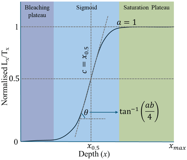
To eliminate the effect of intersample variability (mass and luminescence production efficiency), the test-dose normalised luminescence ($L_x/T_x$) was measured at different depths to generate the LDP. The LDP is further adjusted (or normalised) to plateau at 1 to facilitate further mathematical operations (Sohbati et al., 2012a). Traditionally, users select a depth beyond which the experimental LDP is assumed to be saturated through visual inspection and compute the mean $L_x/T_x$ of all points thereafter to normalise the entire profile. However, the high scatter in the saturation region often leads to subjective depth selection, introducing human error and bias. The incorrectly identified plateau can systematically distort the normalised signals and skew the kinetic parameter estimation. To overcome this, we present an empirical normalisation using the sigmoidal curve fitting (SCF) method. We chose the following three-parameter logistic sigmoidal function (Kaufmann, 1981) to model the luminescence-depth profile:

$$\begin{array}{}\text{(16)}& f\left(x\right)={\displaystyle \frac{a}{\mathrm{1}+\exp [-b(x-c\left)\right]}}\end{array}$$

Here, a is the upper asymptote, the maximum value the function can attain as x∼∞, denotes the saturation luminescence intensity (or $L_x/T_x$), and b is the growth rate, which controls the steepness of the curve. A higher b indicates a steeper transition of $L_x/T_x$ with depth. c represents the inflection point or x_0.5, that is, the depth at which half of the saturation signal is reached (Fig. 1). To derive a, b, and c, we fitted Eq. (16) to the experimental LDP using weighted nonlinear least-squares regression in MATLAB. The initial guesses for fitting parameters were set to $a_{\mathrm{0}}=max\left(\frac{L_x}{T_x}\right)$, b₀=1 and c₀=median(x). We enforced bounds to ensure physically meaningful solutions: (a) lower bounds: $[\mathrm{0},\mathrm{0},\mathrm{0}]$, (b) upper bounds: $[\mathrm{\infty },\mathrm{\infty },max(x\left)\right]$, and provided the weight factors (w_i) as $w_i=\frac{\mathrm{1}}{\mathit{\alpha }}$ where α is the fractional error. The experimentally observed LDP ($L_x/T_x$ vs. depth) was normalised with the respective a value for each sample and referred as SCF-normalised LDP. This approach was used to identify the plateau and normalise the experimental data. This method removes bias, improves reproducibility, and ensures a consistent LDP normalisation algorithm across diverse datasets by eliminating manual intervention.

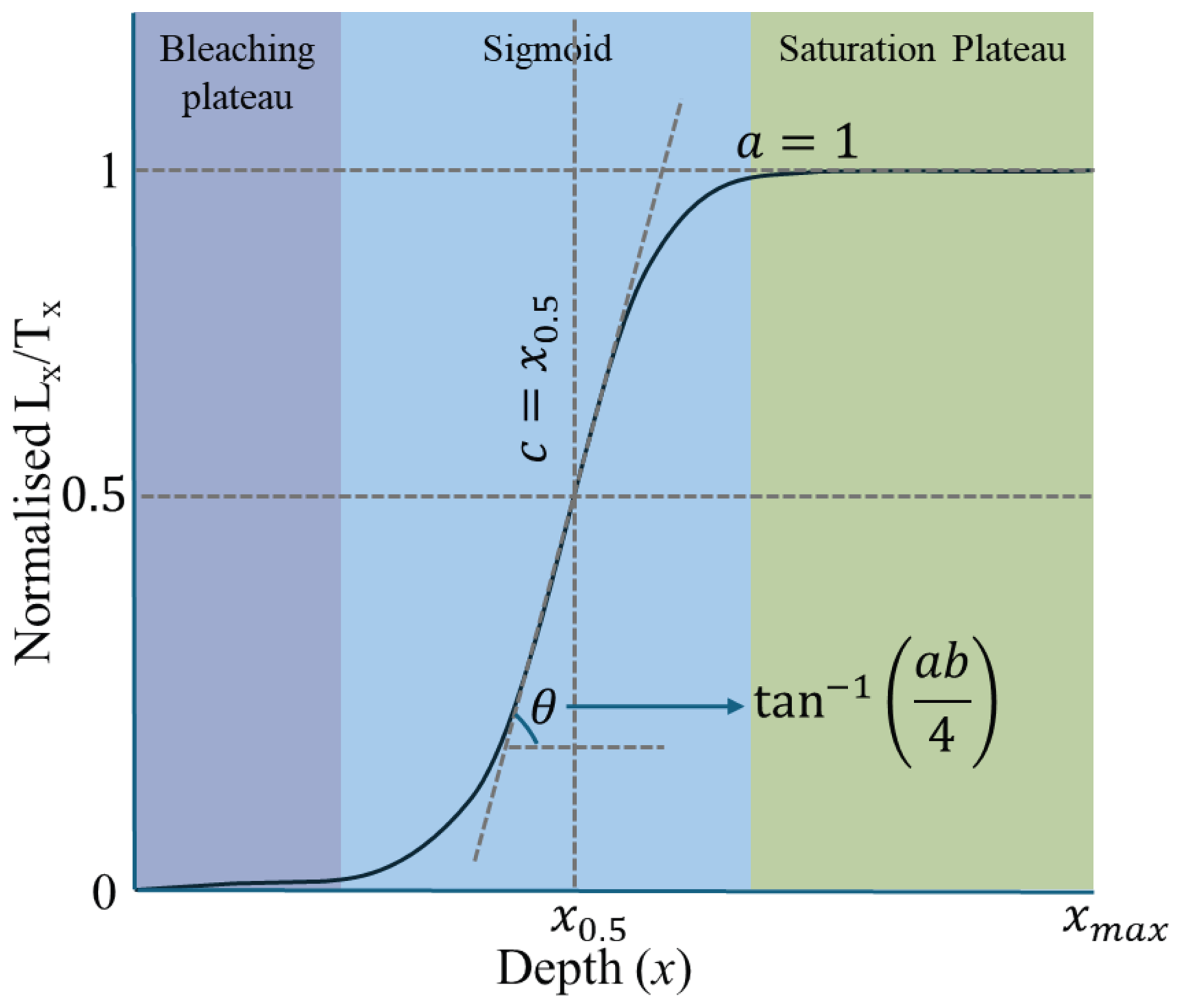
Figure 1 The luminescence-depth profile (LDP) sigmoidal shape consists of three distinct regions: (i) the near-surface bleaching plateau, (ii) the middle slope ($\tan \mathit{\theta }=\left(\frac{ab}{\mathrm{4}}\right)$ at c=x_0.5) of sigmoidal shape, and (iii) the deep saturation plateau of magnitude “a”.

3.2 Inverse modelling in CoRSEER

In inverse modelling, multiple LDPs are simulated by solving Eq. (15) using the finite difference method for two main scenarios: (a) varying kinetic parameters, $\stackrel{\mathrm{‾}}{\mathit{\sigma }{\mathit{\phi }}_{\mathrm{0}}}$, and μ (keeping the exposure-erosion history as fixed) or (b) by varying the exposure-erosion history (keeping $\stackrel{\mathrm{‾}}{\mathit{\sigma }{\mathit{\phi }}_{\mathrm{0}}}$, and μ as fixed). For a calibration sample (known exposure-erosion history), kinetic parameters ($\stackrel{\mathrm{‾}}{\mathit{\sigma }{\mathit{\phi }}_{\mathrm{0}}}$, and μ) are randomly varied, whereas for natural samples (known $\stackrel{\mathrm{‾}}{\mathit{\sigma }{\mathit{\phi }}_{\mathrm{0}}}$, and μ), the exposure-erosion history is randomly varied. The other kinetic parameters, $\dot{D}$, D₀, and r are constrained independently using DRAC (Durcan et al., 2015; Sohbati et al., 2018), IRSL dose-response curve (Wintle and Murray, 2006) and fitting decay of IRSL with light exposure (Biswas et al., 2023), respectively. These parameters are user-defined in CoRSEER. The most probable, or best-fitting, LDPs and corresponding parameters are constrained by comparing the simulated LDPs (${\stackrel{\mathrm{‾}}{n}}_{\text{sim}}$) and experimentally observed SCF normalised LDP (${\stackrel{\mathrm{‾}}{n}}_{\text{obs}}$) and by minimising the chi-square misfit (χ²) and maximising the likelihood, following the approach by Lehmann et al. (2019a).

$$\begin{array}{}\text{(17)}& {\displaystyle }{\mathit{\chi }}^{\mathrm{2}}=\sum _{i=\mathrm{1}}^l{\displaystyle \frac{{\left((\stackrel{\mathrm{‾}}{n}{)}_{\text{obs}}^{\left(i\right)}-(\stackrel{\mathrm{‾}}{n}{)}_{\text{sim}}^{\left(i\right)}\right)}^{\mathrm{2}}}{{\mathit{\delta }}^{\mathrm{2}}}}\text{(18)}& {\displaystyle }\text{likelihood}=P=e^{-{\mathit{\chi }}^{\mathrm{2}}/\mathrm{2}}\text{(19)}& {\displaystyle }{P}_{\text{norm}}^k={\displaystyle \frac{P_k}{P_{\text{max}}}}\end{array}$$

where l is the number of experimental data points, δ is the standard deviation of the residual between the observed experimental profile and the best-fitting sigmoidal curve, divided by “a” factor, P_k is the likelihood value associated with the simulated LDP numbered as k, P_max is maximum-likelihood, which is associated with the best-fitting synthetic LDP and $P_{\text{norm}}^k$ is the normalised likelihood value associated with the simulated LDP numbered as k. The best LDP and corresponding parameters were selected by applying the Monte Carlo acceptance criterion as $P_{\text{norm}}^k>U$, where U is a random number between zero and one. Finally, CoRSEER establishes the values of best-fit, median, ±1δ, and ±2δ for all required parameters with confidence intervals.

3.2.1 Calibration

CoRSEER-I module constrains $\stackrel{\mathrm{‾}}{\mathit{\sigma }{\mathit{\phi }}_{\mathrm{0}}}$ and μ from the SCF normalised LDP of calibration sample (known exposure age and known erosion rate). The inverse modelling (described above) is performed with fixed input parameters $\dot{D}$, D₀, r, t, and $\dot{\mathit{\epsilon }}$ and random selection of $\stackrel{\mathrm{‾}}{\mathit{\sigma }{\mathit{\phi }}_{\mathrm{0}}}$ and μ from a user-defined range for a large number of iterations. It must be mentioned that erosion is assumed to be negligible for the young calibration sample. However, for the older calibration sample, erosion might not be zero, which may bias the parameter estimates. CoRSEER-I has the option to include erosion rate ($\dot{\mathit{\epsilon }}>\mathrm{0}$), if known.

The parameter pair ($\stackrel{\mathrm{‾}}{\mathit{\sigma }{\mathit{\phi }}_{\mathrm{0}}}$ and μ) associated with the lowest normalised chi-square is designated the best-fit bleaching parameter. To assess uncertainty, CoRSEER-I filters the entire chi-square field using a probabilistic threshold: all solutions where $P_{\text{norm}}^k>\text{rand}(m,m)$ (following the method of Pathan et al., 2024) are retained, and their median and ±δ uncertainty bounds are reported. This approach ensures the statistical robustness and physical interpretability of the calibrated parameters. The details of the input, mechanism, and output of CoRSEER-I are discussed in Sect. S4.1 in the Supplement. These location- and rock-type-specific calibration parameters ($\stackrel{\mathrm{‾}}{\mathit{\sigma }{\mathit{\phi }}_{\mathrm{0}}}$ and μ) are used as inputs in exposure age and erosion rate calculation.

A representative analysis was performed on the LDP of the available literature data ROAD02 (Smedley et al., 2021). As we are solving for only one LDP corresponding to the IRSL50 signal, the LDP is termed IR50_ROAD02. The LDP was normalised to 1 by dividing the mean deep-plateau $L_x/T_x$. This road-cut sample has an exposure age of 57 a (when the LDP was generated). The other parameters are r=1, $\dot{D}=\mathrm{4.76}$ ± 0.15 Gy kyr⁻¹, and D₀=500 Gy. The inverse modelling is performed for 500×500 pairs of $\stackrel{\mathrm{‾}}{\mathit{\sigma }{\mathit{\phi }}_{\mathrm{0}}}$ (ranging from 10⁻¹⁰ to 10⁰ s⁻¹, spacing in log-scale) and μ (ranging from 0 to 4 mm⁻¹), and considering no erosion. After the calibration is completed, CoRSEER generates three diagnostic plots, as shown in Fig. 2a–c.

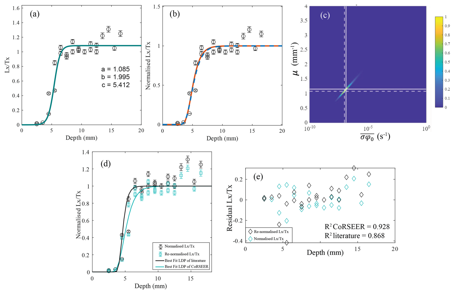
Figure 2 Reevaluation of the IR50 calibration parameters for sample ROAD02 (IR50_ROAD02) (Smedley et al., 2021). (a) The natural IR50 $L_x/T_x$ depth profiles (hollow circles) and associated sigmoidal fit (teal solid line). Although the normalisation was already performed by Smedley et al. (2021), the fitted amplitude showed a=1.085, indicating ∼8.5 % under-normalisation. Parameters b and c indicate the steepness and x_0.5, respectively. (b) The simulated LDPs for best-fit (dashed blue) and median (solid orange) calibration parameters associated with the SCF-normalised LDP (hollow circles). The precise overlap between both simulated LDPs shows a strong agreement between the best-fit and median values, indicating plausible fitting strategies. (c) Probability likelihood distribution in $\stackrel{\mathrm{‾}}{\mathit{\sigma }{\mathit{\phi }}_{\mathrm{0}}}$ and μ space from Bayesian inversion. The dashed lines represent the best-fitting values, and the solid line represents the median of the filtered values using the criteria described in Sect. 3.2.1. (d) Direct comparison of the literature-normalised profile (black circles) and SCF-normalised profile (cyan squares) using CoRSEER-I alongside their corresponding best-fit simulated luminescence depth profile (black and cyan lines). Both datasets show comparable x_0.5, but there is a slight change in the slope after renormalisation. (e) Residuals (data−model) as a function of depth for both fits, highlighting the improved agreement for CoRSEER-I. The coefficient of determination increases from R²=0.868 (literature handling) to R²=0.928 (CoRSEER-I), indicating a tighter, more precise fit to the same underlying measurements.

The normalisation factor in the SCF analysis was estimated as a=1.085 (Fig. 2a), which shows the presence of under-normalisation, and the profiles were further renormalised (SCF normalisation) using this factor for accuracy. Figure 2b and c show the plausible fitting using CoRSEER-I comparable to the fitting seen in the literature (Fig. 6g of Smedley et al., 2021). The resulting best-fitting $\stackrel{\mathrm{‾}}{\mathit{\sigma }{\mathit{\phi }}_{\mathrm{0}}}$ and μ values are $\mathrm{1}\times {\mathrm{10}}^{-\mathrm{7}}$ s⁻¹ and 1.08 mm⁻¹ which vary significantly from reported values of $\mathrm{6.67}\times {\mathrm{10}}^{-\mathrm{6}}$ s⁻¹ (overestimated approximately by an order of 2) and 2.1 mm⁻¹ (overestimated by factor of ∼2) by Smedley et al. (2021). Furthermore, the ±1δ range for $\stackrel{\mathrm{‾}}{\mathit{\sigma }{\mathit{\phi }}_{\mathrm{0}}}$ is reduced from $\mathrm{3.50}\times {\mathrm{10}}^{-\mathrm{7}}$–$\mathrm{1.27}\times {\mathrm{10}}^{-\mathrm{4}}$ s⁻¹ to $\mathrm{6.39}\times {\mathrm{10}}^{-\mathrm{8}}$–$\mathrm{3.11}\times {\mathrm{10}}^{-\mathrm{7}}$ s⁻¹, and μ is reduced from 1.4–2.6 to 1.00 to 1.31 mm⁻¹, showing the narrowing of the uncertainty interval. We investigated the reason for this discrepancy between the results by comparing the manually normalised LDP (literature) from the SCF-normalised LDP (factor a=1.085). We plotted the simulated profiles using the calibration dataset associated with both LDPs (literature and CoRSEER-I, respectively). Figure 2d shows that there is no tangible depth difference between the literature and CoRSEER-I generated profiles, but we see a noticeable difference in the slope of the LDPs. The estimated R² values were 0.868 for the literature dataset and 0.928 for CoRSEER-I, indicating greater precision in fitting with CoRSEER, as shown in Fig. 2e.

Despite the slight difference in the R² values, the evaluated kinetic parameters varied significantly. The apparent reason for this discrepancy likely results from (1) SCF normalisation of the LDP and (2) the Fitting Strategy.

3.2.2 Age estimation

This module evaluates the exposure age from the LDP of an unknown sample for a no-erosion scenario. If the sample had an erosion history, the derived age would be the apparent exposure age (t_app). The inverse modelling is performed with fixed input parameters, $\dot{D}$, D₀, r, $\stackrel{\mathrm{‾}}{\mathit{\sigma }{\mathit{\phi }}_{\mathrm{0}}}$, μ and $\dot{\mathit{\epsilon }}$ and random selection of t from a user-defined range for a large number of iterations. A probabilistic threshold filter is applied (e.g., $P_{\text{norm}}^k>\text{rand}(m,\mathrm{1})$) to extract accepted LDPs from which the best-fitting age, median age and ±1δ age uncertainty are derived. The algorithm also calculates t_max, the maximum possible exposure age, which is associated with depth beyond which the LDP does not hold any information about exposure history (x_0.5,max). Here, we define $x_{\mathrm{0.5},\text{max}}<x_{\mathrm{0.5},\text{ss}}-\mathrm{1}/\mathit{\mu }$, as described by Sohbati et al. (2018). We simulated the evolution of x_0.5, the depth at which the luminescence signal reaches 50 % of the saturation signal. The simulation continued until x_0.5 asymptotically approached a steady-state depth of x_0.5,ss. The input, mechanism, and output of CoRSEER-II are discussed in Sect. S4.2 in the Supplement.

Here, we evaluated the exposure age of the rock avalanche boulder BALL02 (Smedley et al., 2021) (hereafter IR50_BALL02) using CoRSEER-II. The boulder was deposited and exposed due to the rock avalanche event dated to t_i=4.52 ± 0.27 ka. Smedley et al. (2021) estimated the erosion-uncorrected exposure age (t_app) as 8 ± 2 a, which was evaluated using $\dot{D}=\mathrm{3.32}$ ± 0.12 Gy kyr⁻¹, D₀=500 Gy, $\stackrel{\mathrm{‾}}{\mathit{\sigma }{\mathit{\phi }}_{\mathrm{0}}}=\mathrm{6.67}\times {\mathrm{10}}^{-\mathrm{6}}$ s⁻¹, μ=2.1 mm⁻¹, $\dot{\mathit{\epsilon }}=\mathrm{0}$ and r=1 (The calibration parameters were evaluated from ROAD02). Here, we replace the calibration parameters, $\stackrel{\mathrm{‾}}{\mathit{\sigma }{\mathit{\phi }}_{\mathrm{0}}}$, and μ with the values obtained in CoRSEER-I, $\stackrel{\mathrm{‾}}{\mathit{\sigma }{\mathit{\phi }}_{\mathrm{0}}}=\mathrm{1}\times {\mathrm{10}}^{-\mathrm{7}}$ s⁻¹, μ=1.08 mm⁻¹, and keeping the other parameters ($\dot{D}$, D₀, r) same. CoRSEER-II generates three diagnostic plots, as shown in Fig. 3a–c.

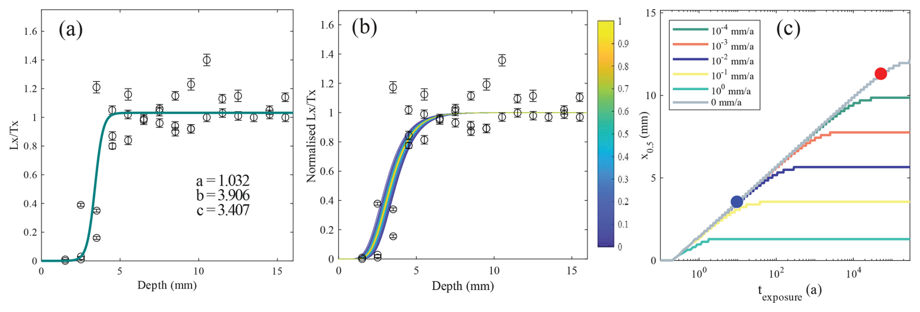
Figure 3 CoRSEER-II exposure-age inversion and erosion-diagnostic modelling for rock avalanche boulder IR50_BALL02. (a) Unknown natural IR50 $L_x/T_x$ depth profiles (hollow circles) and their sigmoidal fit (teal solid line). The fitted a=1.032 shows 3.2 % under normalisation, which was further used for SCF normalisation of the natural LDP. The b-value of 3.906 indicates a very steep slope. (b) The renormalised LDP (black hollow circles) and its corresponding Bayesian inversion fit resulting in the probability likelihood patch of ±δ exposure age LDP. Convergence towards the centre indicates an excellent fit to the model. (c) The evolution of x_0.5 for long-term exposure and constant erosion-rate (0, 10⁻⁴, 10⁻³, 10⁻², 10⁻¹, 10⁰, mm a⁻¹) scenarios using $\dot{D}=\mathrm{3.32}$ ± 0.12 Gy kyr⁻¹, D_o=500 Gy, ${\stackrel{\mathrm{‾}}{\mathit{\sigma }\mathit{\phi }}}_{\mathrm{0}}=\mathrm{1}\times {\mathrm{10}}^{-\mathrm{7}}$ s⁻¹, μ=1.08 mm⁻¹ and r=1. The blue-filled circle denotes the x_0.5,natural, taken as the c value of the current profile from panel (a). The red-filled marker plotted on the zero-erosion x_0.5 line indicates the no-erosion chronometer limit ($x_{\mathrm{0.5},\text{max}}<x_{\mathrm{0.5},\text{ss}}-\mathrm{1}/\mathit{\mu }$), showing that the profile could, in principle, record ages up to ∼52 ka if no ongoing erosion of the surface occurred.

The fitted value a=1.032 shows (Fig. 3a) the presence of mild inaccurate normalisation, and the unknown age LDP was renormalised. The impressive fitting of the SCF-normalised LDP with the accepted paths shows a successful inversion, as shown in Fig. 3b. The apparent exposure age calculated as ${\mathrm{9}}_{-\mathrm{1}}^{+\mathrm{2}}$ a using CoRSEER-II is comparable to 8 ± 2 a as derived by Smedley et al. (2021). Despite the significant difference in calibration parameters derived from CoRSEER-I and the literature, we observed almost the same ages. This can be explained by the fact that while performing a single calibration (Sohbati et al., 2012b), the ${\stackrel{\mathrm{‾}}{\mathit{\sigma }\mathit{\phi }}}_{\mathrm{o}}$ and μ can covary (Fig. 5c), and based on fitting strategies, both parameters can change. The calibration profile of higher $\log \left({\stackrel{\mathrm{‾}}{\mathit{\sigma }\mathit{\phi }}}_{\mathrm{o}}\right)$ and μ will overlap to lower $\log \left({\stackrel{\mathrm{‾}}{\mathit{\sigma }\mathit{\phi }}}_{\mathrm{o}}\right)$ and μ for the same age sample, but the magnitude of the slope of the sigmoid will be less for lower μ (Sohbati et al., 2018). Finally, this is affected by the precision of the model and fitting strategy used to account for the slope of the curvature.

Using the kinetic parameters given earlier, we simulate the propagation of the LDP by tracking the x_0.5 with a simulated exposure time (>10⁵ a) for different constant erosion rate scenarios ($\dot{\mathit{\epsilon }}={\mathrm{10}}^{-\mathrm{4}}$, 10⁻³, 10⁻², 10⁻¹, 10⁰, 0 mm a⁻¹), as shown in Fig. 3c. We plot two points on the no erosion x_0.5 line: (i) The x_0.5,natural (blue filled circle in Fig. 3c) corresponds to the apparent exposure age. (ii) x_0.5,max (red filled circle in Fig. 3c), depth of maximum exposure age ($x_{\mathrm{0.5},\text{max}}<x_{\mathrm{0.5},\text{ss}}-\mathrm{1}/\mathit{\mu }$). Thus, for a no-erosion scenario, the current sample can be dated up to an age of ∼52 ka, which is far higher than the actual exposure age (4.52 ± 0.27 ka) of the boulder. The highly underestimated apparent exposure age of 9 ± 1 a indicates that this sample underwent significant erosion. Assuming that the LDP is in a steady-state equilibrium, for current x_0.5,natural, the erosion rates may lie between 10⁻² and 10⁰ mm a⁻¹. This represents the plausible performance and application of CoRSEER-II to derive and diagnose the apparent exposure ages and provide insight into the possible erosion rate.

3.2.3 Erosion estimation

Here, we evaluated the erosion history of a rock surface undergoing step-function erosion. Although the natural erosion pattern is more stochastic, we prefer the step-function history for computational simplicity, as used in previous studies (Lehmann et al., 2019a, b; Smedley et al., 2021; Elkadi et al., 2022; Pathan et al., 2024). Using user-provided logarithmic spacing of exposure-erosion history, the CoRSEER-III creates two parameter arrays: erosion rates ($\dot{\mathit{\epsilon }}$) and exposure durations (t). If the erosion-corrected exposure age is known by any other independent method, the t can be replaced with its value. For each ($\dot{\mathit{\epsilon }},t$) pair, it simulates LDPs using a two-phase approach: Phase 1 with no erosion (from 0 to zero erosion exposure period (t_o)), and Phase 2 with constant erosion, $\dot{\mathit{\epsilon }}$ (for the period of t_s) ($t=t_{\mathrm{o}}+t_{\mathrm{s}}$, total exposure age). This forward modelling solves Eq. (15) using the finite difference method and produces the final simulated LDPs. We plot $\dot{\mathit{\epsilon }}$–t_s matrix and its associated $P_{\text{norm}}^k$ and interpret the exposure-erosion conditions. Furthermore, we perform a Gaussian distribution operation on $\dot{\mathit{\epsilon }}$ column associated with steady erosion onset exposure age (t_ss). The input, mechanism, and output of CoRSEER-III are discussed in Sect. S4.3 in the Supplement.

We evaluated the exposure-erosion history of IR50_BALL02, which was suspected to face significant erosion, as discussed in Sect. 3.2.2. Smedley et al. (2021) estimated the steady-state erosion rate (${\dot{\mathit{\epsilon }}}_{\text{ss}}$) and erosion onset exposure age (t_ss) as 0.066 mm a⁻¹ and 73 a, which was evaluated using $\dot{D}=\mathrm{3.32}$ ± 0.12 Gy kyr⁻¹, D₀=500 Gy, $\stackrel{\mathrm{‾}}{\mathit{\sigma }{\mathit{\phi }}_{\mathrm{0}}}=\mathrm{6.67}\times {\mathrm{10}}^{-\mathrm{6}}$ s⁻¹, μ=2.1 mm⁻¹. If the t_app of a sample is much lower than the expected age as observed for IR50_BALL02, the LDP is in a steady state. To derive the erosion rates, the model should run for t_max. However, if the true exposure age is known by independent means, we suggest running the model for that exposure age. As the boulder was previously dated to 4.52 ± 0.27 ka, we solved Eq. (15) for t of 5 ka (t_s value varied from 0 to 5 ka in log-scale) and the erosion rate range as 10⁻⁶ to 10¹ mm a⁻¹ (spacing in log-scale) as a 100×100 matrix using $\dot{D}=\mathrm{3.32}$ ± 0.12 Gy kyr⁻¹, D₀=500 Gy, $\stackrel{\mathrm{‾}}{\mathit{\sigma }{\mathit{\phi }}_{\mathrm{0}}}=\mathrm{1}\times {\mathrm{10}}^{-\mathrm{7}}$ s⁻¹, μ=1.08 mm⁻¹ and r=1. After completion, the CoRSEER-III generates the three diagnostic plots: (1) Sigmoidal fitting (already shown in Fig. 3a), (2) the probability likelihood surface plot of $\dot{\mathit{\epsilon }}$–t_s pairs as shown in Fig. 4, and (3) a Gaussian distribution of erosion rates for onset exposure age. We derive the ${\dot{\mathit{\epsilon }}}_{\text{ss}}$ as ${\mathrm{0.107}}_{-\mathrm{0.033}}^{+\mathrm{0.048}}$ mm a⁻¹ and t_ss as 38 a using CoRSEER-III, which are comparable to the previously established values of 0.066 mm a⁻¹ and 73 a as shown in Fig. 4. This established the applicability of CoRSEER-III for predicting erosion rates.

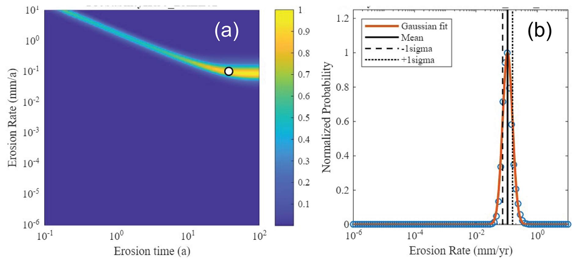
Figure 4 (a) The normalised probability likelihood surface plot of $\dot{\mathit{\epsilon }}$–t_s 10⁴ pairs in log-space for the sample IR50_BALL02. The light greenish-blue shaded sloped portion points towards a mildly fitting possible transient-state solution. The yellow-shaded patch represents the possible steady-state solutions. The white-filled circle defines the minimum t_ss. (b) The Gaussian distribution of ${\dot{\mathit{\epsilon }}}_{\text{ss}}$ for t_ss=38 a. The blue circles define the normalised values of probability likelihood of the erosion rate column of t_ss and fitted with a Gaussian distribution function. The solid, dotted and dashed black line represent the mean, +δ and −δ, respectively.

4 Performance of CoRSEER

We tested all three modules of CoRSEER for the natural data available in the literature (Lehmann et al., 2019a, b; Brill et al., 2021; Smedley et al., 2021; Luo et al., 2022; Balco et al., 2023) to: (i) benchmark the app's in-built parameters for performance, accuracy, and flexibility, and (ii) to understand how CoRSEER's mathematical framework and algorithmic implementation influence the final result. We derive three sets of outputs: (i) calibration parameters ($\stackrel{\mathrm{‾}}{\mathit{\sigma }{\mathit{\phi }}_{\mathrm{0}}}$ and μ) for the calibration samples of Lehmann et al. (2019a, b), Brill et al. (2021), Smedley et al. (2021), Luo et al. (2022), and Balco et al. (2023) using CoRSEER-I; (ii) apparent ages (t_app) for Smedley et al. (2021), Brill et al. (2021), Lehmann et al. (2019b), and Luo et al. (2022) using CoRSEER-II, because no usable unknown age LDP was available for the remaining datasets; and (iii) erosion rates for Smedley et al. (2021) and Lehmann et al. (2019b), using CoRSEER-III, because both studies have a well-established dataset of erosion history. The complete methodology for deriving the required parameters is provided in Sect. 3. We must note that all operations were performed using the FOK model (r=1), as the literature data were previously analysed using FOK. However, CoRSEER has the flexibility to use r>1, which is important when luminescence depth profiles are derived using feldspar IRSL, which follows non-FOK behaviour.

4.1 Calibration

Across the published calibration datasets, CoRSEER-I generally reproduces literature calibration parameters, with the best agreement observed for Lehmann et al. (2019a) and Luo et al. (2022), where the CoRSEER-I-derived ${\log }_{\mathrm{10}}\left(\stackrel{\mathrm{‾}}{\mathit{\sigma }{\mathit{\phi }}_{\mathrm{0}}}\right)$ and μ values are broadly comparable to reported estimates. This agreement is consistent with a similar normalisation choice for the $L_x/T_x$ depth profiles. In contrast, several datasets show systematic offsets between CoRSEER-I and the literature values. For example, in Balco et al. (2023), the sample IR50_KAY_110, the calibration parameters shift to higher values, from ${\log }_{\mathrm{10}}\left(\stackrel{\mathrm{‾}}{\mathit{\sigma }{\mathit{\phi }}_{\mathrm{0}}}\right)=-\mathrm{7.30}$ and μ=0.34 mm⁻¹ to −6.58 and 0.51 mm⁻¹ whereas for the sample pIRIR225_KAY_110 shifts to lower values, from −7.68 and 0.54 mm⁻¹ to −7.77 and 0.36 mm⁻¹. In Brill et al. (2021), CoRSEER-I predicted decreased calibration parameters for IR50_HAR1-1_CAL but increased parameters for IR50_TEM3-1_CAL and IR50_VAL4-1_CAL1. For the two calibration samples for which Brill et al. (2021) did not report the final parameters (IR50_RAB5-1_CAL and IR50_VAL4-1_CAL2), CoRSEER-I yielded −7.38, 0.76 mm⁻¹ and −7.50, 0.37 mm⁻¹, respectively. In Smedley et al. (2021), the ROAD set was dominated by a decrease in both parameters, with two clear increased cases (IR50_ROAD01 and IR50_ROAD03). The Lehmann et al. (2018) dataset shows predominantly decreased parameters for MBMB samples, with one increased case (IR50_MBMV7) and one near-balanced case (IR50_MBMV1). We attribute these discrepancies primarily to (1) differences in the fitting strategy, (2) differences in the $L_x/T_x$ normalisation (manual plateau selection versus automated normalisation) and (3) both the $\stackrel{\mathrm{‾}}{\mathit{\sigma }{\mathit{\phi }}_{\mathrm{0}}}$ and μ may slightly covary during optimisation of the best fitting. The boundary ranges of ${\log }_{\mathrm{10}}\left(\stackrel{\mathrm{‾}}{\mathit{\sigma }{\mathit{\phi }}_{\mathrm{0}}}\right)$ and μ values predicted by CoRSEER-I are −8.41 to −4.82 and 0.36 to 3.36 mm⁻¹ (Table 2), showing the plausible flexibility of the app for a wide variety of exposure conditions and lithologies.

Table 2 Comparison of model parameters of samples in the selected studies and estimated using CoRSEER-I.

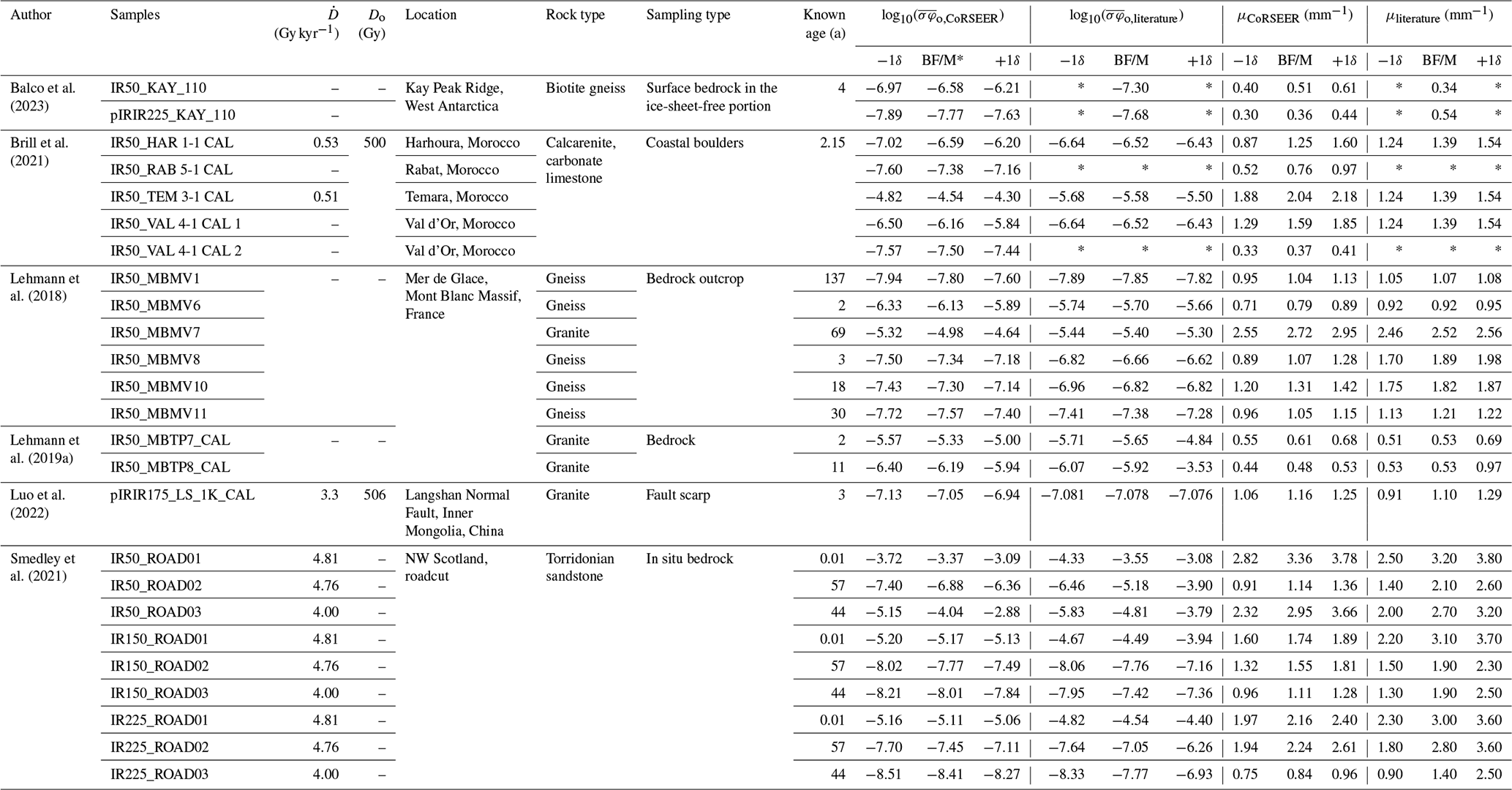
BF/M denotes the best-fit or median value; * denotes a value or uncertainty bound not reported in the cited study.

We plotted CoRSEER-I vs. the literature dataset and evaluated the R² value with respect to the 1:1 line to summarise the compilation-scale performance for 23 samples. In Fig. 5a, μ_CoRSEER versus μ_literature gives $R_{\mathrm{1}:\mathrm{1}}^{\mathrm{2}}=\mathrm{0.562}$ for n=23, meaning CoRSEER-I tracks published μ values moderately well, even though a large fraction of points falls below the 1:1 line. In Fig. 5b, ${\stackrel{\mathrm{‾}}{\mathit{\sigma }{\mathit{\phi }}_{\mathrm{0}}}}_{\text{CoRSEER}}$ versus ${\stackrel{\mathrm{‾}}{\mathit{\sigma }{\mathit{\phi }}_{\mathrm{0}}}}_{\text{literature}}$ gives $R_{\mathrm{1}:\mathrm{1}}^{\mathrm{2}}=\mathrm{0.316}$ for n=23, showing weaker agreement and stronger scatter. It is well established that the ${\stackrel{\mathrm{‾}}{\mathit{\sigma }\mathit{\phi }}}_{\mathrm{0}}$ and μ covary, and we present the relationship between them in Sect. S5 in the Supplement. To investigate the offset between the established calibration parameters and the underlying reason behind it, we plot $\left({\log }_{\mathrm{10}}\right(\stackrel{\mathrm{‾}}{\mathit{\sigma }{\mathit{\phi }}_{\mathrm{0}}})/\mathit{\mu }{)}_{\text{CoRSEER}}$ vs. $\left({\log }_{\mathrm{10}}\right(\stackrel{\mathrm{‾}}{\mathit{\sigma }{\mathit{\phi }}_{\mathrm{0}}})/\mathit{\mu }{)}_{\text{literature}}$ in Fig. 5c which gives $R_{\mathrm{1}:\mathrm{1}}^{\mathrm{2}}=\mathrm{0.379}$ showing weaker agreement. This suggests that covariance contributes only weakly to the offset, whereas normalisation and fitting strategy are the dominant contributors. Visually, most points fall below the 1:1 line in both panels, so the dominant overall tendency in this compilation is that CoRSEER estimates lower μ and $\stackrel{\mathrm{‾}}{\mathit{\sigma }{\mathit{\phi }}_{\mathrm{0}}}$ than those reported in the literature for many samples, while a smaller set of samples shows the opposite paired behaviour.

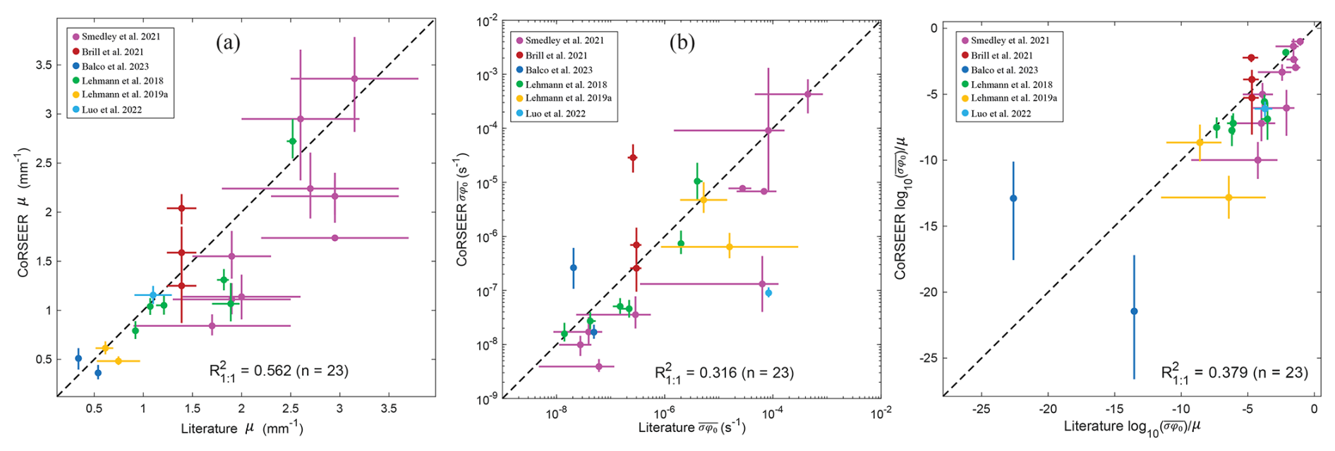
Figure 5 The 1:1 comparison between CoRSEER-I and literature calibration parameters. The round filled circles show the median/best fitting values, and the solid lines represent the respective ±δ values, which are plotted along with the black dotted 1:1 correlation line. (a) Attenuation coefficients (μ) (b) bleaching rates (${\stackrel{\mathrm{‾}}{\mathit{\sigma }\mathit{\phi }}}_{\mathrm{0}}$) and (c) the ratio ${\log }_{\mathrm{10}}\left(\stackrel{\mathrm{‾}}{\mathit{\sigma }{\mathit{\phi }}_{\mathrm{0}}}\right)/\mathit{\mu }$ for all compiled calibration samples (n=23).

4.2 Exposure age

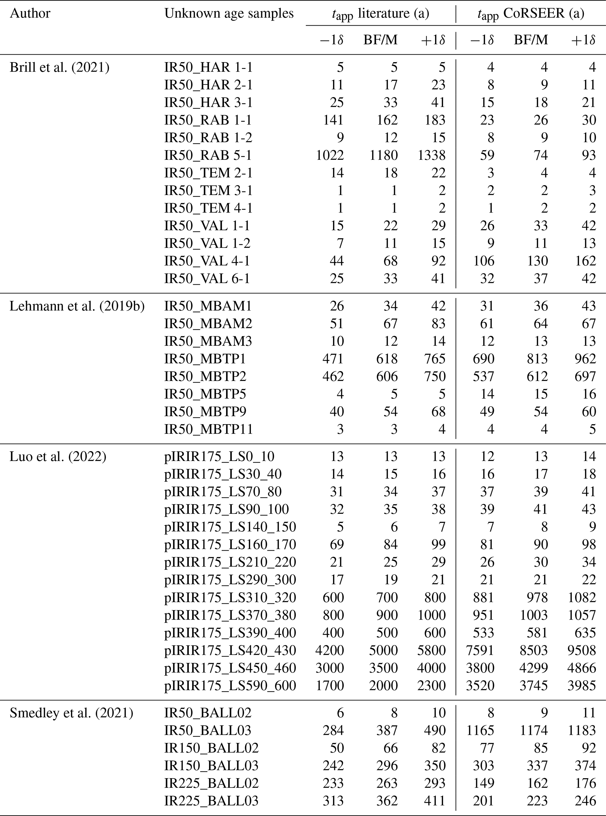
We evaluated the apparent exposure ages (t_app) of the unknown age LDPs of the literature dataset using CoRSEER-II for 41 samples. As the evaluated age exclusively depends on the chosen calibration samples, dose rate, and characteristic dose, we follow the same pattern as given in the literature dataset (unknown-age LDPs), except for a few, as mentioned further. Lehmann et al. (2019b) used a combined calibration parameter of IR50_MBTP7_CAL (2 a) and IR50_MBTP8_CAL (11 a), whereas the CoRSEER-I supports only a single calibration sample. Thus, we used IR50_MBTP7_CAL, as it closely resembles the calibration parameters in the literature. For Brill et al. (2021), we used CoRSEER-I to evaluate the parameters of IR50_RAB 5-1 CAL for the samples of IR50_RAB 1-1, IR50_RAB 1-2, and IR50_RAB 5-1 (these samples were evaluated using IR50_HAR 1-1 CAL in the literature due to the large uncertainty in IR50_RAB 5-1 CAL). We plotted the CoRSEER-II derived versus published literature apparent age dataset and evaluated the $R_{\mathrm{1}:\mathrm{1}}^{\mathrm{2}}$ value with respect to the 1:1 line to summarise the compilation-scale performance. Interestingly, the evaluated t_app using CoRSEER-II is comparable to the literature and falls closely around the 1:1 line (Fig. 6) despite a significant difference in the calibration parameters used in this study. The derived $R_{\mathrm{1}:\mathrm{1}}^{\mathrm{2}}=\mathrm{0.889}$ represents the CoRSEER-II track, which has apparent exposure ages with high certainty. There was a significant underestimation by CoRSEER-II for the IR50_RAB 1-1, IR50_RAB 5-1 and IR50_TEM 2-1. This is due to the following reasons: (1) a change in the calibration sample, as mentioned earlier. (2) The high SCF normalisation factors a=1.1 (up to 10 %) of the sigmoidal fitting for the IR50_TEM 2-1, which might have changed the position of x_0.5.

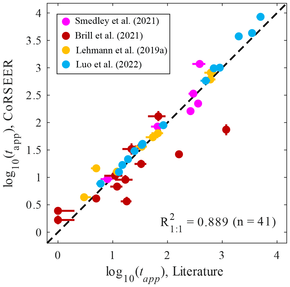
Figure 6 The 1:1 comparison between CoRSEER-II and literature t_app data. The round filled circles show the median/best fitting values, and the solid lines represent the respective ±δ values, which are plotted along with the black dotted 1:1 correlation line.

The range of t_app values predicted by CoRSEER-II extends from 1 a to 8.5 ka (Table 3), showing its potential as a decadal-to-millennial chronometric mathematical tool for LRSED.

Table 3 Representation of exposure ages for samples evaluated from both the literature and CoRSEER.

4.3 Erosion rates

Here, we establish the steady-state erosion rate (${\dot{\mathit{\epsilon }}}_{\text{ss}}$) and corresponding onset time of erosion (t_ss) of literature dataset (n=11) using CoRSEER-III. We carefully chose the calibration and dose parameters, as mentioned in the earlier sections. The choice of sample for analysis assumes that these samples are in a steady state, as described in the literature (Lehmann et al., 2019a; Smedley et al., 2021). Comparison of the literature and CoRSEER-derived erosion rates is important because, unlike the previous studies, CoRSEER-III derives erosion rates directly from the ${\dot{\mathit{\epsilon }}}_{\text{ss}}$–t_ss matrix. Therefore, the present result is not only a comparison with previously reported values, but also the first systematic demonstration of an algorithmic method for extracting erosion-rate solutions from this matrix. The results are shown in Table 4.

Table 4 Representation of steady-state onset exposure age and erosion rates for samples evaluated from both the literature and CoRSEER-III.

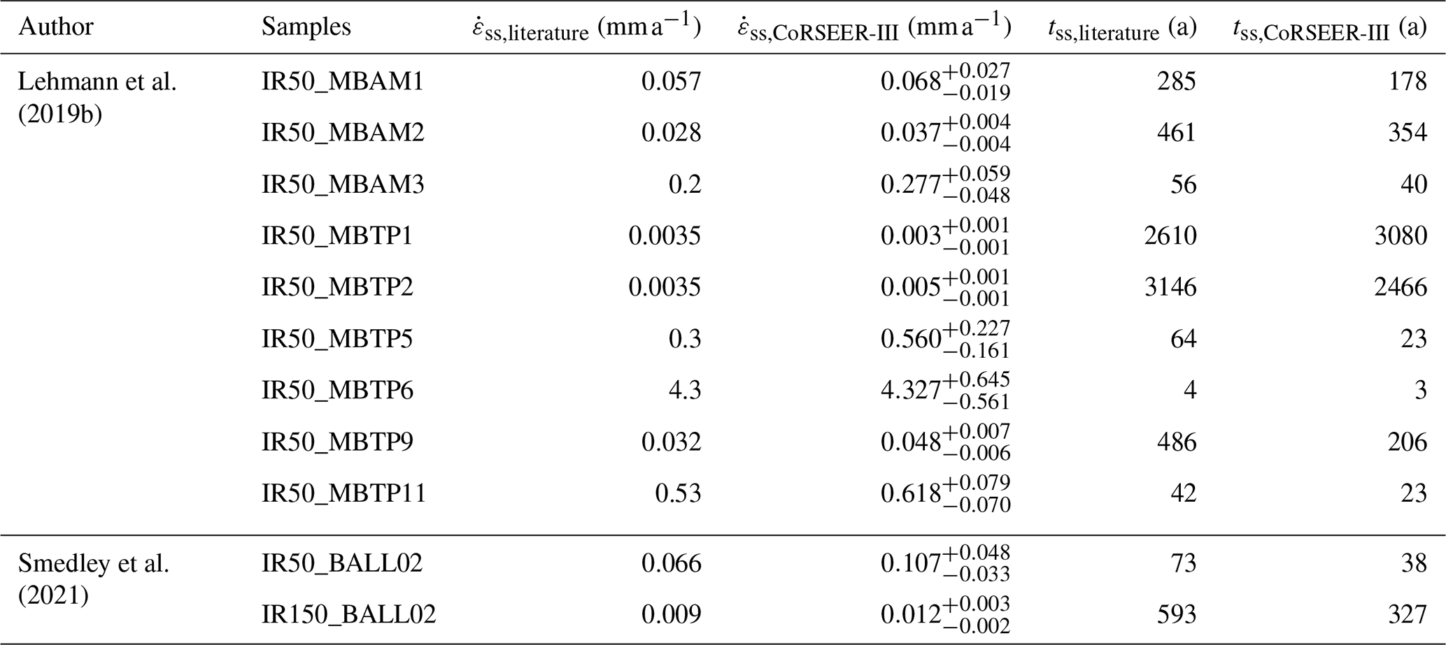
The CoRSEER-III-derived erosion rates broadly agree with the literature erosion-rate values. The literature erosion rates range from 0.0035 to 4.3 mm a⁻¹, whereas the CoRSEER-III-derived erosion rates range from 0.003 to 4.327 mm a⁻¹. Using the literature values as reference, the absolute percentage difference ranges from 0.6 % to 86.7 %. The minimum difference occurs for IR50_MBTP6, where CoRSEER-III gives 4.327 mm a⁻¹ compared with the literature value of 4.3 mm a⁻¹. The largest difference occurs for IR50_MBTP5, where CoRSEER-III gives 0.560 mm a⁻¹ compared with the literature value of 0.300 mm a⁻¹.

The uncertainty associated with CoRSEER-III-derived erosion rates remains within a reasonable range for most samples. The relative upper error in the CoRSEER-III erosion rates varies from 10.8 % to 44.9 %, whereas the relative lower error varies from 10.8 % to 33.3 %. The lowest relative uncertainty occurs for IR50_MBAM2, where the erosion rate is 0.037 mm a⁻¹ with an uncertainty of approximately ±10.8 %. The highest upper uncertainty occurs for IR50_BALL02, where the upper error reaches approximately 44.9 %. These values show that the algorithm provides bounded erosion-rate estimates rather than single manually selected solutions.

In contrast, the erosion-onset time, t_ss, shows a considerably larger departure from the literature values. The literature t_ss values range from 4 to 3146 a, whereas the CoRSEER-III-derived t_ss values range from 3 to 3080 a. Using the literature values as reference, the absolute percentage difference ranges from 18.0 % to 64.1 %. In most samples, CoRSEER-III estimates a younger erosion-onset time than the literature value. The only exception is IR50_MBTP1, where CoRSEER-III gives a larger onset time of 3080 a compared with the literature value of 2610 a, corresponding to an increase of approximately 18.0 %. The maximum difference occurs for IR50_MBTP5, where CoRSEER-III estimates 23 a compared with the literature value of 64 a, corresponding to a reduction of approximately 64.1 %.

Overall, the results indicate that CoRSEER-III reproduces the erosion-rate field reasonably well, as presented in Table 4, but it estimates erosion-onset time differently from the literature. This difference is expected because the CoRSEER-III estimate is derived from an automated best-fitting erosion-time slope detection algorithm, whereas previous studies relied more strongly on manual or interpretative selection of model solutions.

When the sample is in a transient state, one can visually identify the solution that generally lies in the sloped portion of the ${\dot{\mathit{\epsilon }}}_{\text{ss}}$ vs. t_ss likelihood plot. It is mathematically challenging to produce an objective method to constrain a pair of possible solutions. Thus, we do not present any transient-state condition scenarios. But it is possible to derive a transient state solution from the results of CoRSEER-III if the onset of erosion (t_s) is known by some means.

5 Discussion

The LRSED is a promising chronometer of geological processes which occur under sufficient sunlight. Rigorous methodological development and precise field application of LRSED can cause a paradigm shift in surface exposure chronometry by enabling us to date decadal to millennial exposure events. Furthermore, it can accurately establish steady-state in situ erosion rates. Although this method is affected by broader challenges such as the availability of calibration samples, representative luminescence depth-profile selection, lithological suitability, and independent exposure-age constraints, additional methodological uncertainty can arise from subjective plateau selection and the use of non-standardised modelling approaches. Thus, CoRSEER attempts to improve the application, standardisation, and intercomparison of results among several studies.

5.1 Preliminary precautions

Large scatter in the luminescence depth profile (LDP) and high fractional uncertainty in $L_x/T_x$ make plateau identification unreliable and reduce the stability of any inversion (i.e., the SCF normalisation, estimation of calibration parameters, exposure age, erosion rates). We can reduce $L_x/T_x$ uncertainty by adopting a modified post-infrared infrared stimulated luminescence protocol with lower heating rates and longer isothermal holding times (Jenkins et al., 2018), and by using metal cups (Elkadi et al., 2021). For each sample, we recommend measuring two or more LDPs and maintain millimetre-scale sampling density with a substantial fraction of points located on the sigmoidal transition. Importantly, the fractional error structure should be similar or random with depth; if the fractional error at lower depths is systematically higher than at higher depths, the fitting becomes biased toward the plateau, and the inferred parameters become unreliable. Although we cannot yet provide a statistical criterion for the required fraction of points on the sigmoidal part of the curve, based on our observation in Figs. 2a and 3a, we recommend that more than 50 % of all $L_x/T_x$ measurement points should lie before the final plateau. If the measured profile is dominated by plateau points, we recommend reducing the measurement depth such that the total number of points on the initial plateau and sigmoidal region exceeds 50 % of the total.

In the case of incomplete LDP, the maximum measurement depth is shallower than the steady-state depth, the plateau cannot be reconstructed. We therefore recommend measuring $L_x/T_x$ up to the equilibrium depth (which is the stable plateau). Similarly, for the large scatter in experimental data, it is difficult to identify the plateau manually. The SCF and parameter estimation to normalise the LDP is a major step forward as it resolves both issues and removes the manual intervention from mathematical inversion, thereby improving the accuracy of fitting (Fig. 2e).

5.2 Calibration

While using CoRSEER-I, we suggest that there are a few precautions we must take to estimate ${\stackrel{\mathrm{‾}}{\mathit{\sigma }\mathit{\phi }}}_{\mathrm{0}}$ and μ accurately. If the IRSL signal from feldspar minerals is used for LDP measurements, we suggest evaluating the order of kinetics (r) beforehand and incorporating it into the calculation. The application of FOK can cause severe underestimation and overestimation of the exposure age and erosion rate (Biswas et al., 2023; Pathan et al., 2024). The different methods for evaluating the r value are thoroughly discussed in Biswas et al. (2023) and Pathan et al. (2024). Furthermore, if the calibration sample is young (say 1–10 a), for example, a known-age deglaciated surface or manually exposed surface created by chipping off a boulder face, erosion is assumed to have no effect on the LDP. In contrast, when using older natural calibration samples (t>100 a), erosion is expected to affect LDP significantly (Lehmann et al., 2018; Smedley et al., 2021), and this effect becomes stronger in high-erosion environments. This can lead to substantial underestimation of ${\stackrel{\mathrm{‾}}{\mathit{\sigma }\mathit{\phi }}}_{\mathrm{0}}$ and smaller bias in μ. This is inferred from the samples IR50_MBMV1 (t=137 a) and IR50_MBMV6 (t=2 a), which were samples from the same site with similar lithology, but the $\log {\stackrel{\mathrm{‾}}{\mathit{\sigma }\mathit{\phi }}}_{\mathrm{0}}$ was estimated as −7.8 and −6.13, respectively, which is a difference of about two orders of magnitude, whereas μ was estimated at 1.04 and 0.8 mm⁻¹. Thus, the erosion rate must be explicitly incorporated into CoRSEER-I. To avoid this complexity and reduce model dependence on uncertain erosion histories, it is recommended to use young calibration surfaces at sampling sites where there is no erosion over the period of interest. This allows for the precise calibration of kinetic parameters under well-constrained exposure conditions. This will further remove any ambiguity due to changes in decay kinetics, lithology, surface orientation, shielding, and light penetration.

When selecting a calibration sample, it is critical to recognise that the light attenuation coefficient (μ) and the effective detrapping rate at the surface ($\stackrel{\mathrm{‾}}{\mathit{\sigma }{\mathit{\phi }}_{\mathrm{0}}}$) of the calibration samples are the best representatives of the actual sample. Recent empirical studies demonstrate that photon penetration and attenuation are highly sensitive to micro-mineralogical heterogeneity, such as the spatial distribution of opaque and translucent minerals, which can cause localised “light piping” or “shadowing” (Meyer et al., 2018; Cui et al., 2024). Furthermore, μ is strongly wavelength-dependent and can be drastically altered over time by dynamic surficial boundary conditions, including the accretion of rock varnish (Luo et al., 2018) or localised iron-hydroxide precipitation due to moisture (Meyer et al., 2018; Smedley et al., 2021). The effective detrapping rate ($\stackrel{\mathrm{‾}}{\mathit{\sigma }{\mathit{\phi }}_{\mathrm{0}}}$) is similarly sensitive to external environmental geometries, fluctuating significantly based on the target surface's topographic aspect, inclination, and seasonal solar incidence angles (Fuhrmann et al., 2022). High-resolution spatial analyses reveal that these optical properties can vary significantly even on a sub-millimetre scale within contiguous rock formations (Ou et al., 2018; Smedley et al., 2025). Consequently, to avoid severe systematic chronological errors, it is imperative to ensure that the optical characteristics, dynamic surficial coatings, and spatial orientation governing μ and $\stackrel{\mathrm{‾}}{\mathit{\sigma }{\mathit{\phi }}_{\mathrm{0}}}$ in the calibration sample, the measurements are meticulously matched to those of the unknown target sample.

Although our present modelling framework focuses on single calibration (SC), it is worth noting that multi-calibration strategies (MC) can be highly effective under certain conditions. When multiple calibration samples of different known ages, but from the same lithology and sunlight exposure conditions, are available, it becomes possible to constrain ${\stackrel{\mathrm{‾}}{\mathit{\sigma }\mathit{\phi }}}_{\mathrm{0}}$, μ and r simultaneously (Pathan et al., 2024). However, the accuracy of such multi-calibration depends strongly on the number of calibration samples and their age spread. A wider temporal distribution across well-characterised surfaces enhances the resolution of the kinetic behaviour. While we recognise the potential of this methodology, it lies beyond the scope of the current work and is not implemented in the present version of CoRSEER.

5.3 Apparent age estimation

After estimation of kinetic parameters, the estimation of exposure and erosion history appears to be highly dependent on the position of x_0.5. There are two possible scenarios:

Case 1: For non-eroding exposure conditions, if the depth of half saturation of the LDP, x_0.5 is smaller than x_0.5,max, then the apparent exposure age is equal to the actual exposure age of the sample, and if $x_{\mathrm{0.5},\text{max}}<x_{\mathrm{0.5}}\le x_{\mathrm{0.5},\text{ss}}$ then the sample reaches steady-state, and the exposure age is greater than the t_max, maximum dateable exposure age.

Case 2: If the derived apparent ages are substantially lower than the expected age (derived using an independent method), this indicates the presence of erosion, which was seen in the sample IR50_BALL02 (Smedley et al., 2021). CoRSEER-III should be used to further re-establish the exposure-erosion history. Furthermore, when using IRSL to establish the LDP, the r value should be the same for calibration and unknown samples (Pathan et al., 2024). We incorporated all these modelling aspects, diagnostics, and interpretation into the input and output GUI plots (Fig. 3).

5.4 Erosion rate estimation

The fundamental assumptions and modelling aspects underpinning CoRSEER-III were taken from Lehmann et al. (2019a), where the authors coupled ¹⁰Be concentration and the LDP to evaluate the erosion-corrected ¹⁰Be exposure age range. The main difference is that CoRSEER-III does not incorporate ¹⁰Be concentration; rather, it incorporates independent exposure age (i) which can be derived from an independent dating method or (ii) by incorporating t_max from forward modelling of x_0.5 vs. t.

One of the most important observations is that CoRSEER-III captures the same broad erosion-rate scale as the literature values. This indicates that the erosion-rate extraction algorithm is able to preserve the first-order structure of the erosion solution space. In practical terms, this is encouraging because the algorithm avoids subjective manual picking while still recovering erosion-rate estimates comparable to previous studies. This is also a possible reason for the large relative difference between CoRSEER and literature results in a few cases. Thus, for maximum accuracy and precision, we recommend following the guidelines. Users should not run the model once over a very large erosion-exposure window and treat the result as final. A better strategy is to run the model in multiple stages. First, use a broad search window to identify the approximate high-likelihood region. Then shrink the exposure-erosion window around that region. Finally, increase the matrix density so that the best-fitting slope is resolved with higher numerical precision. This stepwise refinement should reduce grid artefacts and improve the stability of both erosion-rate (and errors) and onset-time estimates.

6 Conclusion

In this study, we present CoRSEER as an integrated, reproducible workflow for LRSED that converts the LDP into physically interpretable exposure and erosion information. CoRSEER reduces user-dependent choices by automating key steps that vary across studies. CoRSEER comprises three linked modules: (i) calibration of site- and lithology-specific bleaching parameters, (ii) apparent exposure age estimation, and (iii) erosion rate estimation under steady-state scenarios. Reanalysis of published datasets shows that CoRSEER-I generally reproduces plausible calibration parameter estimates and captures literature trends, while also presenting systematic offsets in some datasets that mainly arise from differences in normalisation and fitting strategy. Despite these calibration differences, CoRSEER-II yields apparent exposure ages that closely track published values with strong 1:1 agreement, demonstrating that the platform provides robust chronometric outputs when calibration inputs are selected consistently with the reference studies. Finally, CoRSEER-III reproduces steady-state erosion histories with excellent agreement for well-constrained erosion datasets, supporting its use as a quantitative erosion-rate estimator when exposure age constraints are available, and the profile indicates steady-state behaviour. These results support the central conclusion that objective normalisation and standardised inversion materially improve reproducibility in LRSED without reducing model flexibility. CoRSEER enables consistent decadal-to-millennial exposure reconstructions and strengthens its practical use, but there are a few limitations which must be addressed. The CoRSEER's performance depends on data quality; that is, a significant number of $L_x/T_x$ samples across the sigmoidal slope and lesser $L_x/T_x$ error estimates remain essential, and shallow or plateau-dominated profiles can bias sigmoidal fitting. The current release prioritises single-sample calibration and does not yet implement multi-calibration optimisation, and the objective selection of transient-state erosion solutions remains mathematically challenging and therefore user-guided. Future versions should (i) implement multi-calibration strategies to constrain kinetic parameters jointly, (ii) expand diagnostics that flag profiles likely to be poorly constrained, and (iii) develop a similar GUI framework for luminescence rock surface burial dating.

Appendix A: Symbology, units, and descriptions of parameters used

Symbol	Unit	Description
n	Dimensionless	Number of trapped electrons
N		Maximum possible number of trapped electrons
$\stackrel{\mathrm{‾}}{n}$	dimensionless	Normalised electron trap population
${\stackrel{\mathrm{‾}}{n}}_{\text{sim}}$		Simulated normalised luminescence signal
${\stackrel{\mathrm{‾}}{n}}_{\text{obs}}$		Natural normalised luminescence signal
σ	mm2	Luminescence photoionisation cross section
φ0	${\mathrm{mm}}^{-\mathrm{2}}{\mathrm{s}}^{-\mathrm{1}}$	Photon flux on the surface of the rock
$\stackrel{\mathrm{‾}}{\mathit{\sigma }{\mathit{\phi }}_{\mathrm{0}}}$	s−1	Wavelength-dependent luminescence decay constant of rocks
μ	mm−1	Attenuation coefficient
$\dot{D}$	Gy a−1	Environmental dose rate
D0	Gy	Characteristic dose of saturation (Dose that fills ∼63 % of the traps) (Wintle and Murray, 2006)
r	dimensionless	Order of kinetics (Biswas et al., 2023; Freiesleben et al., 2023)
Lx	counts s−1	The luminescence intensity of the natural sample
Tx	counts s−1	The luminescence intensity of the laboratory-dosed sample
$L_x/T_x$	dimensionless	The laboratory-dose normalised luminescence intensity for the natural sample
a	dimensionless	Upper asymptote, the maximum value the function can attain when x approaches infinity
b	mm−1	Steepness of the curve or growth rate of the curve
c	mm	Depth of the inflection point, also referred to as x0.5
χ2	dimensionless	Chi-square
Pk		Likelihood value associated with the synthetic LDP numbered as k
Pmax		Maximum likelihood, which is associated with the best-fitting synthetic LDP
$P_{\text{norm}}^k$		Normalised likelihood value associated with the synthetic LDP numbered as k
δ		Standard deviation
α		Fractional error, which is equal to $(L_x/T_x)/(L_x/T_x{)}_{\text{error}}$
R2		Coefficient of determination
x	mm	Depth from surface
x0.5		Depth of half saturation from the surface
x0.5,max		Forward modelled half saturation depth associated with the maximum detectable age limit.
x0.5,ss		Forward-modelled half-saturation depth when the LDP is in a steady state and purely acts as an erosion meter.
x0.5,natural		Half saturation depth for natural LDP also equals the c value.
t	a	Exposure age
tmax		Maximum age limit for the samples
ti		Independent exposure age by any other method
tcal		Known exposure age of calibration sample
ts		Onset time of erosion
tss		Steady-state erosion time
tapp		Apparent exposure age
$\dot{\mathit{\epsilon }}$	mm a−1	Erosion rate
${\dot{\mathit{\epsilon }}}_{\text{ss}}$		Steady-state erosion rate