Technical note: T_c1D – a 1D thermal and thermochronometer age prediction model

Thermochronological data are commonly used to study the activity of geological processes over timescales of millions of years. Ages produced by thermochronological measurements, however, are non-unique and do not directly record rates of processes, which has led to the development of a variety of software tools for interpreting age data in the context of geological processes. Most of the widely used software packages focus on determining thermal histories, which are easy to use but do not provide direct quantitative estimates of geological process rates. In contrast, more sophisticated and complex thermo-kinematic modeling software can link ages to process rates but may require greater computational expertise and resources for use. Here we introduce T_c1D, a 1D thermal and thermochronometer age prediction software package designed to provide users with the opportunity to explore geological processes from thermochronology data in a computationally efficient and accessible framework. The software is open source and written in the Python programming language, and provides functionality for forward and inverse modeling of thermochronometer data, visualization using built-in plotting, a variety of options for defining exhumation histories, and more. This work presents an overview of how T_c1D was designed, several illustrative examples of how the code can be applied, instructions for how to get started using T_c1D, and some plans for future development.

1 Introduction

Thermochronology data provide a record of the thermal history of rocks over timescales from 10⁵–>10⁸ years (e.g., Reiners et al., 2005). This record, however, can be difficult to establish from the age data alone due to the non-unique nature of thermochronometer ages. Thus, numerical modeling software is frequently used to robustly constrain the timing and magnitude of cooling (or heating), i.e., a rock's thermal history (e.g., Reiners and Brandon, 2006; Fox and Shuster, 2020; McDannell and Flowers, 2020). Such software often uses thermochronometric ages in combination with other measurements (e.g., fission track length distributions or noble gas diffusion profiles) or geological data (known thermal constraints such as times of surface exposure) to identify probable thermal history ranges through data inversion. While these thermal histories can provide valuable information about the timing of temperature changes in rocks over those timescales, a primary goal in thermochronology studies is to relate thermal histories to the tectonic, erosional, hydrothermal, and/or magmatic processes that produced the thermal response (e.g., Ehlers, 2005; Malusà and Fitzgerald, 2019; Gautheron et al., 2022), which can be challenging. In such cases, not only are constraints on the thermal history needed, but so is some representation of the dynamic evolution of the crustal thermal field over the duration of that thermal history (e.g., Ehlers, 2005).

Numerous software packages have been developed in the thermochronology community for calculating both thermal and exhumation histories from thermochronometer data. While several available thermal history modeling software packages are user friendly, those designed for calculating exhumation histories may have important limitations or require computational skills and resources that limit their potential generalized use. The most widely used thermal history modeling software packages are HeFTy (Ketcham, 2005) and QTQt (Gallagher, 2012), which feature support for numerous different thermochronometers and associated kinetic models, and have mature graphical user interfaces and features that make them easy to use for researchers without extensive backgrounds in scientific computing. Differences exist in the approaches used to determine plausible thermal histories (see, for example, Fox and Carter, 2020; Murray et al., 2022; Abbey et al., 2023, or Vermeesch and Tian, 2014, and subsequent comments and replies), but both utilize input age data, related measurements such as fission track length distributions, and thermal history constraints from geological observations to delineate possible thermal histories that are consistent with the measured ages. However, neither package is open source, and only limited information about possible rates of exhumation can be inferred from the derived thermal histories (e.g., Fig. 1). Thermochron.jl (Keller et al., 2022) is an open-source software package similar in many ways to QTQt, with the advantage that the source code is available to aid users in understanding details about how the software operates. However, Thermochron.jl calculates thermal histories only, and is thus still limited in the user's ability to infer past geological processes, or rock exhumation histories.

Figure 1 Power of different thermochronometer data modeling software packages to infer geological processes as a function of their ease of use. References: ¹ Ketcham (2005), ² Gallagher (2012), ³ Braun (2003).

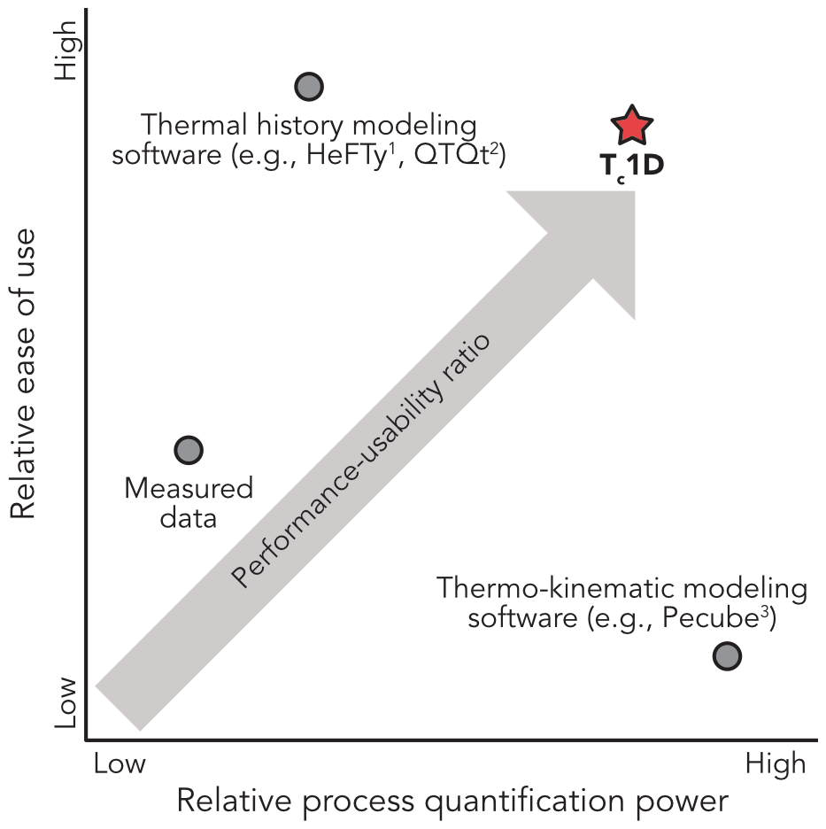
Exhumation rates from thermochronometer data can be estimated using several different software packages, each differing in computational expense and ease of use. GLIDE (Fox et al., 2014) uses a linear inversion approach with 1D thermal models to estimate spatial and temporal variations in exhumation rates from low-temperature thermochronometer age datasets of ten or more ages. This powerful approach is, however, not suitable for samples that record burial or reheating. Another easy-to-use software tool is age2exhume (van der Beek and Schildgen, 2023), which is also suitable for large thermochronometer datasets. age2exhume, inspired by the earlier age2edot software (Brandon et al., 1998; Willett and Brandon, 2013), uses an iterative approach to determine spatially variable best-fit exhumation rates for thermochronometer datasets, including the effects of topography and elevation on the thermal histories generated using a 1D thermal model. The key limitations for age2exhume, are that the calculated best-fit exhumation rates cannot vary with time and Dodson's approach (Dodson, 1973) is used for calculating effective closure temperatures, rather than more sophisticated age prediction algorithms that include the effects of radiation damage on calculated ages (e.g., Flowers et al., 2009; Guenthner et al., 2013). For simulating the thermal effects of geological processes in 3D and determining corresponding exhumation histories, the most broadly used software is Pecube (Braun, 2003; Braun et al., 2012), which is a thermo-kinematic numerical modeling package that has the capability to model the 3D evolution of crustal temperatures, topography, rock thermal properties, and more, including the possibility for inverse modeling of thermochronometer age datasets. Pecube is thus an extremely powerful tool for determining exhumation histories from thermochronometer data, but with the drawback that use of the software requires a deeper knowledge of scientific computing, software compilation, and potentially the use of high-performance computing clusters (e.g., Fig. 1). Although some efforts are being made to make Pecube more user friendly (e.g., Bernard et al., 2025), Pecube is a tool best used by researchers with strong computational skills and access to suitable computing resources.

Here we introduce T_c1D, a software which aims to provide the thermochronologist with the possibility to link geological processes with thermochronometer age data while remaining easy to use, access, and understand (Fig. 1). T_c1D provides similar functionality to HeFTy or QTQt for inverse modeling of thermochronometer data, while fundamentally linking thermal histories to rates of exhumation, burial, magmatic heating, or other crustal thermal processes. The software uses a one-dimensional (depth) geometry, which means that it is both less complex in its design and computationally lighter than Pecube. We view this software contribution as complementary to existing tools, and explain below the fundamental design choices, operations, and illustrative examples of how T_c1D can be used to apply thermochronometric data to understand geological processes.

2 Design philosophy

T_c1D is intended for modeling fundamental processes that influence thermochronometers, with a software package that is designed to be both easy to use and flexible. The core operations included in T_c1D comprise: 1D thermal modeling, recording thermal histories of exhumed tracking particles, and thermochronometer age prediction using the recorded thermal histories. The thermal model (described in more detail in Sect. 3.1) calculates the evolution of temperatures in the lithosphere due to vertical transport of heat by various geological processes, such as exhumation, burial, or magmatism. During temperature calculation, one or more tracking particles are used to record thermal histories as they are transported toward (or away from) the model surface, ending their transport at the model surface. The recorded thermal histories are then used to calculate thermochronometer ages for various systems, as described in more detail in Sect. 3.2. Thus, geological processes can be used to define how mass moves in the 1D vertical rock column, and the resulting thermal evolution will be used to connect these processes to thermochronometer ages.

T_c1D is an open-source software package written mainly in Python that can be used with most operating systems or an interactive coding environment. Python was chosen as the programming language for T_c1D because it is widely used (i.e., it was the most widely used programming language on GitHub.com in 2024), and is commonly taught and used in the natural, computational, and data sciences due to its ease of use and the wealth of available online Python resources (e.g., Perkel, 2025). In T_c1D, models can be run from within a Python interpreter, a Python script, or from an interactive coding application such as a Jupyter Notebook (e.g., Granger and Pérez, 2021). In these instances, various calculations in T_c1D are run by calling functions from the T_c1D package. However, it is also possible to operate T_c1D through a command-line interface. The command-line interface allows for use in the terminal as well as in shell script files, providing further flexibility. In addition to configuring T_c1D using command-line arguments, it also supports model configuration through an input file. The input file uses the YAML file format, which provides a consistent structure while remaining easily human readable. The input centralizes the definition of model parameters, which is particularly useful for simulations involving many non-default parameters or for workflows in which similar models are run repeatedly with only minor changes to the parameter values. The YAML-based input file also enhances reproducibility by making complete model designs easier to archive, share, and rerun. It complements the existing command-line interface by mirroring the available flags and parameters in an accessible format. For new users, the T_c1D documentation site and repository on GitHub.com have links that launch an interactive Jupyter environment with notebooks that introduce basic code functionality. The linked notebooks can be used from a computer, tablet, or smartphone without requiring software installation.

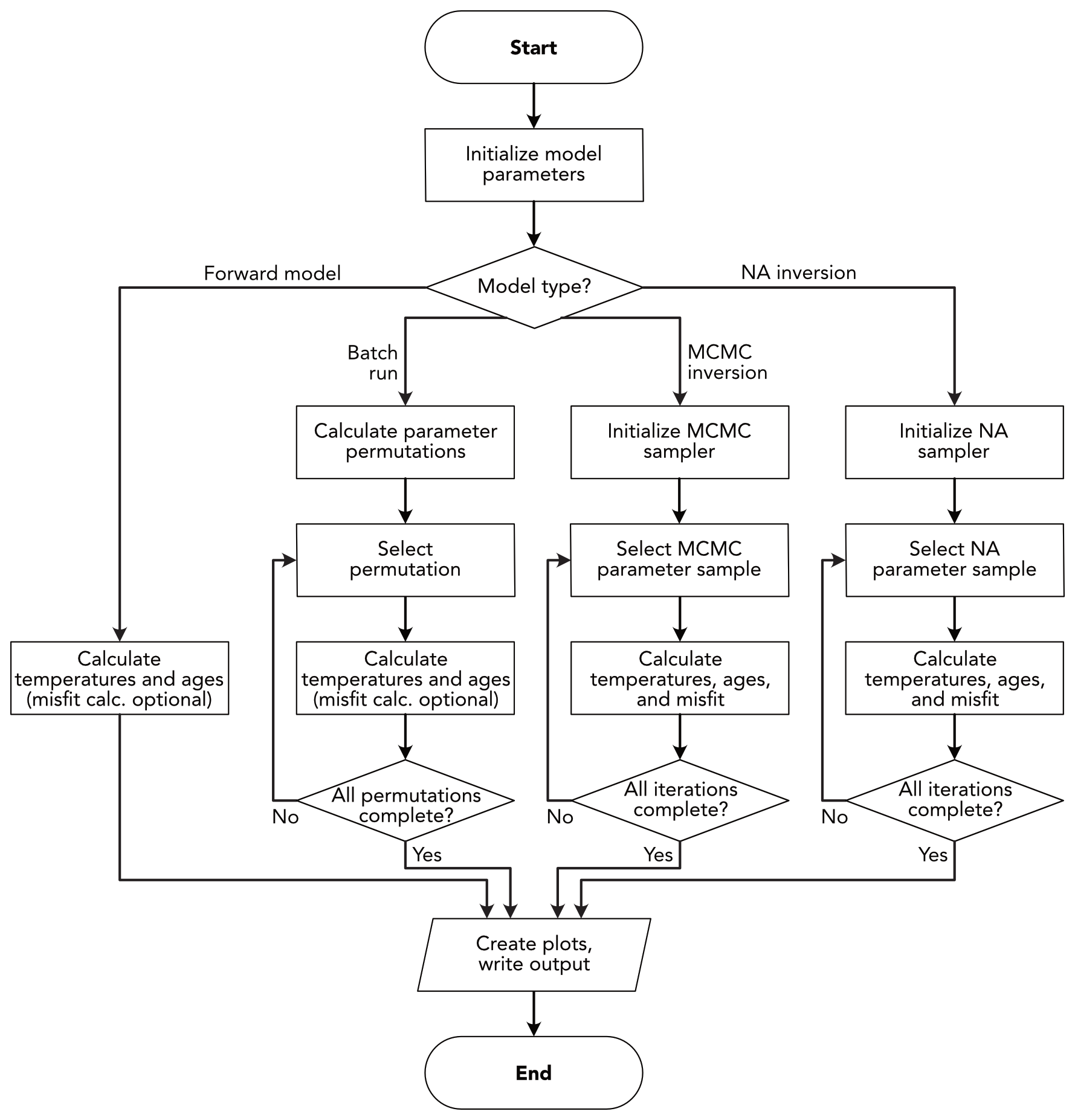
Figure 2 Flowchart of various model types in T_c1D. MCMC, Markov chain Monte Carlo; NA, Neighbourhood Algorithm.

In addition, T_c1D provides options for forward and inverse modeling to support both process exploration and data-driven studies (e.g., Fig. 2). Forward models can be useful for assessing sensitivity to various model parameters, testing various geological hypotheses, or simply exploring how ages vary for different types of burial and exhumation histories. In such cases, the user specifies a set of input parameters for a T_c1D simulation and the model outputs a series of plots depicting the evolution of temperatures in the model, particle thermal history, and predicted thermochronometer ages (see Sect. 3.1 and 3.2 for details). To utilize the inverse modeling functionality in T_c1D, users provide a set of measured thermochronometer ages in an age data file or via function parameters. In this mode, T_c1D will search within specified ranges of input parameters to identify the ranges of parameters that provide the best fits to the measured age data (e.g., Fig. 2). This approach is ideal for using a set of measured ages to determine rates of burial and exhumation, timing of various geological processes, and the impact of rock thermo-physical properties on the measured age data. More information about inverse modeling in T_c1D is given in Sect. 3.3.2.

3 Methods

3.1 Forward modeling temperature and thermal histories

Temperatures in T_c1D start from a thermal steady state and evolve forward in time as the result of heat advection, conduction, and production. The general form of the transient heat transfer equation in 1D, including the effects of advection, conduction, and heat production, is

$$\begin{array}{}\text{(1)}& \mathit{\rho }{C}_p\left({\displaystyle \frac{\partial T}{\partial t}}+v_z{\displaystyle \frac{\partial T}{\partial z}}\right)=-{\displaystyle \frac{\partial q_z}{\partial z}}+H,\end{array}$$

where ρ is rock density, C_p is rock heat capacity, T is temperature, t is time, v_z is the vertical advection velocity, z is the spatial coordinate (depth in T_c1D), and H is heat production. The vertical heat flux term is q_z, which can be calculated as

$$\begin{array}{}\text{(2)}& q_z=-k{\displaystyle \frac{\partial T}{\partial z}},\end{array}$$

where k is thermal conductivity. The time evolution of temperature in T_c1D is calculated using either an explicit or implicit finite-difference formulation of Eq. (1) using a user-defined time step dt. Heat produced by radioactive decay is currently the only heat source for the production term H, and the material properties ρ, C_p, k, and H can vary in the model crust, mantle lithosphere, and asthenospheric mantle materials. Heat production H in the crust can be constant or decay exponentially to simulate the concentration of heat-producing elements in upper crustal rocks. To ensure the heat flux is conserved across node points in the finite-difference grid, a staggered grid is used for thermal conductivity (e.g., Gerya, 2010).

Node points are fixed in space during T_c1D calculations and the evolution of temperature in the models is constrained by constant temperature boundary conditions at the surface and base of the model. The initial temperatures in T_c1D are calculated by setting the time-dependent term in Eq. (1) to zero, yielding

$$\begin{array}{}\text{(3)}& \mathit{\rho }{C}_p\left(v_z{\displaystyle \frac{\partial T}{\partial z}}\right)=-{\displaystyle \frac{\partial q_z}{\partial z}}+H.\end{array}$$

Equation (3) is solved using an implicit finite-difference formulation, and it is important to note that the initial conditions can thus include the effects of an initial advection velocity or variable material properties (including heat production). Values used to define the boundary condition temperatures are assumed to be constant over the duration of the simulation with the present version of T_c1D, however they could vary in time in principle.

Because the node points do not move in T_c1D, the vertical advection velocity v_z defined in different user-selectable erosion models affects both the model thermal field and the thermal history of tracking particles exhumed or buried during the simulation (see T_c1D documentation at https://tc1d.readthedocs.io/en/latest/erosion-models.html (last access: 30 April 2026) for an overview of available erosion models). Starting from a position at the model surface at 0 Ma, a particle's starting depth is back-calculated by running the erosion model backwards in time for the duration of the numerical experiment. The particle's position is then updated forward in time during each model time step by v_z⋅dt, and the current depth, pressure, and temperature are recorded. Depth, pressure, and thermal histories can be calculated for particles ending at the surface at the end of the numerical experiment or at various user-defined times during the experiment.

3.2 Thermochronometer age prediction and data comparison

The modeled thermal history (or histories) can be used to calculate thermochronometer ages for the (U–Th)$/$He and fission-track systems in apatite and zircon (e.g., Fig. 3). (U–Th)$/$He age prediction includes the effects of radiation damage and annealing through the RDAAM model of Flowers et al. (2009) for apatite (U–Th)$/$He (AHe) ages and the ZRDAAM model (Guenthner et al., 2013) for zircon (U–Th)$/$He (ZHe) ages. Both use an external program from Ketcham et al. (2018). Apatite fission-track (AFT) ages can be predicted either using the fission track annealing model of Ketcham et al. (1999) or that of van der Beek (1995). The Ketcham et al. (1999) model has the Cl content set to 0 ppm and uses the approach of Ketcham et al. (2000) as implemented in Braun et al. (2012). The AFT model from van der Beek (1995) can use the kinetic parameters from Laslett et al. (1987) or the Durango or fluorapatite kinetics from Crowley et al. (1991). Zircon fission-track (ZFT) age prediction uses the approach of van der Beek (1995) with the kinetics of either Tagami et al. (1998) or Rahn et al. (2004) following the implementation in Braun et al. (2012).

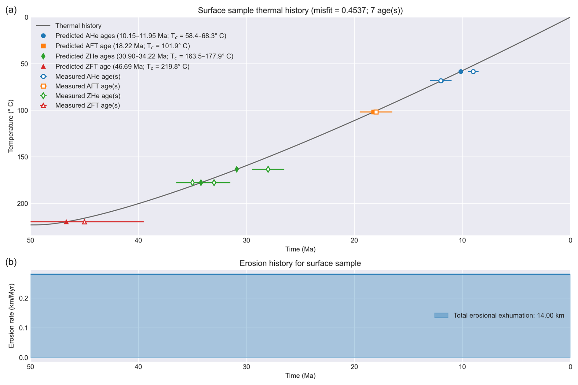
Figure 3 Example thermal history with measured and predicted thermochronometer ages output from T_c1D. (a) Thermal history plot with measured and predicted thermochronometer ages. Predicted ages (filled symbols) plot along the thermal history at their effective closure temperatures, while measured ages (open symbols with horizontal error bars) are located based on their age and predicted effective closure temperature for the corresponding predicted age. The calculated total misfit is shown in the plot title, but the four depositional ages are not displayed. (b) Erosion rate history for the thermal history in (a).

In addition to the age prediction model, there are several variables in T_c1D that affect age prediction. The equivalent spherical radius can be specified for AHe and ZHe age prediction, or will default to an equivalent spherical radius of 60 µm. Uranium and thorium concentrations can also be defined for AHe and ZHe ages, or will default to concentrations of 10 and 40 ppm for uranium and thorium in apatite or 100 and 40 ppm for uranium and thorium in zircon. In addition, it is possible to define a time duration that a tracked particle resides at the initial model temperature prior to the start of a T_c1D thermal simulation. This can be useful for including the effects of radiation damage accumulation without requiring transient temperature calculations during that interval.

The predicted thermochronometer ages can be compared to measured ages in two different ways in T_c1D. First, it is possible to read age data from a data file. In this case, the user must input at least the data type (e.g., AHe), the measured age, and its standard deviation. The user can optionally include a sample ID and depositional age for dated sedimentary samples. If non-zero depositional ages are provided, T_c1D will calculate predicted ages for a tracking particle reaching the surface the time of deposition in the model, assuming zero transport time from the source area. For (U–Th)$/$He ages it is also possible to input an effective uranium (eU) concentration and grain radius. When provided, the sample grain radius and eU values will be used for age prediction, otherwise the default U, Th, and radius values given above will be used. The second option for providing measured ages is to provide one or more measured ages and standard deviations to T_c1D using function parameters or command-line flags. In this case, however, the sample-specific grain radius and/or eU values are not utilized for (U–Th)$/$He age prediction and it is not possible to specify depositional ages. In either case, it is possible to output a summary csv-formatted text file containing the measured and predicted ages and relevant other values such as the eU concentration and grain radius.

A quantitative measure of goodness-of-fit between measured and predicted thermochronometer ages in T_c1D can be calculated using a misfit function (e.g., Fig. 3). By default, the misfit Φ uses the L2 norm between the measured and predicted ages divided by the square root of the summed measured age uncertainties and normalized to the number of samples (e.g., Eq. (8) of Braun et al., 2012),

$$\begin{array}{}\text{(4)}& \mathrm{\Phi }={\displaystyle \frac{\mathrm{1}}{N}}\sqrt{\sum _{i=\mathrm{1}}^N{\displaystyle \frac{{\left(O_i-C_i\right)}^{\mathrm{2}}}{{\mathit{\sigma }}_i^{\mathrm{2}}}}},\end{array}$$

where N is the number of ages, O_i is the ith measured (or observed) age, C_i is the ith predicted (or calculated) age, and σ_i is the standard deviation (uncertainty) for the ith measured age. This default goodness-of-fit approach will produce misfit values that are less than or equal to 1 when the predicted ages fall within the measurement uncertainties on average and greater than 1 otherwise. Another misfit function option is described below for use with inverse models in T_c1D.

3.3 Batch and inverse modeling

In addition to individual forward models, groups of models can be run in T_c1D to either explore parameter sensitivity or invert data to determine ranges of model parameters that best reproduce the measured ages. Both options are briefly described in the sections below.

3.3.1 Sensitivity analysis via batch modeling

The sensitivity of T_c1D models to different model parameters can be assessed using its batch mode. Batch mode is activated by passing a list as a parameter for one or more batch model parameters, by listing multiple values after one or more batch model command-line flags, or by setting the batch mode parameter to be true. A complete list of batch model parameters is available online at the T_c1D documentation site (Whipp, 2025). Batch mode uses the ParameterGrid function from the scikit-learn library (Pedregosa et al., 2011) to generate a list of all permutations of the batch parameters, and T_c1D then runs forward models using each permutation. In contrast to normal forward models that display plots and model results on the screen, however, model input and output values are written to a csv-formatted log file. In this way, parameter sensitivity can easily be assessed and key model outputs, such as predicted ages, can be compared to refine parameter values for individual forward models.

3.3.2 Inverse modeling

Data-driven exploration of thermal and erosional processes can be performed using the inverse mode in T_c1D. The inverse mode in T_c1D searches within ranges of designated model parameters to determine which provide the best fit to a set of measured ages, as well as statistical bounds on the best-fitting parameter ranges. Data inversion takes a Bayesian approach using either the Neighborhood Algorithm (e.g., Sambridge, 1999b, a) or an affine invariant Markov chain Monte Carlo sampler (Goodman and Weare, 2010; Foreman-Mackey et al., 2013). In both cases, the misfit between measured and predicted ages is used to guide the inverse parameter search toward values that provide a better fit to the measured age data. To facilitate inversion, T_c1D defaults to using the χ² equation for calculating a model misfit Φ for inverse models,

$$\begin{array}{}\text{(5)}& \mathrm{\Phi }=\sum _{i=\mathrm{1}}^N{\displaystyle \frac{(O_i-C_i{)}^{\mathrm{2}}}{{\mathit{\sigma }}_i^{\mathrm{2}}}}.\end{array}$$

The χ² equation is used because this simpler misfit function does not depend on the number of measured ages and can more easily be linked to the likelihood function used in both inversion approaches. Each inverse approach is briefly described below.

The Neighborhood Algorithm (Sambridge, 1999b, a) is an inverse modeling algorithm that utilizes the Voronoi diagram to find the nearest neighbor regions under a certain distance norm. The Voronoi diagram is constructed by dividing the parameter space domain into cells, each centered on a data point and containing all points closer to that point than to any other. The misfit value of the point is assigned to the corresponding Voronoi cell. During each iteration of the model, the input values are selected from cells where data misfit is low, allowing the algorithm to reduce the difference between the model prediction and the observed values. Unlike probabilistic methods like Markov Chain Monte Carlo, the Neighborhood Algorithm automatically adapts the search to regions of lower misfit and thus is more computationally efficient. However, the Neighborhood Algorithm is sensitive to local minima of the parameter space, especially for inverse problems involving many parameters to invert. The hyperparameters of the algorithm are available via command-line arguments or the YAML input file, defining the number of iterations, number of initial samples, samples per iteration and number of resampled cells.

In addition to the Neighborhood Algorithm, T_c1D includes an inverse modeling option based on a Markov chain Monte Carlo (MCMC) approach. The current implementation uses the affine invariant ensemble sampler of Goodman and Weare (2010), as implemented in the Python library emcee (Foreman-Mackey et al., 2013). This approach is well suited to inverse problems in which model parameters may be correlated, as the sampler is less sensitive to parameter scaling than conventional single-chain Metropolis methods. Compared to the Neighborhood Algorithm, the MCMC approach provides a more statistically rigorous characterization of posterior parameter distributions and is generally less sensitive to local minima in the misfit landscape, although at a higher computational cost.

In the MCMC workflow, users define the model parameters to be inverted by specifying allowable parameter ranges via command-line arguments or in the input file. These parameter bounds define the search space explored by the sampler. An ensemble of walkers is initialized within the prescribed bounds, and each proposed parameter set is evaluated by running a forward T_c1D model and comparing the predicted thermochronometer ages with the observed data using the inverse-model misfit function described above. Key MCMC hyperparameters, such as the number of walkers, chain length, burn-in period, and thinning interval, can be defined by the user in the input file or via command-line arguments, allowing flexible control over the sampling strategy and computational cost.

The prior distribution is currently defined using uniform bounds on the inverted parameters, together with additional physical constraints where needed to reject non-physical models. For instance, parameter combinations that would imply unrealistic cumulative exhumation or invalid model geometries are excluded from the sampled parameter space.

Assuming independent Gaussian uncertainties on the observed thermochronometer ages, the likelihood function is derived from the misfit function Φ and is evaluated as

$$\begin{array}{}\text{(6)}& \log \mathcal{L}=-{\displaystyle \frac{\mathrm{\Phi }}{\mathrm{2}}},\end{array}$$

where Φ corresponds to the χ² misfit between observed and predicted ages.

The posterior probability is then evaluated from the combination of these prior constraints and the likelihood function. For each accepted model evaluation, T_c1D stores the sampled parameter values and the associated posterior probability values. After discarding an initial burn-in period and optionally thinning the chains, the retained samples can be used to characterize posterior parameter distributions and parameter trade-offs.

To facilitate interpretation of inversion results, T_c1D can produce parameter chains, pairwise parameter scatter plots, and corner plots showing the marginal and joint posterior distributions of the inverted parameters. These diagnostics allow users to evaluate the convergence of the Markov chains and visualize parameter correlations.

While the Neighborhood Algorithm is efficient for rapid exploration of parameter space, the MCMC approach provides a more comprehensive assessment of parameter uncertainties and trade-offs, making the two methods complementary in practice. The MCMC implementation can be run in serial mode or in parallel using MPI, which is advantageous since each likelihood evaluation requires a forward thermo-kinematic model calculation. This makes the MCMC option particularly useful for estimating parameter uncertainty and for assessing the range of model solutions that are compatible with a given thermochronologic dataset.

4 What can T_c1D do?

Here we present a few examples of the types of simulations that can be peformed using T_c1D. This is not meant to be an exhaustive list, but rather demonstrate some case studies that are amenable to exploration using T_c1D and may be more difficult to simulate in other thermal history or thermo-kinematic modeling software packages.

4.1 Example 1: Exhumation of an emplaced pluton

This first example considers a pluton that is emplaced in the crust at the start of the numerical experiment, then undergoes conductive cooling and later crustal exhumation (similar to, for example, Nguyen et al. (2022) or Cooper et al., 2026). The pluton is emplaced with a temperature of 1000 °C and a thickness of 2 km between 8–10 km depth at 30 Ma and held at that temperature for 1 Myr. The effects of the latent heat of crystallization are not included. No erosion is applied (advection velocity equals zero) during 30–10 Ma and then 9 km of exhumation is imposed at a constant rate of 0.9 km Myr⁻¹ from 10–0 Ma, displacing the Moho from its initial depth of 44 km to a final depth of 35 km. Default values are used for all other model parameters.

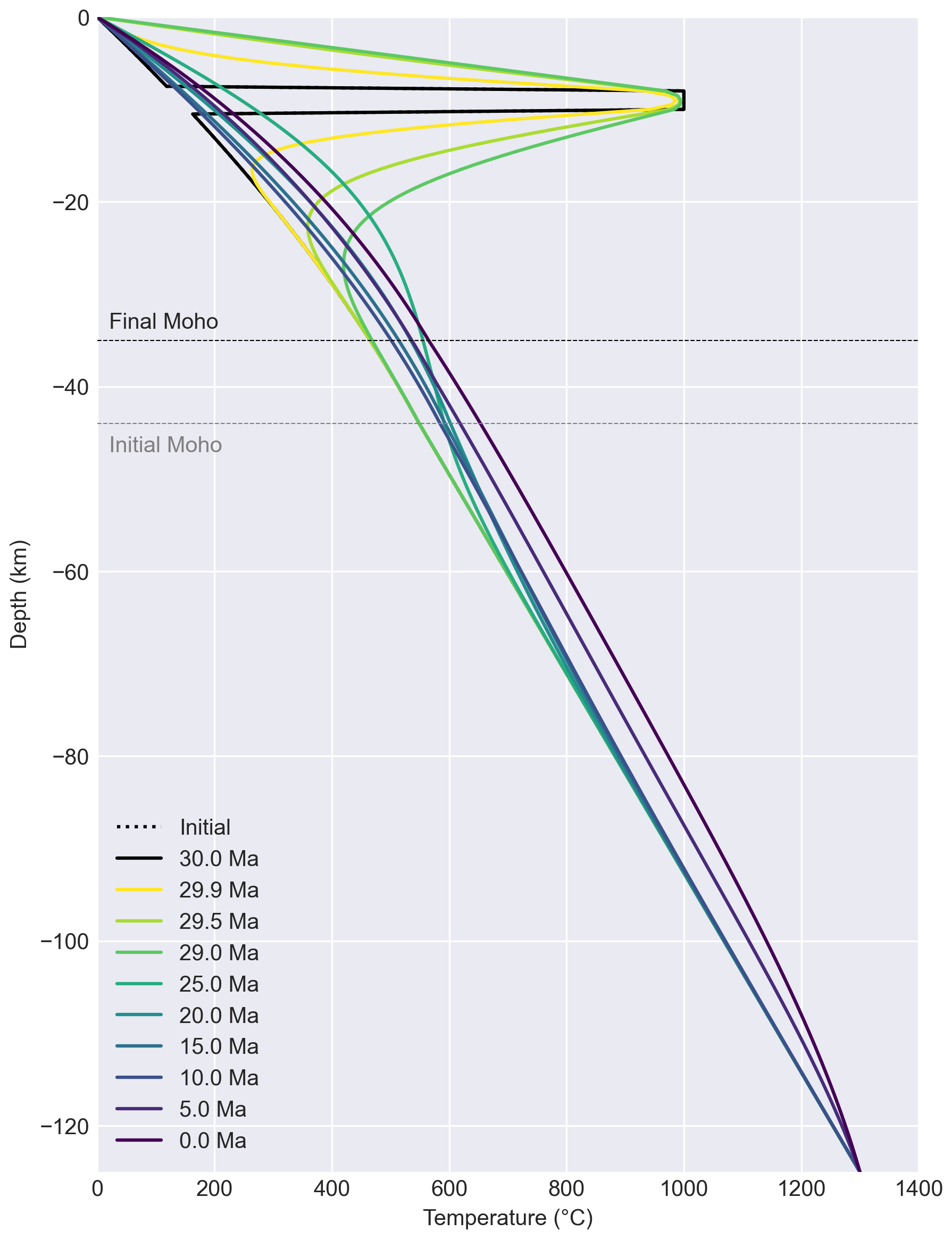
Figure 4 Lithospheric geotherms at various times during a 30 million year T_c1D numerical experiment that starts with an initial stage of pluton intrusion. The 2 km-thick pluton is held at a constant temperature of 1000 °C from 30–29 Ma at depths of 8–10 km, followed by conductive cooling from 29–10 Ma. From 10–0 Ma, the entire lithosphere is exhumed at a rate of 0.9 km Myr⁻¹. This results in exhumation of the Moho from an initial depth of 44 km to a final depth of 35 km.

The thermal effects of magmatism on upper crustal temperatures are clear in this example, but only the ZFT thermochronometer records cooling directly related to magmatism. The thermal distrubance caused by the pluton increases temperatures by more than 800 °C at the emplacement depths of 8–10 km when active and by a smaller amount in the crust above and below the pluton for several million years afterward (Fig. 4). By 25 Ma, however, this thermal effect has diminished considerably, leaving temperatures at most ∼150 °C higher than their conductive steady state across the entire crust (e.g., geotherms at 25–10 Ma in Fig. 4). The final phase of exhumation from 10–0 Ma increases temperatures across the entire lithosphere as heat is advected to shallower depths in the model (e.g., geotherms at 5–0 Ma in Fig. 4). The combination of pluton-related heating and later exhumation produces a thermal history in which the tracked particle within the pluton is initially heated to 1000 °C, cools rapidly to ∼200 °C from ∼29–24 Ma, and then undergoes a final phase of gradual cooling during exhumation from 10–0 Ma (Fig. 5). This cooling history results in a ZFT age of ∼24 Ma, roughly 5 Myr younger than the cessation of plutonic activity, and AHe, AFT, and ZHe ages of ∼7–3 Ma, corresponding to the later exhumation phase (Fig. 5). This example illustrates the sensitivity of low-temperature thermochronometers to processes such as crustal magmatism, but also the challenge of interpreting age data due to the combination of long timescales for conductive cooling and interactions of magmatism and crustal exhumation that can produce ages that vary considerably among the different chronometers.

Figure 5 Thermal history, predicted thermochronometer ages, and exhumation history for the pluton emplacement example. (a) The cooling history (dark gray line) shows rapid cooling after pluton activity ceases followed by a period of slow cooling prior to moderate cooling during exhumation from 10–0 Ma. Predicted thermochronometer ages (colored markers) generally correspond to the late stage of exhumation, except the older ZFT age that records post-magmatic cooling. (b) The exhumation history shows no activity from 30–10 Ma followed by exhumation at a constant rate of 0.9 km Myr⁻¹ from 10–0 Ma.

4.2 Example 2: Age evolution during exhumation

As a second example, we consider the evolution of thermochronometer ages during exhumation of a thrust sheet over 50 Myr. In this case, erosion type 4 is used in T_c1D, which involves instantaneous emplacement of a thrust sheet of a specified thickness atop the existing crust (e.g., Oxburgh and Turcotte, 1974; Davy and Gillet, 1986) and its subsequent erosion. Thermally, this model duplicates temperatures from the upper section of the model crust equal to the thrust sheet thickness and “stacks” those temperatures atop the existing crust. After stacking, the temperatures re-equilibrate during exhumation of part or all of the thrust sheet. For this example, a 10 km-thick thrust sheet is emplaced at 30 Ma and 15 km of rock (the thrust sheet plus five kilometers of the footwall) are eroded during 30–0 Ma. In this example, however, ages are predicted for tracked particles reaching the model surface every 1 Myr, showing how the various chronometers are reset during exhumation and how ages vary between the hanging wall and footwall of the thrust system. Default values are used for all other model parameters and additional plots showing the evolution of geotherms and the thermal history for this model can be found at the link under the heading Code and data availability.

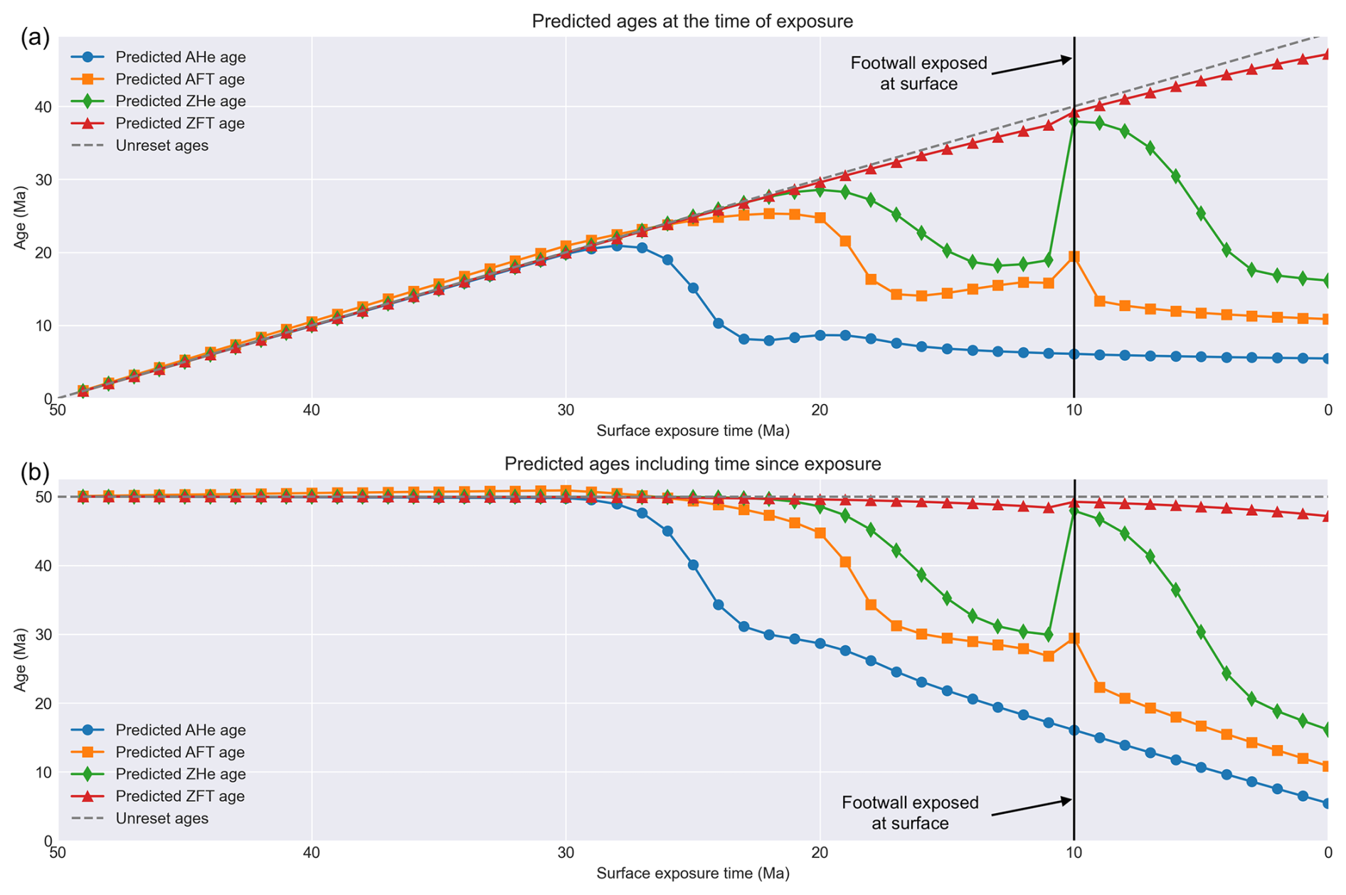
Figure 6 Evolution of predicted thermochronometer ages during exhumation of a thrust sheet from 30 Ma to present. Predicted ages are shown for the apatite and zircon (U–Th)$/$He and fission-track chronometers (AHe, AFT, ZHe, ZFT) with (a) the age at the time the sample reached the model surface during the numerical experiment and (b) the age including time since exposure at the surface (i.e., the age plus the model runtime since exposure). The age evolution presented in (b) is comparable to the ages that would be measured from the accumulation of deposited sediments in a foreland basin, for example. The black vertical lines indicate the time at which exhumation exposes the footwall at the surface (10 Ma). A reference line (dashed dark-gray line) shows the expected age for unreset ages (50 Ma in panel b).

The evolution of predicted ages follows the expected pattern of resetting of the lower temperature chronometers (AHe, AFT) prior to the higher temperature systems (ZHe), but also a jump in ages for some systems as the thrust sheet is fully eroded and footwall rocks are exposed via erosion. Prior to 30 Ma, no exhumation occurs and the predicted ages are all unreset (Fig. 6). As early as ∼27 Ma, partially reset AHe ages begin to appear, as indicated by a deviation from the unreset reference line, and by ∼23 Ma the AHe ages are fully reset and less than 10 Ma when exposed at the model surface (e.g., Fig. 6a). As exhumation continues, partially reset AFT ages appear by ∼20 Ma, followed shortly afterwards by partially reset ZHe ages at ∼18 Ma. Fully reset AFT and ZHe ages are exposed consistently by 17 and 14 Ma, respectively. At 10 Ma, however, ages suddenly increase for the AFT and ZHe systems as the footwall is exhumed and rocks that have not been hot enough to be fully reset are exposed. For ZHe, these ages correspond to unreset ages at 10 Ma and gradually young during exhumation, as seen earlier during exhumation of the thrust sheet (Fig. 6). A similar trend is observed for the AFT ages, but only partially reset ages appear at 10 Ma, and subsequent ages are fully reset. No jump in age is seen for the AHe system, as the 10 km-thick thrust sheet fully resets ages in the footwall after its emplacement. Finally, no reset ZFT ages are observed, reflecting insufficient exhumation depths to expose reset ages. A notable result from this example is that the jump in age during exhumation only occurs for some systems and depends on the thickness of the emplaced thrust sheet. Preservation of such age signals in foreland basin sediments, for example, could provide a means to constrain the timing and thickness of thrust sheet emplacement and exhumation in convergent tectonic settings.

4.3 Example 3: Multi-stage exhumation histories and age data comparison

Here we consider an example of a geological history that involves several stages of exhumation and burial in a cratonic setting over a long duration (>1 Gyr). The model includes 10 stages of erosion or burial and uses an exhumation history defined in the input file for T_c1D rather than using command-line flags. This flexible approach to describing the exhumation history can be used to explore more complex geological and exhumation histories than the general erosion models in T_c1D. This example is based on the exhumation history of the Slave Craton in Canada as described in Ault et al. (2009) and Ault et al. (2015). A summary of the exhumation history for this example and related geological constraints can be found in Table 1.

Ault et al. (2009)Ault et al. (2015)Ault et al. (2015)Ault et al. (2015)Ault et al. (2015)Ault et al. (2015)Ault et al. (2015)Ault et al. (2015)Ault et al. (2015)

Table 1 Exhumation and burial history defined in T_c1D with associated geological constraints.

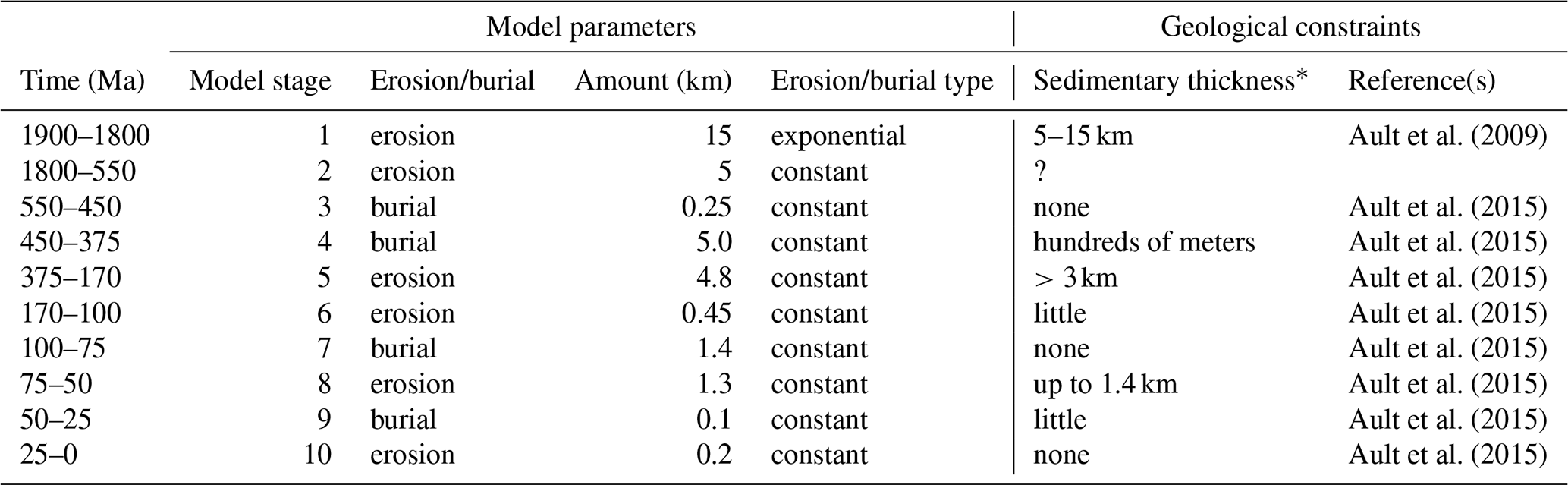
^* Sedimentary thicknesses are listed at the start of each interval.

The thermal history for this example (Fig. 7) supports the proposal by Ault et al. (2015) that Ordovician to Devonian (450–375 Ma) burial is essential for resetting the AHe ages in their dataset, yet using T_c1D we also find a minimum magnitude of burial of at least 5 km is required to achieve the age reset. The early exhumation phase following the last significant tectonic activity (1900–1800 Ma) provides the largest magnitude of cooling and produces ZFT and ZHe ages that are >1800 Ma (Fig. 7). Subsequent gradual exhumation and cooling brings the tracked particle to the surface at 550 Ma, based on geological constraints (Table 1, Ault et al., 2015). Phases of burial from 550–375 Ma increase the temperature of the tracked particle to ∼100 °C before exhumation and cooling from 375–100 Ma bring the tracked particle back to the surface. Exhumation during these stages produces respective AFT and AHe of ∼330 Ma and ∼240–290 Ma, consistent with the age range for the measured AHe ages of 337–188 Ma. In this example, the magnitude of burial from 450–375 Ma is 5 km, which is sufficient to reset both the AFT and AHe ages. However, reducing the burial magnitude to 4.5 km produces only partially reset AFT and AHe ages that are ∼725 and ∼1350–275 Ma, respectively (plot can be found in the supplementary plots linked under the heading Code and data availability). Thus, although Ault et al. (2015) states that the magnitude of Ordovician to Devonian burial is >3 km, this can be refined using T_c1D to be ≥5 km. Further exploration of the timing and magnitudes of burial and exhumation using T_c1D in inverse mode (see Sect. 3.3.2 for an example) could further refine the proposed geological history of this cratonic region.

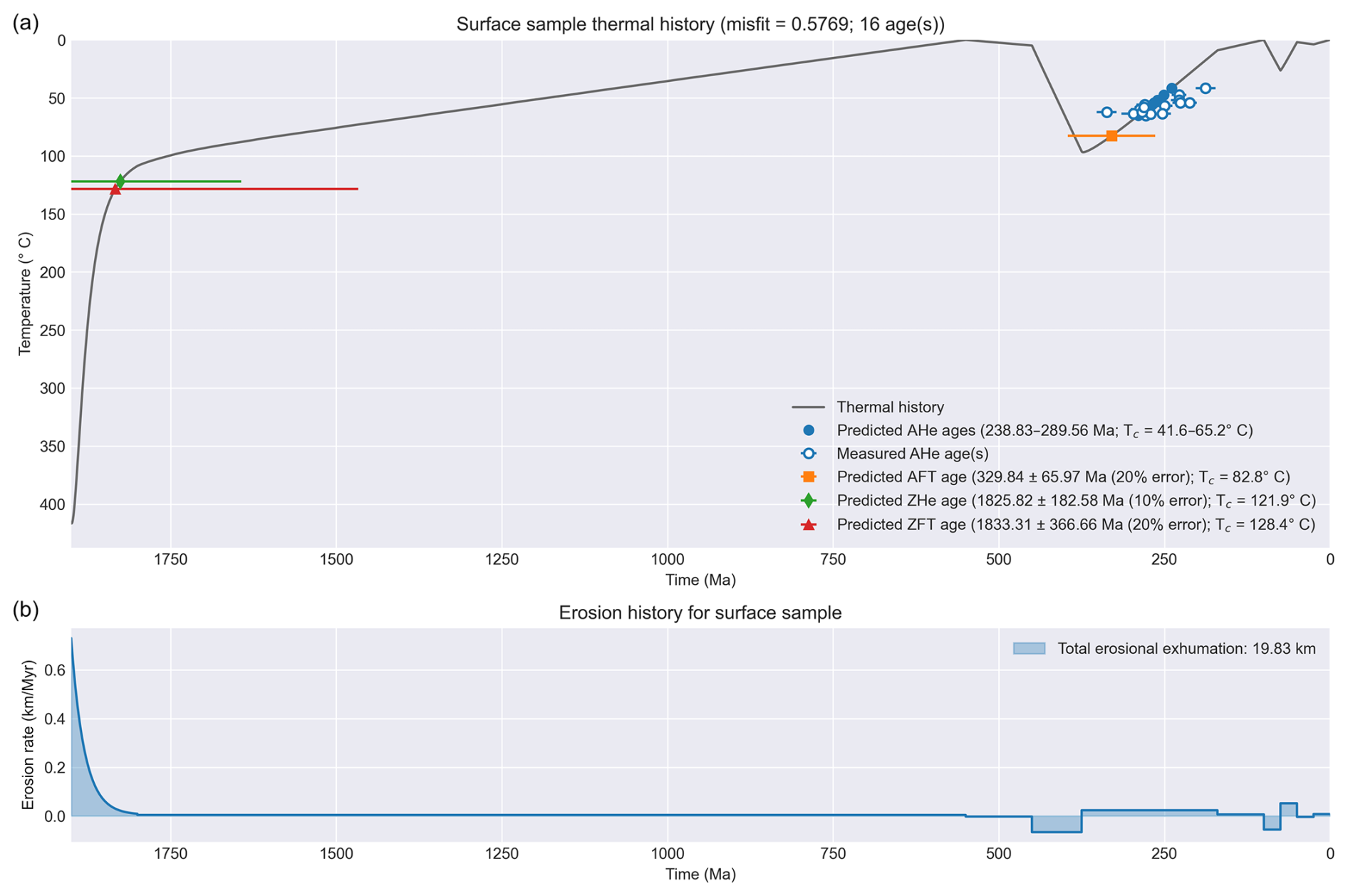
Figure 7 Thermal history, predicted thermochronometer ages, and exhumation history for Slave Craton, Canada. (a) The cooling history (dark gray line) shows initial rapid cooling followed by protracted slow cooling and several reheating and cooling events. Burial and re-heating from 450–375 Ma heats the tracking particle to temperatures sufficient to reset the apatite (U–Th)$/$He and fission-track thermochronometers (blue and orange symbols). Measured apatite (U–Th)$/$He ages (blue symbols with white fill) are quite similar to the predicted ages for this example, as reflected by the low model misfit (<1). Note that the misfit calculated here uses Eq. (4), the default for forward models in T_c1D. Measured age data from Ault et al. (2009). (b) Burial and exhumation history corresponding to the thermal history in (a).

4.4 Example 4: MCMC inversion of a natural thermochronological dataset

To illustrate the Markov chain Monte Carlo (MCMC) inverse modeling functionality in T_c1D, we selected sample 18PE28 from the Marcapata transect in southern Peru from Falkowski et al. (2023) (Fig. 8). This sample provides a useful natural example since it includes four thermochronometric systems that can be directly explored with T_c1D: AHe, AFT, ZHe, and ZFT. Sample 18PE28 is a Permian–Triassic granite collected at 2416 m elevation and yields young to intermediate cooling ages of 1.3±0.4 Ma (AHe), 3.3±0.3 Ma (AFT), 5.5±0.5 Ma (ZHe), and 16.7±1.4 Ma (ZFT), offering relatively strong constraints on late-stage cooling and exhumation history.

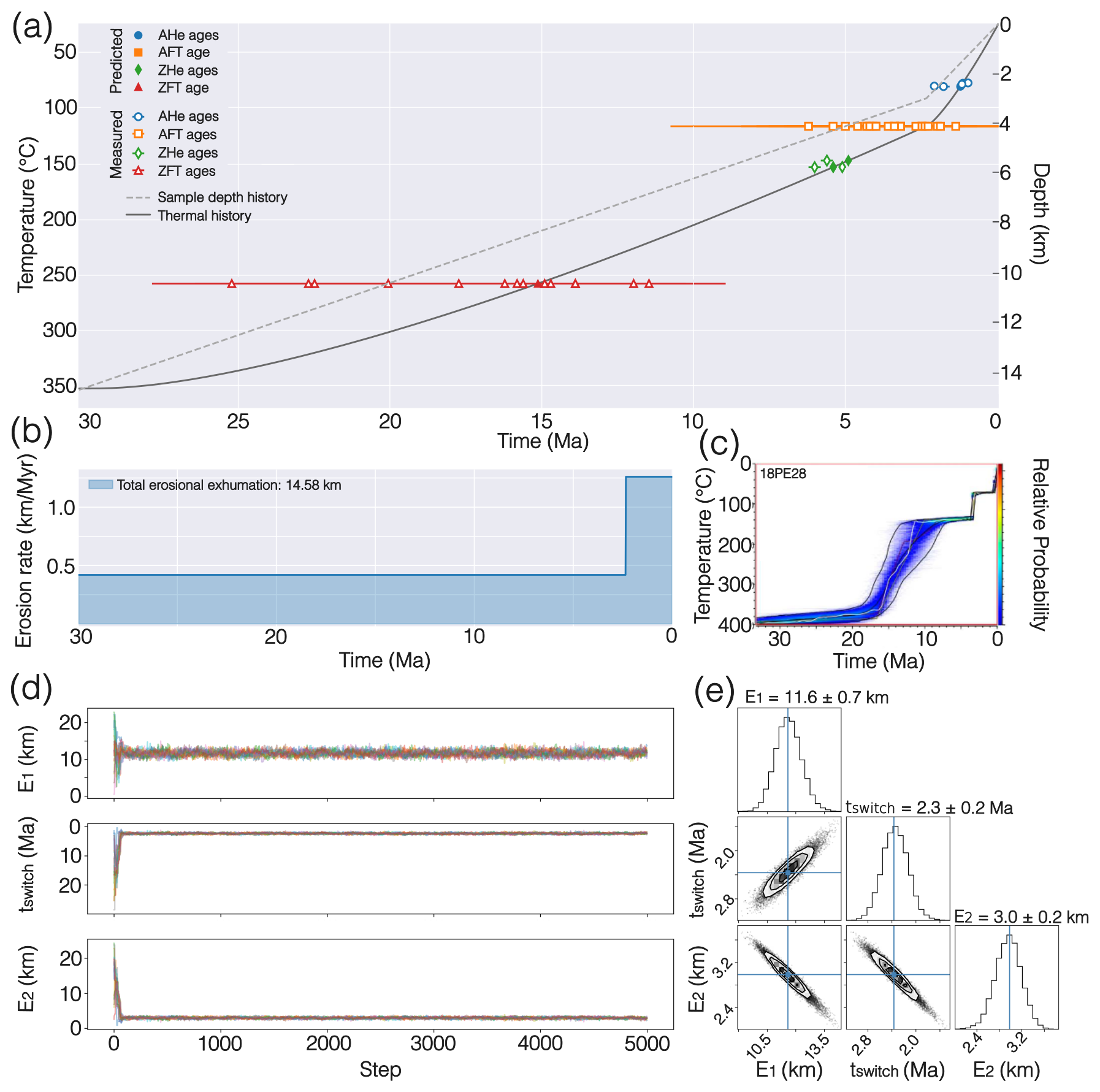
Figure 8 MCMC inversion of sample 18PE28 from Falkowski et al. (2023). (a) Best-fitting forward model showing the surface sample thermal and depth history together with predicted and measured thermochronometer ages for the AHe, AFT, ZHe, and ZFT systems. (b) Inferred erosion history expressed as time-dependent erosion rates derived from the inverted parameters (E₁, t_switch, E₂). (c) Time-temperature paths from QTQt reported by Falkowski et al. (2023), shown for comparison with the Tc1D results. (d) MCMC chains for the three inverted parameters, illustrating convergence and exploration of parameter space. (e) Corner plot showing the marginal posterior distributions and pairwise correlations between parameters, highlighting parameter uncertainties and trade-offs.

The aim of this example is not to reproduce exactly the inverse time-temperature histories presented by Falkowski et al. (2023), but rather to demonstrate how T_c1D can be used to invert a natural multi-system thermochronological dataset using an explicit thermo-kinematic parameterization. In contrast to inverse approaches that primarily return time-temperature paths, T_c1D links the observed ages to a prescribed thermal structure and parameterized erosion history. This allows the inversion results to be interpreted directly in terms of geologically meaningful model parameters, such as the timing and magnitude of changes in erosion rate.

For this illustrative example, we inverted a two-stage erosion history using three free parameters: (1) the total amount of erosion during the first stage ($E_{\mathrm{1}}\in [\mathrm{0.01},\mathrm{25.0}]\mathrm{km}$), (2) the timing of the transition between the two stages ($t_{\text{switch}}\in [\mathrm{0.01},\mathrm{30.0}]\mathrm{Ma}$), and (3) the total amount of erosion during the second stage ($E_{\mathrm{2}}\in [\mathrm{0.01},\mathrm{25.0}]\mathrm{km}$) (Fig. 8). The total model time spans 30 Ma, such that t_switch effectively controls the timing of a potential break in slope in the erosion history. These parameters are internally converted into time-dependent erosion rates (km Myr⁻¹) during forward modeling. The MCMC inversion was performed using 16 walkers and 5000 steps per walker, with the first 500 steps discarded as burn-in and a thinning factor of 3 applied to reduce sample autocorrelation, resulting in a total of 24 000 retained models used for posterior analysis.

The thermal structure and crustal properties were fixed based on representative values for the region following Gérard et al. (2021), including crustal density, heat capacity, thermal conductivity, heat production, surface temperature, and initial Moho depth, while other model parameters were set to commonly used default values.

The inversion recovers a family of solutions that reproduce the observed AHe, AFT, ZHe, and ZFT ages (Fig. 8a), with the best-fitting model providing a close agreement with the measured ages within uncertainty. The corresponding erosion histories (Fig. 8b) consistently indicate an acceleration of erosion around 2 Ma. This timing is in good agreement with the time-temperature paths reported by Falkowski et al. (2023), which show an increase in cooling rates starting at approximately 2 Ma (Fig. 8c). The MCMC diagnostics (Fig. 8d and e) indicate good exploration of parameter space, with well-mixed chains and well-defined posterior distributions for all inverted parameters.

5 Discussion

5.1 What are the best use cases for T_c1D?

The examples presented above demonstrate a range of geological scenarios in which T_c1D can be used to understand how geological processes affect thermochronometer age data. We have also suggested that T_c1D is complementary to available thermal history modeling and more complex thermo-kinematic modeling software, such as Pecube. This raises a natural question: What are the best cases to consider using T_c1D?

Although T_c1D could be used in many cases where it is desirable to explore the effects of varying magnitudes of exhumation, burial, magmatic heating, or the impact of other geological processes, we feel there are four scenarios in which use of T_c1D is most appropriate. First, T_c1D is recommended in cases where the aim is to quantify the magnitudes of burial and/or exhumation, and the primary motion of material is vertical. Such cases could include tectonically inactive regions and regions where the horizontal component of tectonic motion is limited. Because T_c1D does not simulate horizontal motion of rock mass, there may be scenarios where its use could result in misinterpretations of age data due to a large horizontal component of heat transfer, such as in active fold-and-thrust belts. T_c1D could still be used as an exploratory tool in such settings, but it may be more appropriate to consider a more complex thermo-kinematic numerical modeling software package such as Pecube in such situations.

A second scenario where the use of T_c1D is recommended is when working with age data from regions with limited topographic relief or with samples collected across areas with limited relief. The reason for this recommendation is similar to that for the first case: T_c1D uses a 1D heat transfer model and thus may not capture the thermal effects of topography on subsurface isotherms, which could lead to data misinterpretation. Mountain topography typically perturbs the geometry of shallow crustal isotherms (e.g., Stüwe et al., 1994; Mancktelow and Grasemann, 1997), though not always (e.g., Glotzbach et al., 2009), and such an effect is not possible to directly incorporate in T_c1D due to its geometry. As a result, it is possible that modeling thermochronometer data in regions with significant topographic relief could be problematic. Thus, T_c1D may be more safely applied in areas with limited topographic relief, such as areas that are no longer tectonically active or where the topographic effects on crustal isotherms are thought to be minimal. Future versions of T_c1D may include the possibility to correct for the effects of topography on crustal temperatures following the apporach of Ketcham (2025), for example.

A third case where we recommend using T_c1D is for the interpretation of multi-chronometer datasets or groups of samples thought to have experienced similar thermal histories. In this case, the benefit for use of T_c1D mainly relates to the potential to quantify rates of exhumation and/or burial using T_c1D's inverse mode. Having multiple temperature sensitivities from multiple chronometers provides better constraint on the possible thermal histories that could produce the measured age data. The same concept applies to thermal history models like HeFTy, QTQt, or Thermochron.jl, but the strength of T_c1D in this case is the potential to use a data-driven inverse approach to quantify rates of geological processes more directly. This type of inverse modeling could also be done together with thermal history modeling or as a preparatory step in more complex modeling using Pecube.

The final case where using T_c1D is suggested is to simply explore the effects of various geological processes on thermochronometer data. T_c1D provides a tool with which researchers can explore how varying rates and magnitudes of burial and/or exhumation affect predicted ages, as well as the impact of different thermal processes (e.g., magmatism) and rock thermo-physical properties (e.g., radiogenic heat production). Varying different parameter values can illustrate when and by how much different processes impact predicted ages. This can aid not only in data interpretation, but also in planning where to sample, which thermochronometer systems to consider, and other factors that can help ensure the signal sought in collected samples is likely to be present. Similarly, the effects of different geological processes can be introduced to students interactively using T_c1D to help them gain intuition about what matters when studying geological processes using thermochronology.

5.2 Integration with other tools

The thermal histories produced in T_c1D can be exported and read directly into the T_cplotter software (Whipp and Ketcham, 2022) to further explore the combined effects of the geological processes simulated in T_c1D and factors affecting individual mineral grains such as variability in grain size or eU concentration. T_cplotter uses the same FT annealing and He diffusion equations as T_c1D but can calculate variations in cooling ages and effective closure temperatures simultaneously for desired ranges of grain size and eU (and hence variability in radiation damage accumulation) to simulate their effect on He diffusion and resulting calculated AHe and ZHe ages. While grain sizes and eU concentrations can be varied for individual mineral grains in T_c1D, the T_cplotter software produces contour plots for ranges of these values that can be illustrative when considering the possible impact of radiation damage or variation in grain size on predicted thermochronometer ages or effective closure temperatures. The thermal histories produced by T_c1D are stored in plain text files, which can also be readily adapted to be read into other modeling software such as HeFTy.

5.3 Model limitations

In the preceding test we have noted some of the benefits and limitations of T_c1D, and we summarize the main limitations of the T_c1D here. First, T_c1D uses a one-dimensional thermal and kinematic framework in which heat transport and rock movement occur only in the vertical direction. Consequently, the model cannot take into account lateral variations in temperature, topography, or material properties. In particular, processes such as lateral heat transfer due to dipping faults or topography-driven perturbations of isotherms are unable to be simulated, as noted above.

Second, the current version of T_c1D imposes constant temperature boundary conditions at the surface and base of the model that do not vary in time. This is not a limitation of the numerical method, but there is not yet support for time-varying boundary condition temperatures. Similarly, rock thermo-physical properties for the crust and lithosphere are prescribed using simplified layer-based values that also do not generally evolve through time, except when using specific processes implemented in the model, such as magmatic intrusion or lithospheric removal. These restrictions may limit its applicability in settings with long and complex thermal evolutions, such as cratonic regions or orogenic systems with multiple deformation phases.

Third, T_c1D simulates the thermal history of a single vertical column of rock and is therefore best suited to the interpretation of thermochronological data from individual samples or from locations where samples are thought to experience similar burial or exhumation histories. While multiple samples can be analyzed individually, the model does not explicitly account for spatial relationships between them. As a result, it cannot directly represent lateral variations in exhumation history or thermal structure, nor test spatially varying processes such as fault activity and/or lateral exhumation gradients. Similarly, although vertical sampling profiles (e.g., age-elevation relationships) can be explored on a sample-by-sample basis, the model cannot explicitly reproduce the continuous structure of such profiles.

5.4 Ongoing and future developments

Recent major developments in T_c1D have focused on increasing flexibility in defining burial and exhumation histories and extending the capabilities of T_c1D for inverse modeling. These features are currently under active development and testing, and are briefly outlined here to highlight the evolving capabilities of the model.

The first development concerns the introduction of the flexible, multi-stage erosion framework (ero_type=0), in which exhumation or burial histories are defined as a sequence of successive stages. Each stage can be assigned a different erosion style (e.g., constant, linear, or exponential) and corresponding parameterization, allowing complex and more realistic time-dependent histories to be represented within a single model run. The same framework can also be used in inverse mode, where selected stage parameters are treated as free variables within prescribed bounds. This new erosion model type in T_c1D is usable from the T_c1D input file.

A second development is the implementation of a trans-dimensional (i.e., variable-dimension) Markov chain Monte Carlo (Reversible Jump MCMC) approach for inversion of multi-stage erosion histories. In contrast to fixed-dimension inversion methods, this approach allows both the number of erosion stages and the parameters defining the erosion laws of each stage to be inferred simultaneously from the data. The current implementation uses a set of stochastic moves that include parameter perturbations as well as changes in model dimension (i.e., the number of erosion stages), enabling exploration of models with varying levels of complexity within a single inversion workflow. This provides a flexible framework for balancing model fit and model complexity (parsimony) when modeling thermochronological data. A working version of a first implementation of this framework is in the development version of T_c1D, will be available in a future release of the code after further testing and refinement.

In addition to the ongoing code development, there are several planned features in T_c1D that are worth noting. First, we intend to improve support for modeling thermochronometer ages of sedimentary deposity in T_c1D. It is possible at present to include the time of deposition for predicted ages in the T_c1D data file, but the only effect this has in the current implementation is to calculate an age at the surface at the time corresponding to deposition and then add time to that age between when it is deposited and the end of the simulation. We hope to improve this in future versions of T_c1D by allowing subsequent burial and heating to enable users to explore complex thermal histories in foreland basins, for example. Second, we plan to explore implementing a means for incorporating the effects of topography on predicted ages. Although T_c1D uses a 1D thermal model, it is possible to account for the effects of surface topography on crustal temperatures (e.g., Fox et al., 2014; Ketcham, 2025). Thus, we intend to test various options for handling surface topography to enable the use of T_c1D in regions with significant topographic relief or with elevation transects. Finally, a longer term goal is to develop a flexible age prediction library for use with T_c1D that would suport more thermochronometer systems. This is not likely to be implemented in the near future, but is planned as a future development goal to broaden the potential range of chronometers that can be modeled using T_c1D.

6 How to get started using T_c1D

We aim to make it easy to get started using T_c1D and list below two options in order of simplicity:

1. Using Binder. The easiest way to get started using T_c1D is to launch an interactive Jupyter notebook using Binder from https://mybinder.org/v2/gh/HUGG/TC1D/HEAD?urlpath=%2Flab%2Ftree%2Fnotebooks%2Fexplore_tc1d.ipynb (last access: 30 April 2026). This link will open a web application hosted on a temporary cloud server that allows the user to explore use of T_c1D without installing anything. User data files can be uploaded, run T_c1D, and output plots saved in this way. However, this is not recommended for inverse models using T_c1D.

2. Installing the Python package. T_c1D is available as an installable Python package using pip. This involves slightly more work, as the user will need to have access to a working Python environment to run T_c1D locally. The advantage of this option is that files are saved automatically, versus working in Binder which deactivates after ∼10 min of inactivity and does not store data between sessions, and inverse models can be run more easily using the input file or command-line options.