the Creative Commons Attribution 4.0 License.
the Creative Commons Attribution 4.0 License.
 | 06 Apr 2020
Re-evaluating 14C dating accuracy in deep-sea sediment archives
Bryan C. Lougheed
Philippa Ascough
Andrew M. Dolman
Ludvig Löwemark
Brett Metcalfe
The current geochronological state of the art for applying the radiocarbon (14C) method to deep-sea sediment archives lacks key information on sediment bioturbation. Here, we apply a sediment accumulation model that simulates the sedimentation and bioturbation of millions of foraminifera, whereby realistic 14C activities (i.e. from a 14C calibration curve) are assigned to each single foraminifera based on its simulation time step. We find that the normal distribution of 14C age typically used to represent discrete-depth sediment intervals (based on the reported laboratory 14C age and measurement error) is unlikely to be a faithful reflection of the actual 14C age distribution for a specific depth interval. We also find that this deviation from the actual 14C age distribution is greatly amplified during the calibration process. Specifically, we find a systematic underestimation of total geochronological error in many cases (by up to thousands of years), as well as the generation of age–depth artefacts in downcore calibrated median age. Even in the case of “perfect” simulated sediment archive scenarios, whereby sediment accumulation rate (SAR), bioturbation depth, reservoir age and species abundance are all kept constant, the 14C measurement and calibration processes generate temporally dynamic median age–depth artefacts on the order of hundreds of years – whereby even high SAR scenarios (40 and 60 cm kyr−1) are susceptible. Such age–depth artefacts can be especially pronounced during periods corresponding to dynamic changes in the Earth's Δ14C history, when single foraminifera of varying 14C activity can be incorporated into single discrete-depth sediment intervals. For certain lower-SAR scenarios, we find that downcore discrete-depth true median age can systematically fall outside the calibrated age range predicted by the 14C measurement and calibration processes, thus leading to systematically inaccurate age estimations. In short, our findings suggest the possibility of 14C-derived age–depth artefacts in the literature. Furthermore, since such age–depth artefacts are likely to coincide with large-scale changes in global Δ14C, which themselves can coincide with large-scale changes in global climate (such as the last deglaciation), 14C-derived age–depth artefacts may have been previously incorrectly attributed to changes in SAR coinciding with global climate. Our study highlights the need for the development of improved deep-sea sediment 14C calibration techniques that include an a priori representation of bioturbation for multi-specimen samples.
- Article
(4741 KB) - Full-text XML
-
Supplement
(928 KB) - BibTeX
- EndNote


1.1 Background and rationale
For over half a century, radiocarbon (14C) dating has been applied to deep-sea sediment archives. The material that is typically analysed from these archives consists of the calcareous tests of foraminifera. The minimum amount of material required for viable 14C analysis has meant that researchers have had to pick tens to hundreds of individual foraminifera specimens (depending on specimen size) from a single discrete-depth core interval (typically 1 cm of core depth) and combine these into a single sample for analysis. Such multi-specimen samples are likely to be heterogeneous in 14C activity (i.e. combine individual specimens of varying true age). The 14C laboratory measurement (and reported machine error) applied to such an amalgamated multi-specimen sample will simply represent the mean 14C activity of the total carbon of all individual specimens. Consequently, the true intra-sample 14C age heterogeneity of a sample is concealed from the researcher. Failure to consider the actual 14C age heterogeneity of multi-specimen samples can lead to downcore 14C age artefacts when post-depositional processes mix foraminifera with differing 14C activities, which is especially pronounced during periods of dynamic Δ14C. Furthermore, one must also take into consideration that younger specimens within a sample contribute exponentially more to the sample's mean 14C activity than older specimens do, a process referred to as the isotope mass balance effect (Erlenkeuser, 1980; Keigwin and Guilderson, 2009), due to 14C being a radioactive isotope (specimen 14C activity decreases exponentially with the passing of time).
Systematic bioturbation has long been recognised as an inherent feature of deep-sea sediment archives (Bramlette and Bradley, 1942; Arrhenius, 1961; Olausson, 1961). Long-established mathematical models of bioturbation in deep-sea sediment archives consider the uppermost ∼10 cm of a sediment archive to be uniformly mixed due to active bioturbation – the bioturbation depth (BD) (Berger and Heath, 1968; Berger and Johnson, 1978; Berger and Killingley, 1982). The presence of such a BD has been supported by the detection of a uniform mean age in the uppermost intervals of sediment archives (Peng et al., 1979; Trauth et al., 1997; Boudreau, 1998; Teal et al., 2008) and suggested by the 14C analysis of single foraminifera (Lougheed et al., 2018). The total range of single-specimen ages mixed within the BD is dependent upon two main factors: the depth of the BD itself and the sediment accumulation rate (SAR), both of which can exhibit spatio-temporal variation due to environmental and biological factors (Müller and Suess, 1979; Trauth et al., 1997). The presence of uniform mixing within the BD throughout the sedimentation history of a deep-sea sediment archive ultimately results, in the case of temporally constant SAR and BD, in the single-specimen population of discrete sediment intervals being characterised by an exponential probability density function (PDF) for true age, with a maximum probability for younger ages and a long tail towards older ages. The existence of such a distribution has been supported by the post-depositional mixing of tephra layers (Bramlette and Bradley, 1942; Nayudu, 1964; Ruddiman and Glover, 1972; Abbott et al., 2018) and the smoothing out of the downcore mean signal (Guinasso and Schink, 1975; Pisias, 1983; Schiffelbein, 1984; Bard et al., 1987; Löwemark et al., 2008; Trauth, 2013), the smoothing of which can change downcore in tandem with foraminiferal abundance changes (Ruddiman et al., 1980; Peng and Broecker, 1984; Paull et al., 1991; Löwemark et al., 2008). If SAR, BD and the Δ14C history of the planet were all to be temporally constant, then the idealised 14C activity PDF of each discrete depth (expressed as, for example, the 14C∕12C ratio or normalised as fraction modern [F14C]) would, therefore, exhibit the combination of two exponential functions (the exponential PDF of true age plus the exponential PDF of 14C activity vs. time predicted by the half-life of 14C). However, the distribution of the 14C activity PDF is further complicated by the fact that 14C activity vs. time is not always the exact exponential function that would be predicted by the radioactive half-life of 14C, seeing as the Earth's carbon reservoirs exhibit a dynamic Δ14C history, as demonstrated by temporal changes in atmospheric 14C activity (Suess, 1955, 1965; de Vries, 1958; Reimer et al., 2013). These changes are brought about by changes in 14C production in the atmosphere in combination with climatic and oceanic influence upon the carbon cycle (Craig, 1957; Damon et al., 1978; Siegenthaler et al., 1980). Furthermore, non-uniform mixing of the oceans can contribute to temporal changes in local water 14C activity at a given coring site, further affecting the idealised PDF shape.
When applying the 14C method to sediment core material, researchers represent the 14C activity of a discrete-depth interval using a normal (Gaussian) distribution, based on the conventional mean 14C age (a reporting convention for 14C activity) and measurement error reported by the 14C laboratory (Stuiver and Polach, 1977). In some cases, this 14C age normal distribution is widened by researchers to also incorporate a reservoir age uncertainty, but it remains a normal distribution. This normal distribution of 14C age is subsequently calibrated using a suitable reference record of past Δ14C (e.g. those produced by the IntCal group), allowing researchers to arrive at an estimation of the discrete-depth interval's true (i.e. calendar) age. Such an approach inherently excludes the effects of bioturbation, because one would not expect a normal 14C age distribution to be representative of a discrete-depth interval for the reasons described in the previous paragraph. Currently, systematic investigation is lacking into whether neglecting to include the effects of bioturbation has significant impact upon the interpretative accuracy of 14C dating as it is currently applied in palaeoceanography, i.e. if it may ultimately lead to spurious geochronological interpretations.
1.2 Experimental design
Here, we take advantage of computer modelling to construct an ideal experimental design whereby we can evaluate how the current 14C state of the art within palaeoceanography would work in the case of best-case sediment conditions. Such best-case conditions do not exist in the field, meaning that a computer modelling environment can uniquely be used to create such a best-case scenario, which is ideal for testing the current state of the art. We use the Δ14C-enabled, single-specimen SEdiment AccuMUlation Simulator (SEAMUS) (Lougheed, 2020). This model uses the long-established understanding of bioturbation as included in existing bioturbation models (Trauth, 2013; Dolman and Laepple, 2018), but it differs in that it explicitly simulates the accumulation and bioturbation of single foraminifera, each with individually assigned 14C activities, to create a synthetic sediment archive history. Subsequently, current palaeoceanographic subsampling and 14C dating practices are virtually applied to the 1 cm discrete-depth sediment intervals of the model's outputted synthetic archive, resulting in discrete-depth 14C ages and calibrated ages that are representative of the existing palaeoceanographic state of the art. These results are subsequently compared to the actual discrete-depth true age distributions within the model, allowing us to quantitatively evaluate contemporary palaeoceanographic 14C measurement and calibration techniques. By keeping multiple model input parameters constant, we can construct an experimental environment whereby we have full control over the degrees of freedom. This modelling approach allows us to test, at a most fundamental level, the accuracy of the current 14C dating state of the art as applied to deep-sea sediments.
2.1 The synthetic core simulation
The SEAMUS model (Lougheed, 2020) synthesises n single foraminifera raining down from the water column per simulation time step, whereby n is the capacity of the synthetic sediment archive being simulated (analogous to sediment core radius) scaled to the SAR of the time step as predicted by an inputted age–depth relationship (Lougheed, 2020). To provide good statistics, all simulations use a time step of 5 years and 104 synthetic foraminifera per centimetre of core depth. An abundance of 104 specimens per centimetre is also similar to a best-case scenario value for a particular sample in the field (Broecker et al., 1992).
In each time step, all newly created single foraminifera are assigned an age (corresponding to the time step), a sediment depth (according to the age–depth input), and a 14C age (in 14C BP) and normalised 14C activity (in F14C) based on Marine13 (Reimer et al., 2013) after the application of a prescribed reservoir age for the time step. For older sections of the Marine13 calibration curve, where only 10-year time steps are available, linear interpolation is used to provide a 5-year 14C activity time step resolution. Within SEAMUS, all single foraminifera older than the oldest available age within the chosen calibration curve (in this case Marine13) are assigned the same 14C activity: that of the analytical blank, which must be set in the simulation. In this way, the model incorporates the principles of 14C dating, whereby individual very old foraminifera contained within a sample will contribute a 14C signal equivalent to the analytical blank. Here, we choose to set the simulation's analytical blank value to 46 806 14C BP (more precisely the F14C equivalent thereof), which corresponds to the lowest activity level in the Marine13 calibration curve. The analytical blank activity in most laboratories is somewhat lower (e.g. >50 000 14C BP), but we have no way of accurately applying an activity to single foraminifera older than the oldest value contained within Marine13. Rather than infer a Δ14C history beyond the limit of Marine13, we simply set the analytical blank in our simulation to 46 806 14C BP. In some scenarios we wish to investigate parameters within an experimental construct with temporally constant Δ14C, and in such scenarios we assign 14C activity (as F14C) as follows: , where t is the single foraminifera age in years before 1950 CE, and R(t) is the reservoir age for age t.
After the creation of all new single foraminifera within the synthetic core for a specific time step, bioturbation is simulated. Specifically, for each time step the depth values corresponding to all simulated foraminifera within the contemporaneous BD are each assigned a new depth by way of uniform random sampling of the BD interval. In this way, uniform mixing of foraminifera within the BD is simulated by following the established understanding of bioturbation (Berger and Heath, 1968; Trauth, 2013). All of the aforementioned processes are repeated for every simulation time step until such point that the end of the age–depth input (i.e. the final core top) is reached. All simulations are initiated at 70 ka (in true age) in order to confidently exclude the influence of model spin-up effects upon our period of interest (0–45 ka), given the possibility of a given centimetre of sediment to have a long tail of older foraminifera specimens. While SEAMUS can in principle be run on a local machine, to save time multiple simulations were run in parallel on a computing cluster provided by the Swedish National Infrastructure for Computing (SNIC) at the Uppsala Multidisciplinary Center for Advanced Computational Science (UPPMAX).
2.2 Virtual discrete-depth analysis
After the completion of the synthetic core simulation, synthetic foraminifera (and corresponding values for true age, F14C and 14C age) are picked from each discrete 1 cm interval of the sediment core. In this study, we assume best-case scenarios where it is possible to pick all whole foraminifera contained within the sediment intervals. Subsequently, each of these picked 1 cm samples also undergoes a synthetic 14C determination analogous to a perfect accelerator mass spectrometry (AMS) measurement, whereby it is assumed that the AMS determination perfectly reproduces the mean 14C activity (in F14C) of the sample. Within the discrete-depth subsampling simulation, this mean 14C activity is calculated by taking the mean of all F14C values of all the single foraminifera contained within the picked sample. As mentioned in Sect. 2.1, the analytical blank is already included when assigning 14C to single foraminifera, meaning that the influence of the analytical blank upon sample AMS measurements is incorporated.
Using the Libby half-life, a sample's mean F14C value is also reported as a conventional 14C age determination (in 14C yr). All such synthetic determinations are assigned a synthetic 1σ measurement error analogous to a best-case scenario laboratory counting error for a large sample. The prescribed synthetic measurement error ranges from 30 14C yr in the case of near-modern samples to 500 14C yr in the case of samples nearing the blank value. Specifically, when assigning measurement errors to synthetic AMS determinations, a 14C determination of 1.0 F14C is assumed to have a measurement error of 30 14C yr, and a determination with the F14C value (i.e. one 14C yr younger than the blank value) is assumed to have a measurement error of 500 14C yr. Errors (in 14C yr) for intermediate dates are linearly interpolated to F14C.
The synthetic laboratory 14C determinations and associated measurement uncertainties for each 1 cm discrete-depth sample are subsequently converted to calibrated years within SEAMUS using the embedded MatCal (v 2.6) 14C calibration software (Lougheed and Obrochta, 2016), the Marine13 calibration curve (Reimer et al., 2013) and a prescribed reservoir age (according to the scenario – see following sections) to produce a calibrated age probability density function (PDF) and 95.4 % highest posterior density (HPD) credible interval(s) for every centimetre core depth, i.e. analogous to what would be typically produced using contemporary palaeoceanography methods in the case of every discrete centimetre of core depth being exhaustively 14C dated. The MatCal software calibrates ages in F14C space, resulting in an accurate calibration, especially in the case of older samples or samples with large uncertainty.
In order to investigate the baseline accuracy when applying 14C dating to deep-sea sediment cores, the first simulations in this study consider a number of best-case scenarios. Essentially, we seek to test how well the current application of 14C within palaeoceanography would function in the case of such a best-case scenario, thus testing the current state of the art at a most fundamental level. In such simulations, we assume that Marine13 constitutes a perfect reconstruction of past surface-water 14C activity at the synthetic core site, and we therefore employ a temporally constant reservoir age (ΔR=0 14C yr). Furthermore, we assume a scenario involving synthetic sediment cores with temporally constant SAR and BD, and we also assume that the synthetic core is made up of a single planktonic foraminiferal species with a temporally constant abundance (104 cm−1) and specimen size. A total of five best-case scenarios are carried out, with five different SAR scenarios (5, 10, 20, 40 and 60 cm kyr−1). The BD is set to 10 cm in all cases, following established understanding of global BD (Trauth et al., 1997; Boudreau, 1998). In this scenario, we also assume perfection in subsampling, i.e. the possibility to exhaustively sample all foraminifera material from each 1 cm discrete-depth interval when picking for multi-specimen samples, thus excluding noise due to small sample sizes. The results of these five scenarios are visualised in Figs. 1 and S1–S5 in the Supplement.

Figure 1Overview of results of simulations using Marine13 Δ14C involving multiple constant SAR scenarios (5, 10, 20, 40 and 60 cm kyr−1) with constant BD of 10 cm, constant species abundance of 100 % and 0 % broken foraminifera. All discrete-depth results are plotted against their true median age on the x axes. (a) The discrete-depth offset between mean AMS (i.e. laboratory) conventional 14C age and the idealised mean 14C age. (b) The discrete-depth offset between the true median age and the calibrated median age (i.e. that derived from the 14C measurement and calibration process). (c) The discrete-depth difference between the calibrated highest posterior density (HPD) 95.4 % age range (i.e. that derived from the 14C measurement and calibration process) and the true 95.4 % age range of the sediment. (d, e, f, g, h, i) A visualisation of 14C calibration skill for select discrete-depth samples from various scenarios indicated on the figure panels. The blue histograms represent the actual single-foraminifera simulation output: on the x axis the true age distribution of the single foraminifera (with the blue diamond corresponding to the median true age) and on the y axis the corresponding true 14C age distribution of the single foraminifera (with the blue diamond corresponding to the mean 14C age of all individual foraminifera). All histograms are shown using 30-year or 30 14C yr bin widths. The pink distributions represent the current state of the art in 14C dating. The pink normal distribution on the y axis represents an AMS 14C determination carried out on the single specimens, where the pink square corresponds to its mean. The pink probability distribution on the x axis represents the calibrated age PDF arising from the calibration of the aforementioned AMS 14C determination using Marine13 (Reimer et al., 2013) and MatCal (Lougheed and Obrochta, 2016), where the pink square represents the median calibrated age. Also shown, for reference, are the Marine13 calibration curve 1σ (dark grey) and 2σ (light grey) confidence intervals.
A second set of best-case scenarios takes into account that relatively older foraminifera contained within a given discrete depth of core sediment will have accumulated a longer residence time in the active bioturbation depth. Due to their longer residence time in the active bioturbation depth, these foraminifera are more likely to be broken and/or partially dissolved (Rubin and Suess, 1955; Ericson et al., 1956; Emiliani and Milliman, 1966; Barker et al., 2007), and they are thus less likely to be picked by palaeoceanographers, who preferentially pick whole, unbroken foraminifera specimens for analysis. In this way, palaeoceanographers exclude the oldest, least well preserved fraction of the sediment. An indication of the BD residence time of single specimens for a given 1 cm discrete depth is shown in Fig. 2 for all five simulated SAR scenarios, along with the median and 90th percentile residence time. The percentage of broken specimens within the sediment archive is chiefly governed by the aforementioned BD residence time, bottom water chemistry (Bramlette, 1961; Berger, 1970; Parker and Berger, 1971), and the susceptibility of a particular foraminifera species to dissolution or breakage (Ruddiman and Heezen, 1967; Boltovskoy, 1991; Boltovskoy and Totah, 1992). Previous studies have indicated that the percentage of foraminifera exhibiting test breakage for typically analysed species at locations above the lysocline can hover around 10 % (Le and Shackleton, 1992). In the second set of best-case scenarios we, therefore, exclude from the picking process for each 1 cm discrete depth all foraminifera with a number of bioturbation cycles greater than the 90th percentile for that particular discrete depth. This broken foraminifera percentage of 10 % is applied to all five SAR scenarios (5, 10, 20, 40 and 60 cm kyr−1) in a second set of best-case scenarios (shown in Figs. 3 and S6–S10). One should be aware, however, that BD residence time likely varies with SAR itself: when sediment accumulation is slower, single specimens remain in the BD for relatively longer than in the case of faster SAR (Bramlette, 1961).
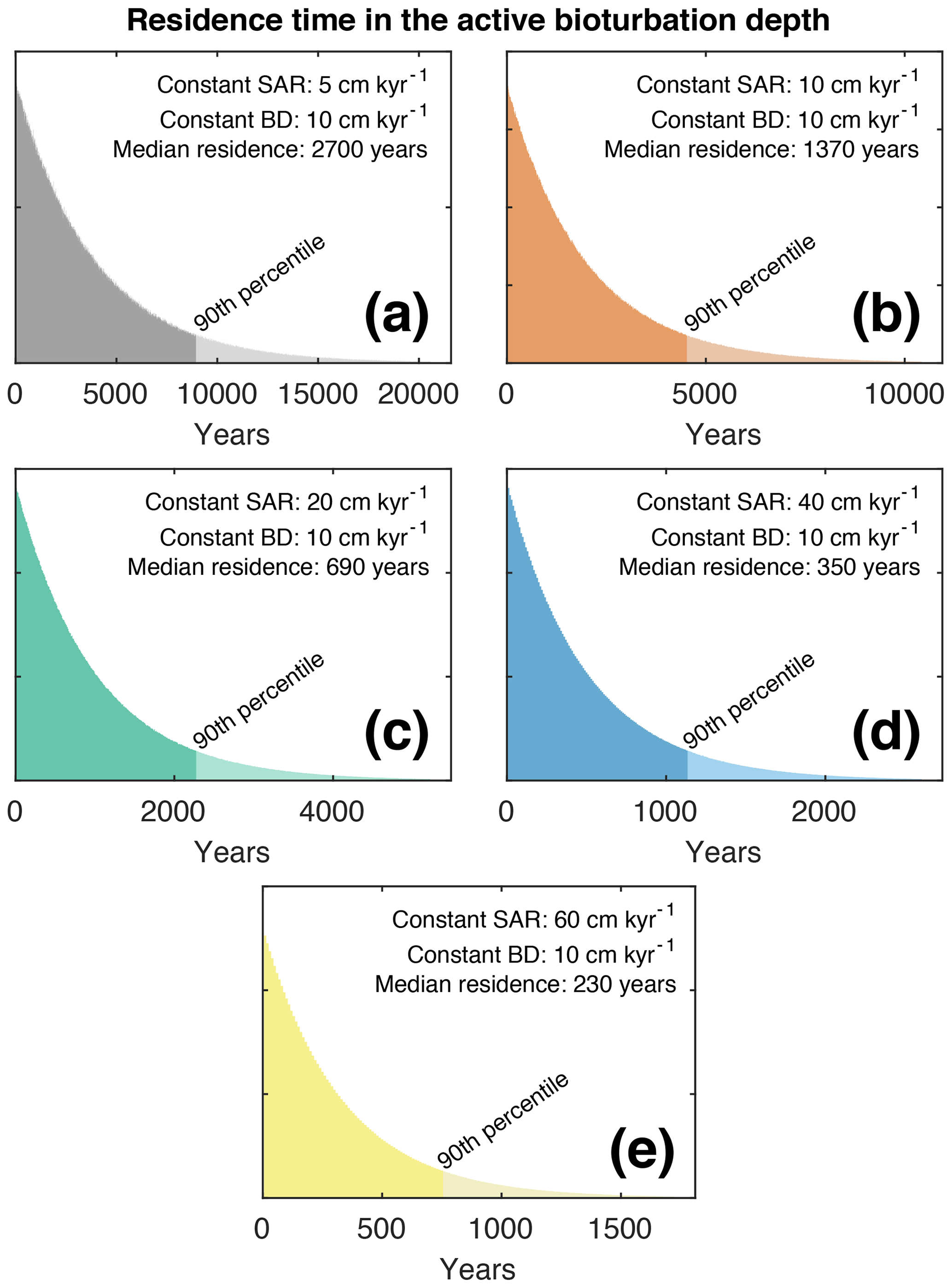
Figure 2An overview of residence time of single foraminifera within the active BD for the various simulation scenarios detailed in Fig. 1, i.e. with a constant BD of 10 cm and a SAR of (a) 5, (b) 10, (c) 20, (d) 40 and (e) 60 cm kyr−1.
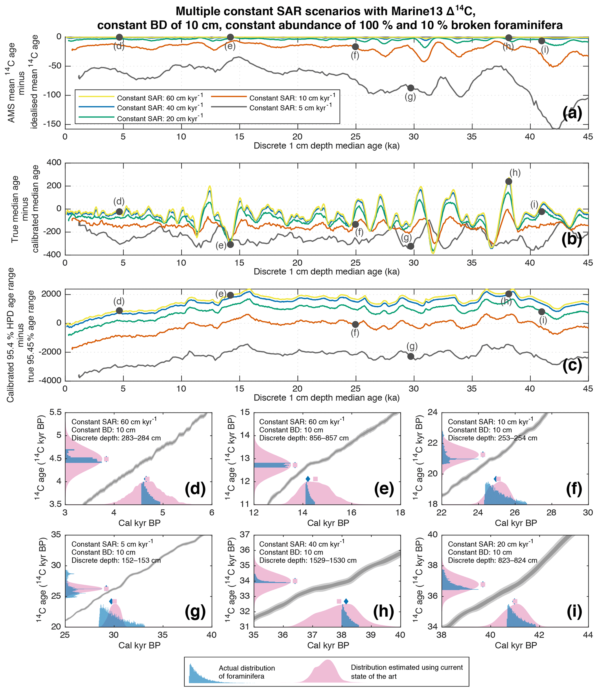
Figure 3Overview of results of simulations using Marine13 Δ14C involving multiple constant SAR scenarios (5, 10, 20, 40 and 60 cm kyr−1) with constant BD of 10 cm, constant species abundance of 100 % and 10 % broken foraminifera. All discrete-depth results are plotted against their true median age on the x axes. (a) The discrete-depth offset between mean AMS (i.e. laboratory) conventional 14C age and the idealised mean 14C age. (b) The discrete-depth offset between the true median age and the calibrated median age (i.e. that derived from the 14C measurement and calibration process). (c) The discrete-depth difference between the calibrated highest posterior density (HPD) 95.4 % age range (i.e. that derived from the 14C measurement and calibration process) and the true 95.4 % age range of the sediment. (d, e, f, g, h, i) A visualisation of 14C calibration skill for select discrete-depth samples from various scenarios indicated on the figure panels. The blue histograms represent the actual single-foraminifera simulation output: on the x axis the true age distribution of the single foraminifera (with the blue diamond corresponding to the median true age) and on the y axis the corresponding true 14C age distribution of the single foraminifera (with the blue diamond corresponding to the mean 14C age of all individual foraminifera). All histograms are shown using 30-year or 30 14C yr bin widths. The pink distributions represent the current state of the art in 14C dating. The pink normal distribution on the y axis represents an AMS 14C determination carried out on the single specimens, where the pink square corresponds to its mean. The pink probability distribution on the x axis represents the calibrated age PDF arising from the calibration of the aforementioned AMS 14C determination using Marine13 (Reimer et al., 2013) and MatCal (Lougheed and Obrochta, 2016), where the pink square represents the median calibrated age. Also shown, for reference, are the Marine13 calibration curve 1σ (dark grey) and 2σ (light grey) confidence intervals.
3.1 14C age artefacts
Radiocarbon analysis focuses on determining the mean 14C activity of a particular sample, which is reported together with an associated analytical error. This mean activity of samples is often considered in the literature as conventional 14C age in 14C BP. Conventional 14C age, a unit of convenience, is linear vs. time, whereas 14C activity is actually exponential vs. time, due to 14C being a radioactive isotope. Therefore, with increasing age heterogeneity of a sample, we can expect an increased offset between the AMS conventional 14C age of a sample (the mean measured activity of the homogenised sample reported as conventional age) and the idealised mean of the conventional 14C ages of all single foraminifera within the sample. In Fig. 1, we compare the simulated AMS mean conventional 14C age calculated for each discrete depth to the idealised mean 14C age (based on the mean value of all single foraminifera conventional 14C ages contained within a sample). The resulting offset can help shed light upon how the measurement of age-heterogenous material is inherently biased towards younger (higher 14C activity) specimens contained within the sample. We find that the AMS mean 14C age is generally younger than the idealised mean 14C age in all cases. This effect can be attributed to the fact that younger foraminifera within a heterogeneous sample contribute exponentially more to a sample's mean 14C activity (what the measurement process is actually analysing) than older foraminifera do. This bias towards younger foraminifera is most apparent in cases with large intra-sample heterogeneity, such as in scenarios with lower SAR (Fig. 1a), and it is also reduced somewhat in the case of more broken foraminifera (Fig. 3a), due to lesser older foraminifera being picked, thus reducing the age heterogeneity. In the case of the highest SAR scenarios (>40 cm kyr−1) the aforementioned bias is insignificant in a practical sense in that it falls within the typical 14C measurement error. For all scenarios, superimposed upon the general bias are artefacts of the Earth's dynamic Δ14C history, caused by foraminifera from times of markedly differing Δ14C to be mixed together into a single sample, thus altering a sample's 14C activity distribution and causing downcore dynamic offsets between AMS mean 14C age and idealised mean 14C age. The most pronounced example of these artefacts can be seen during known periods of dynamic Δ14C, such as during the Laschamp geomagnetic event (ca. 40–41 ka) (Guillou et al., 2004; Laj et al., 2014), when a large spike in atmospheric 14C production occurred (Muscheler et al., 2014). We note that our simulations assign single foraminifera 14C activity using the Marine13 calibration curve, while newer records of Δ14C (Cheng et al., 2018) suggest that the Laschamp Δ14C excursion may have been of greater magnitude than was previously thought. A larger excursion would generate even more pronounced 14C artefacts in the downcore, multi-specimen, discrete-depth record. Furthermore, there may exist as yet undiscovered short-lived excursions in Δ14C (Miyake et al., 2012, 2017; Mekhaldi et al., 2015).
We can also visualise how well a sample's 14C activity probability distribution function (PDF) is represented by a distribution based on its mean AMS-measured 14C activity and 1σ measurement error. This visualisation is shown on the vertical axes of Figs. 1d–i and 2d–i for a number of simulated discrete depths for the different SAR scenarios with a BD of 10 cm. It can be clearly seen that the normal distribution derived from a sample's AMS mean measurement and associated uncertainty is a poor representation of a sample's actual 14C activity distribution.
3.2 Calibration amplifies 14C age distribution mischaracterisation
When estimating a true age distribution for a particular sample, researchers calibrate a normal distribution of 14C age using suitable calibration curve (in this case Marine13). As discussed in the previous section, the aforementioned normal distribution of 14C activity derived from the measurement mean and machine error is not a faithful representation of the actual 14C activity distribution for a particular discrete depth. Such a misrepresentation has the potential to be further amplified during the calibration process itself, potentially resulting in a poor estimation of a discrete depth's 95.4 % age range and/or median age, the latter of which is often used to calculate, for example, sedimentation rates or represents the region of highest probability which will steer age–depth modelling routines. In Fig. 1b (0 % broken foraminifera) and Fig. 3b (10 % broken foraminifera), we show the offset between each discrete depth's true median age, and the corresponding median age derived from the 14C calibration process. We find large offsets for all constant SAR scenarios, ranging from ∼200 years in the case of the 60 cm kyr−1 scenario up to ∼700 years in the case of the 5 cm kyr−1 scenario. In certain low-SAR scenarios that coincide with intervals of the calibration curve that are highly resolved (e.g. the late Holocene), the discrete-depth true median age can consistently fall outside the 68.2 % age range predicted by the 14C measurement and calibration processes. A 68.2 % certainty suggests that, statistically, the true median will fall outside of the 68.2 % calibrated age range in only 31.8 % of cases, but, in the case of the 5 cm kyr−1 scenario (Fig. S1), the true median falls outside of the 68.2 % calibrated age range for 84 % of the discrete depths spanning the 5 to 0 ka period. In the case of 10 % broken foraminifera, this effect is reduced.
All offsets for all scenarios vary dynamically downcore, meaning that they can potentially cause spurious interpretations of changes in SAR. Furthermore, as these offsets occur during periods of dynamic Δ14C, which can be caused by large-scale changes in the carbon cycle caused by climate shifts (such as during the last deglaciation), it is possible that some apparent changes in SAR in the palaeoceanographic literature may have been erroneously attributed to climate processes, when they may be (partially) an artefact of the current application of 14C measurement and calibration within palaeoceanography.
Using the simulation output, it is also possible to quantitatively estimate how well the current 14C measurement and calibration state of the art applied within palaeoceanography estimates the true age range contained within discrete-depth sediment intervals. The offset between the calibrated 95.4 % age range and the true 95.4 % age range for each discrete depth for all SAR scenarios is shown in Fig. 1c (0 % broken foraminifera) and Fig. 3c (10 % broken foraminifera), and it is further visualised for all scenarios in Figs. S1–S10. For the lower SAR scenarios, the current application of 14C dating within palaeoceanography significantly underestimates the total age range contained within each discrete depth by many thousands of years. The underestimation is less in the case of the scenario with 10 % broken foraminifera. In the case of higher-SAR scenarios, the discrete-depth 95.4 % age range predicted by the 14C calibration process is similar to that of the discrete-depth 95.4 % age range of the sediment itself. In some cases with very high SAR, the 14C calibration process actually overestimates the 95.4 % age range (e.g. Figs. 1e, 3e, S5 and S10).
3.3 The influence of the analytical blank
A general consequence of bioturbation and the subsequent mixing of single foraminifera specimens is that older foraminifera become systematically mixed upwards throughout the sedimentation history of a sediment archive. This general mixing can have a particular consequence near the analytical limit of the 14C method in that foraminifera with a 14C activity that is lower than a laboratory-based analytical sensitivity can become mixed into samples. Samples with a 14C age that is equal to or older than the established 14C blank value (i.e. the samples 14C activity falls below the detection limit of the analytical process) are commonly referred to as “14C-dead”. Within older intervals of heterogeneous deep-sea sediment archives, it is possible that a sample with an apparent measured 14C age younger than the 14C blank value can already contain a significant proportion of 14C-dead foraminifera. The presence of these 14C-dead specimens within a sample will bias the sample's apparent measured 14C age towards a value that is too young, because they will contribute a 14C activity to the sample that is equivalent to the laboratory's analytical blank. Such artefactually young 14C ages could ultimately erroneously be interpreted as age–depth features. In Table 1, the very first downcore occurrence of at least one simulated 14C-dead foraminifer is detailed for each of the aforementioned constant SAR scenarios introduced in Sect. 3. In the case of low-SAR scenarios with 0 % broken foraminifera, 14C-dead foraminifera are already present in discrete-depth samples with apparent AMS ages that would normally be considered well above the 14C blank value, e.g. an apparent AMS age of 22 647 14C BP in the case of 5 cm kyr−1, and 33 747 14C BP in the case of 10 cm kyr−1. However, the contribution of 14C-dead foraminifera at these levels may still be insignificant. The exact percentage contribution of 14C-dead foraminifera to discrete-depth AMS determinations is, therefore, detailed in Fig. 4a, c, e, g and i. From this analysis, it transpires that the first occurrence of at least 1 % contribution of 14C-dead foraminifera to discrete-depth AMS determinations occurs in the case of AMS ages of 39 158 and 43 601 14C BP, respectively, for the 5 and 10 cm kyr−1 scenarios. The percentage increases quickly further downcore. In the case of scenarios involving 10 % broken foraminifera, older foraminifera within discrete-depth sediment intervals are no longer whole, and therefore they are not picked for samples by a palaeoceanographer preferring whole specimens. The consequence of this effect is that the first occurrence of picked 14C-dead whole foraminifera occurs much further downcore (Table 1, Fig. 4b, d, f, h and j). This finding further underlines the importance of understanding foraminifera preservation conditions for particular species and/or water chemistry, and the associated consequences for 14C dating.
Table 1The first downcore discrete-depth where “14C-dead” whole foraminifera occur (i.e. ndead≥1) for the various constant SAR and broken foraminifera scenarios discussed in Sect. 3 of this study. Also shown are the simulated median true ages, AMS 14C ages and median 14C calibrated ages corresponding to the discrete depth. The simulation analytical blank value is set to 46 806 14C BP (see Sect. 2.1), thus any single foraminifera with a 14C age older than that blank value are assumed “14C-dead”.


Figure 4An estimation of the contribution of “14C-dead” (i.e. activity below the analytical blank value) foraminifera to discrete-depth sample activity plotted against the apparent AMS 14C mean age of the discrete-depth sample. Based on the simulation scenarios detailed in Figs. 1 and 3 with a constant BD of 10 cm and (a) SAR of 5 cm kyr−1 and 0 % broken foraminifera, (b) SAR of 5 cm kyr−1 and 10 % broken foraminifera, (c) SAR of 10 cm kyr−1 and 0 % broken foraminifera, (d) SAR of 10 cm kyr−1 and 10 % broken foraminifera, (e) SAR of 20 cm kyr−1 and 0 % broken foraminifera, (f) SAR of 20 cm kyr−1 and 10 % broken foraminifera, (g) SAR of 40 cm kyr−1 and 0 % broken foraminifera, (h) SAR of 40 cm kyr−1 and 10 % broken foraminifera, (i) SAR of 60 cm kyr−1 and 0 % broken foraminifera, and (j) SAR of 60 cm kyr−1 and 10 % broken foraminifera.
As motivated in the methods section, for practical reasons we have set the 14C analytical blank value to 46 806 14C BP within our model simulations. The laboratory blank value in most laboratories is around ∼50 000 14C BP, or even greater, depending on sample size, preparation conditions and measurement capability. For such greater blank values, essentially the same curves as shown in Fig. 4 would apply (i.e. assuming there are no, as of yet undiscovered, large Δ14C excursions around the period of the blank age) but shifted further to the right on the x axis. In other words, researchers interested in interpreting Fig. 4 in the case of an analytical blank of 50 000 14C BP should simply shift the curves to the right such that the 100 % 14C-dead contribution exactly coincides with 50 000 14C BP on the x axis.
The multiple sediment archive scenarios carried out in Sect. 3 all involved best-case input parameters with constant SAR. In Fig. 5, we carry out four scenarios to investigate the influence of stepwise changes in the following four input parameters: (1) SAR, (2) BD, (3) species abundance and (4) reservoir age (ΔR). In each of the four scenarios, one of the aforementioned input parameters is varied at a certain time, while the other three are kept constant (Fig. 5a–d). In this way, the influence of one of the dynamic input parameters can be independently judged. To further ensure the ability to independently judge the dynamic sediment input parameters, in these scenarios we do not employ a dynamic Δ14C history using Marine13 but instead assign 14C activities to foraminifera using a constant Δ14C history (with an added constant 400-year reservoir age). This constant Δ14C history is assigned as detailed in the methods section (Sect. 2.1). For the calibration process, we also constructed a calibration curve with the same aforementioned constant Δ14C (also with an added constant 400-year reservoir age), whereby the confidence interval sizes of Marine13 are copied for incorporating a realistic calibration uncertainty. The scenario with dynamic ΔR (Fig. 5d) is simulated on the foraminifera by additionally subtracting () or adding () to or from the 14C age of simulated foraminifera younger or older, respectively, than 20 ka. During the simulated picking and calibration processes, it is assumed that the researcher is aware of the change in ΔR, and, during calibration, they apply a ΔR of −100 to all discrete depths shallower than 204 cm and a ΔR of +100 to all discrete depths deeper than 204 cm.
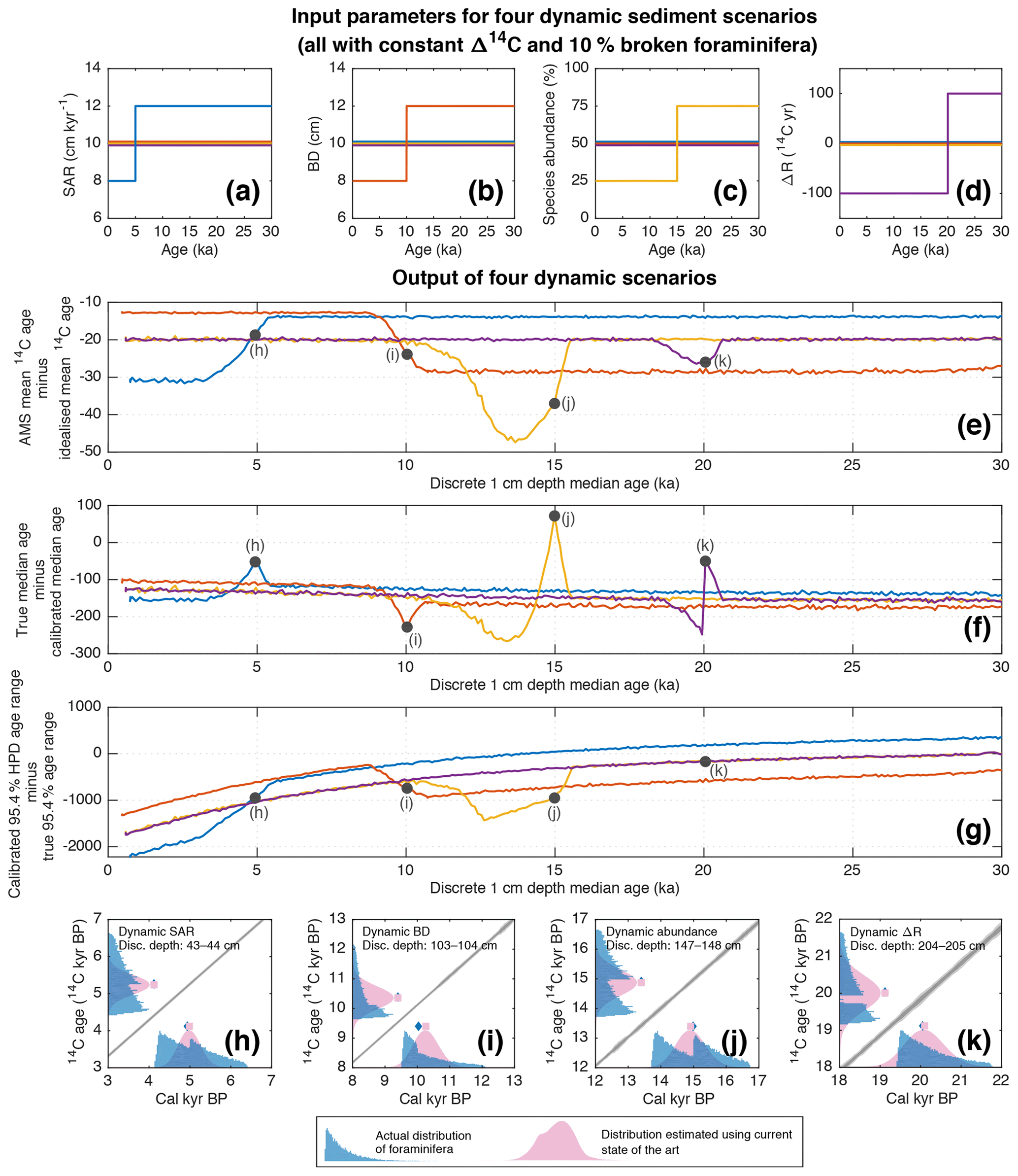
Figure 5Four dynamic input scenarios (each with a unique colour) with constant Δ14C, each involving dynamic input for (a) SAR, (b) BD, (c) species abundance and (d) reservoir age (ΔR). A constant broken foraminifera percentage of 10 % is applied in all cases. (e) For each scenario, the resulting discrete-depth offset between mean AMS (i.e. laboratory) conventional 14C age and the idealised mean 14C age. (f) For each scenario, the discrete-depth offset between the true median age and the calibrated median age (i.e. that derived from the 14C measurement and calibration process). (g) For each scenario, the difference between the calibrated highest posterior density (HPD) 95.4 % age range (i.e. that derived from the 14C measurement and calibration process) and the true 95.4 % age range of the sediment. (h, i, j, k) A visualisation of 14C calibration skill for select discrete-depth samples from various scenarios indicated on the figure panels. The blue histograms represent the actual single-foraminifera simulation output: on the x axis the true age distribution of the single foraminifera (with the blue diamond corresponding to the median true age) and on the y axis the corresponding true 14C age distribution of the single foraminifera (with the blue diamond corresponding to the mean 14C age of all individual foraminifera). All histograms are binned to 30-year or 30 14C yr bin widths. The pink distributions represent the current state of the art in 14C dating. The pink normal distribution on the y axis represents an AMS 14C determination carried out on the single specimens, where the pink square corresponds to its mean. The pink probability distribution on the x axis represents the calibrated age PDF arising from the calibration of the aforementioned AMS 14C determination using a custom-made calibration curve with constant Δ14C (see Sect. 4) and MatCal (Lougheed and Obrochta, 2016), where the pink square represents the median calibrated age. Also shown, for reference, are the calibration curve 1σ (dark grey) and 2σ (light grey) confidence intervals.
The simulations using dynamic parameter inputs demonstrate that temporal changes in any of the four main input parameters (SAR, BD, species abundance, ΔR) can result in the generation of 14C-induced age–depth artefacts in the discrete-depth domain, due to the median calibrated age dynamically deviating from the true median age downcore (Fig. 5f). We also note that the changes in the input parameters can cause the 14C measurement and calibration processes to generate artefacts in the over- or underestimation of the true 95.4 % age range of the sample by the calibration process, artefacts which are superimposed upon a long-term change in the underestimation of the true age range of the sample caused by a long-term change in the confidence intervals in the calibration curve (Fig 5g). Specifically regarding ΔR, the current method for correcting for reservoir age during calibration, which we apply in this simulation, involves subtracting the ΔR from the AMS date just prior to calibration. This method poses a particular challenge for periods near temporal changes in ΔR, where multi-specimen samples will incorporate single foraminifera with varying individual ΔR values. The blanket application of a single ΔR correction to the entire sample fails to adequately represent the ΔR heterogeneity of the foraminifera population.
The influence of the various dynamic parameters upon the 14C measurement and calibration processes, as outlined in Fig. 5, represent further sources of age–depth bias in addition to the large biases caused by dynamic Δ14C history previously outlined in Sect. 3. Furthermore, as has been detailed in previous studies, changes in abundance and bioturbation depth can in themselves also cause additional general age–depth artefacts, no matter what geochronological method is being used (independent of the 14C method) (Bard, 2001; Löwemark and Grootes, 2004; Löwemark et al., 2008; Lougheed, 2020). Such effects can be seen in age–depth artefacts also visible in the true median age for the dynamic BD scenario (Fig. S12) and the dynamic abundance scenario (Fig. S13). Such artefacts occur in addition to the artefacts related to the 14C measurement and calibration processes, as outlined in this study.
Researchers should be aware that periods of long-term climate change can cause many input parameters to change in concert. For example, the last deglaciation in the North Atlantic is known to be characterised by highly dynamic Δ14C (Stuiver et al., 1986; Reimer et al., 2013), dynamic reservoir age (Austin et al., 1995; Waelbroeck et al., 2001; Butzin et al., 2020) and dynamic foraminiferal abundance (Ruddiman and McIntyre, 1981). It is possible that all of these parameters can combine at once to produce very large age–depth artefacts, which could lead to spurious interpretations regarding the relationship between, for example, the last deglaciation and the perceived magnitude of associated SAR change.
This study demonstrates the possibility of the current 14C measurement and calibration method, as it is applied to multi-specimen samples within palaeoceanography, to produce age–depth artefacts, even in the case of best-case sediment archives where SAR, BD, species abundance and reservoir age are all constant. We find that even high-SAR sediment archives (40 and 60 cm kyr−1) are susceptible to the generation of age–depth artefacts during the 14C measurement and calibration processes. Additional age–depth artefacts can be generated in the case of real-world sediment archives where the aforementioned SAR, BD, species abundance and reservoir age processes are inherently dynamic. Researchers should be aware, therefore, of the possible existence of such artefacts when interpreting deep-sea sediment geochronologies developed using 14C methods applied to multi-specimen samples. Key to understanding the possible existence of such artefacts is a good quantification of the possible magnitude of temporal change in both foraminiferal abundance and preservation conditions, as well as awareness of the possibility of changes in local 14C activity due to the influence of dynamic Δ14C and reservoir age. It may also be necessary to revisit existing studies and re-evaluate the magnitude of changes in deep-sea sediment SAR inferred from 14C-based geochronologies, especially close to periods of dynamic Δ14C and/or dynamic foraminiferal abundance. These 14C-specific artefacts should be considered in addition to previously highlighted general age–depth artefacts that can occur in sedimentary records (Bard, 2001; Löwemark and Grootes, 2004; Löwemark et al., 2008; Lougheed, 2020). One should also consider that paired analysis of multi-specimen samples for both 14C and another proxy could lead to a signal offset between the two proxies due to the 14C method, as currently applied within palaeoceanography, being prone to the generation of the types of age artefacts outlined in this study.
We demonstrate that the failure to take into account the effect of bioturbation upon the (14C) age distribution of foraminifera in multi-specimen samples sourced from deep-sea archives can lead to spurious age interpretations, especially during the 14C calibration process. We propose, therefore, that the 14C calibration process for deep-sea sediment archives could be improved in future studies through the development of a new 14C calibration method including bioturbation a priori, seeing that no information regarding bioturbation is included in the current palaeoceanographic state of the art. This new approach would involve constructing a representative distribution for 14C age that includes a priori information regarding the approximate SAR and BD of the sediment archive, while also taking into account some basic information regarding possible temporal changes in species abundance and ΔR. Such a future development would go some way to providing more realistic uncertainties (i.e. 95.4 % age range) to 14C-derived age–depth geochronologies in deep-sea sediment archives.
Finally, we note that increased automation and cost-effectiveness in 14C analysis of ultra-small carbonate samples (Ruff et al., 2010; Lougheed et al., 2012; Wacker et al., 2013a, b) can allow for the parallel measurement of δ18O, δ13O and 14C on a single foraminifer of suitable size (Lougheed et al., 2018), thereby allowing for the extraction of both age and palaeoclimate data from single foraminifera in a manner that is independent of the sediment depth and bioturbation aspects of deep-sea sediment archives.
Model runs generated by SEAMUS for this publication can be downloaded from the Zenodo repository at https://doi.org/10.5281/zenodo.3735134 (Lougheed et al., 2020).
The supplement related to this article is available online at: https://doi.org/10.5194/gchron-2-17-2020-supplement.
BCL carried out the model runs, with scenarios conceived with input from BM. BCL wrote the article with input from the co-authors.
The authors declare that they have no conflict of interest.
The Swedish National Infrastructure for Computing (SNIC) at the Uppsala Multidisciplinary Center for Advanced Computational Science (UPPMAX) provided computing resources. Two anonymous referees and editor Irka Hajdas are thanked for their contribution to the online discussion forum. Their input helped to significantly improve the article.
This work was funded by Swedish Research Council (Vetenskapsrådet – VR) starting grant number 2018-04992 awarded to Bryan C. Lougheed. Brett Metcalfe was supported by a Laboratoire d'excellence (LabEx) of the Institut Pierre Simon Laplace (LabEx L-IPSL), funded by the French Agence Nationale de la Recherche (grant no. ANR-10-LABX-0018). Andrew M. Dolman was supported by the German Federal Ministry of Education and Research (BMBF) as a Research for Sustainability initiative (FONA) through the PalMod project (FKZ: 01LP1509C). Ludvig Löwemark acknowledges support from the Ministry of Science and Technology (06-2116-M-002-021 to Ludvig Löwemark,) and the Featured Areas Research Center Program within the framework of the Higher Education Sprout Project by the Ministry of Education (MOE) of Taiwan.
This paper was edited by Irka Hajdas and reviewed by two anonymous referees.
Abbott, P. M., Griggs, A. J., Bourne, A. J., and Davies, S. M.: Tracing marine cryptotephras in the North Atlantic during the last glacial period: Protocols for identification, characterisation and evaluating depositional controls, Mar. Geol., 401, 81–97, https://doi.org/10.1016/j.margeo.2018.04.008, 2018.
Arrhenius, G.: Geological record on the ocean floor, in: Oceanography, Am. Assoc. Advan. Sci Washington, DC, 129–148, 1961.
Austin, W. E. N., Bard, E., Hunt, J. B., Kroon, D., and Peacock, J. D.: The 14C Age of the Icelandic Vedde Ash: Implications for Younger Dryas Marine Reservoir Age Corrections, Radiocarbon, 37, 53–62, https://doi.org/10.1017/S0033822200014788, 1995.
Bard, E.: Paleoceanographic implications of the difference in deep-sea sediment mixing between large and fine particles, Paleoceanography, 16, 235–239, 2001.
Bard, E., Arnold, M., Duprat, J., Moyes, J., and Duplessy, J. C.: Reconstruction of the last deglaciation: Deconvolved records of δ18O profiles, micropaleontological variations and accelerator mass spectrometric 14C dating, Clim. Dynam., 1, 101–112, 1987.
Barker, S., Broecker, W., Clark, E., and Hajdas, I.: Radiocarbon age offsets of foraminifera resulting from differential dissolution and fragmentation within the sedimentary bioturbated zone, Paleoceanography, 22, PA2205, https://doi.org/10.1029/2006PA001354, 2007.
Berger, W. H.: Planktonic foraminifera: selective solution and the lysocline, Mar. Geol., 8, 111–138, 1970.
Berger, W. H. and Heath, G. R.: Vertical mixing in pelagic sediments, J. Marine Res., 26, 134–143, 1968.
Berger, W. H. and Johnson, R. F.: On the thickness and the 14C age of the mixed layer in deep-sea carbonates, Earth Planet. Sc. Lett., 41, 223–227, 1978.
Berger, W. H. and Killingley, J. S.: Box cores from the equatorial Pacific: 14C sedimentation rates and benthic mixing, Mar. Geol., 45, 93–125, https://doi.org/10.1016/0025-3227(82)90182-7, 1982.
Boltovskoy, E.: On the destruction of foraminiferal tests (laboratory experiments), Révue de Micropaléontologie, 34, 12–25, 1991.
Boltovskoy, E. and Totah, V.: Preservation index and preservation potential of some foraminiferal species, J. Foramin. Res., 22, 267–273, https://doi.org/10.2113/gsjfr.22.3.267, 1992.
Boudreau, B. P.: Mean mixed depth of sediments: The wherefore and the why, Limnol. Oceanogr., 43, 524–526, https://doi.org/10.4319/lo.1998.43.3.0524, 1998.
Bramlette, M. and Bradley, W.: Geology and biology of North Atlantic deep-sea cores. Part 1. Lithology and geologic interpretations, Prof. Pap. U.S. Geol. Surv., 196 A, 1–34, 1942.
Bramlette, M. N.: Pelagic sediments, in: Oceanography: Invited lectures presented at the International Oceanographic Congress held in New York, 31 August–12 September 1959, edited by: Sears, M., Am. Assoc. Advan. Sci Washington, DC, 67, 345–366, https://doi.org/10.5962/bhl.title.34806, 1961.
Broecker, W., Bond, G., Klas, M., Clark, E., and McManus, J.: Origin of the northern Atlantic's Heinrich events, Clim. Dynam., 6, 265–273, https://doi.org/10.1007/BF00193540, 1992.
Butzin, M., Heaton, T. J., Köhler, P., and Lohmann, G.: A short note on marine reservoir age simulations used in IntCal20, Radiocarbon, https://doi.org/10.1017/RDC.2020.9, online first, 2020.
Cheng, H., Edwards, R. L., Southon, J., Matsumoto, K., Feinberg, J. M., Sinha, A., Zhou, W., Li, H., Li, X., Xu, Y., Chen, S., Tan, M., Wang, Q., Wang, Y., and Ning, Y.: Atmospheric 14C∕12C changes during the last glacial period from Hulu Cave, Science, 362, 1293–1297, https://doi.org/10.1029/2006PA001354, 2018.
Craig, H.: The Natural Distribution of Radiocarbon and the Exchange Time of Carbon Dioxide Between Atmosphere and Sea, Tellus, 9, 1–17, https://doi.org/10.1111/j.2153-3490.1957.tb01848.x, 1957.
Damon, P. E., Lerman, J. C., and Long, A.: Temporal Fluctuations of Atmospheric 14C: Causal Factors and Implications, Annu. Rev. Earth Pl. Sc., 6, 457–494, https://doi.org/10.1146/annurev.ea.06.050178.002325, 1978.
de Vries, H.: Variation in concentration of radiocarbon with time and location on Earth, Proceedings of the Koninklijke Nederlandse Akademie van Wetenschappen B, 61, 94–108, 1958.
Dolman, A. M. and Laepple, T.: Sedproxy: a forward model for sediment-archived climate proxies, Clim. Past, 14, 1851–1868, https://doi.org/10.5194/cp-14-1851-2018, 2018.
Emiliani, C. and Milliman, J. D.: Deep-sea sediments and their geological record, Earth-Sci. Rev., 1, 105–132, https://doi.org/10.1016/0012-8252(66)90002-X, 1966.
Ericson, D. B., Broecker, W. S., Kulp, J. L., and Wollin, G.: Late-Pleistocene Climates and Deep-Sea Sediments, Science, 124, 385–389, https://doi.org/10.1126/science.124.3218.385, 1956.
Erlenkeuser, H.: 14C age and vertical mixing of deep-sea sediments, Earth Planet. Sc. Lett., 47, 319–326, https://doi.org/10.1016/0012-821X(80)90018-7, 1980.
Guillou, H., Singer, B. S., Laj, C., Kissel, C., Scaillet, S., and Jicha, B. R.: On the age of the Laschamp geomagnetic excursion, Earth Planet. Sc. Lett., 227, 331–343, https://doi.org/10.1016/j.epsl.2004.09.018, 2004.
Guinasso, N. L. and Schink, D. R.: Quantitative estimates of biological mixing rates in abyssal sediments, J. Geophys. Res., 80, 3032–3043, https://doi.org/10.1029/JC080i021p03032, 1975.
Keigwin, L. D. and Guilderson, T. P.: Bioturbation artifacts in zero-age sediments, Paleoceanography, 24, PA4212, https://doi.org/10.1029/2008PA001727, 2009.
Laj, C., Guillou, H., and Kissel, C.: Dynamics of the earth magnetic field in the 10–75 kyr period comprising the Laschamp and Mono Lake excursions: New results from the French Chaîne des Puys in a global perspective, Earth Planet. Sc. Lett., 387, 184–197, https://doi.org/10.1016/j.epsl.2013.11.031, 2014.
Le, J. and Shackleton, N. J.: Carbonate Dissolution Fluctuations in the Western Equatorial Pacific During the Late Quaternary, Paleoceanography, 7, 21–42, https://doi.org/10.1029/91PA02854, 1992.
Lougheed, B. C.: SEAMUS (v1.20): a Δ14C-enabled, single-specimen sediment accumulation simulator, Geosci. Model Dev., 13, 155–168, https://doi.org/10.5194/gmd-13-155-2020, 2020.
Lougheed, B. C. and Obrochta, S. P.: MatCal: Open Source Bayesian 14C Age Calibration in Matlab, Journal of Open Research Software, 4, e42, https://doi.org/10.5334/jors.130, 2016.
Lougheed, B. C., Snowball, I., Moros, M., Kabel, K., Muscheler, R., Virtasalo, J. J., and Wacker, L.: Using an independent geochronology based on palaeomagnetic secular variation (PSV) and atmospheric Pb deposition to date Baltic Sea sediments and infer 14C reservoir age, Quaternary Sci. Rev., 42, 43–58, 2012.
Lougheed, B. C., Metcalfe, B., Ninnemann, U. S., and Wacker, L.: Moving beyond the age–depth model paradigm in deep-sea palaeoclimate archives: dual radiocarbon and stable isotope analysis on single foraminifera, Clim. Past, 14, 515–526, https://doi.org/10.5194/cp-14-515-2018, 2018.
Lougheed, B. C., Ascough, P., Dolman, A. M., Löwemark, L., and Metcalfe, B.: Model runs generated by publication “Re-evaluating 14C dating accuracy in deep-sea sediment archives” [Data set], Zenodo, https://doi.org/10.5281/zenodo.3735135, 2020.
Löwemark, L. and Grootes, P. M.: Large age differences between planktic foraminifers caused by abundance variations and Zoophycos bioturbation., Paleoceanography, 19, PA2001, https://doi.org/10.1029/2003PA000949, 2004.
Löwemark, L., Konstantinou, K. I., and Steinke, S.: Bias in foraminiferal multispecies reconstructions of paleohydrographic conditions caused by foraminiferal abundance variations and bioturbational mixing: A model approach, Mar. Geol., 256, 101–106, https://doi.org/10.1016/j.margeo.2008.10.005, 2008.
Mekhaldi, F., Muscheler, R., Adolphi, F., Aldahan, A., Beer, J., McConnell, J. R., Possnert, G., Sigl, M., Svensson, A., Synal, H.-A., Welten, K. C., and Woodruff, T. E.: Multiradionuclide evidence for the solar origin of the cosmic-ray events of AD 774/5 and 993/4, Nat. Commun., 6, 8611, https://doi.org/10.1038/ncomms9611, 2015.
Miyake, F., Nagaya, K., Masuda, K., and Nakamura, T.: A signature of cosmic-ray increase in AD 774–775 from tree rings in Japan, Nature, 486, 240–242, https://doi.org/10.1038/nature11123, 2012.
Miyake, F., Jull, A. J. T., Panyushkina, I. P., Wacker, L., Salzer, M., Baisan, C. H., Lange, T., Cruz, R., Masuda, K., and Nakamura, T.: Large 14C excursion in 5480 BC indicates an abnormal sun in the mid-Holocene, P. Natl. Acad. Sci. USA, 114, 881–884, https://doi.org/10.1073/pnas.1613144114, 2017.
Müller, P. J. and Suess, E.: Productivity, sedimentation rate, and sedimentary organic matter in the oceans – I. Organic carbon preservation, Deep Sea Res. Pt. A, 26, 1347–1362, https://doi.org/10.1016/0198-0149(79)90003-7, 1979.
Muscheler, R., Adolphi, F., and Svensson, A.: Challenges in 14C dating towards the limit of the method inferred from anchoring a floating tree ring radiocarbon chronology to ice core records around the Laschamp geomagnetic field minimum, Earth Planet. Sc. Lett., 394, 209–215, https://doi.org/10.1016/j.epsl.2014.03.024, 2014.
Nayudu, Y. R.: Volcanic ash deposits in the Gulf of Alaska and problems of correlation of deep-sea ash deposits, Mar. Geol., 1, 194–212, https://doi.org/10.1016/0025-3227(64)90058-1, 1964.
Olausson, E.: Studies of deep-sea cores, Sediment cores from the Mediterranean Sea and the Red Sea, Report of the Swedish Deep Sea Expedition 1947–48, 8, 337–391, 1961.
Parker, F. L. and Berger, W. H.: Faunal and solution patterns of planktonic Foraminifera in surface sediments of the South Pacific, Deep Sea Research and Oceanographic Abstracts, 18, 73–107, https://doi.org/10.1016/0011-7471(71)90017-9, 1971.
Paull, C. K., Hills, S. J., Thierstein, H. R., and Bonani, G.: 14C Offsets and Apparently Non-synchronous δ18O Stratigraphies between Nannofossil and Foraminiferal Pelagic Carbonates, Quaternary Res., 35, 274–290, 1991.
Peng, T.-H. and Broecker, W. S.: The impacts of bioturbation on the age difference between benthic and planktonic foraminifera in deep sea sediments, Nucl. Instrum. Meth. B, 5, 346–352, 1984.
Peng, T.-H., Broecker, W. S., and Berger, W. H.: Rates of benthic mixing in deep-sea sediment as determined by radioactive tracers, Quaternary Res., 11, 141–149, 1979.
Pisias, N. G.: Geologic time series from deep-sea sediments: Time scales and distortion by bioturbation, Mar. Geol., 51, 99–113, 1983.
Reimer, P. J., Bard, E., Bayliss, A., Beck, J. W., Blackwell, P. G., Ramsey, C. B., Buck, C. E., Cheng, H., Edwards, R. L., Friedrich, M., Grootes, P. M., Guilderson, T. P., Haflidason, H., Hajdas, I., Hatté, C., Heaton, T. J., Hoffmann, D. L., Hogg, A. G., Hughen, K. A., Kaiser, K. F., Kromer, B., Manning, S. W., Niu, M., Reimer, R. W., Richards, D. A., Scott, E. M., Southon, J. R., Staff, R. A., Turney, C. S. M., and van der Plicht, J.: IntCal13 and Marine13 Radiocarbon Age Calibration Curves 0–50,000 Years cal BP, Radiocarbon, 55, 1869–1887, 2013.
Rubin, M. and Suess, H. E.: U.S. Geological Survey Radiocarbon Dates 11, Science, 121, 481–488, 1955.
Ruddiman, W., Jones, G., Peng, T.-H., Glover, L., Glass, B., and Liebertz, P.: Tests for size and shape dependency in deep-sea mixing, Sediment. Geol., 25, 257–276, 1980.
Ruddiman, W. F. and Glover, L. K.: Vertical mixing of ice-rafted volcanic ash in North Atlantic sediments, Geol. Soc. Am. Bull., 83, 2817–2836, 1972.
Ruddiman, W. F. and Heezen, B. C.: Differential solution of Planktonic Foraminifera, Deep Sea Research and Oceanographic Abstracts, 14, 801–808, https://doi.org/10.1016/S0011-7471(67)80016-0, 1967.
Ruddiman, W. F. and McIntyre, A.: The North Atlantic Ocean during the last deglaciation, Palaeogeogr. Palaeocl., 35, 145–214, https://doi.org/10.1016/0031-0182(81)90097-3, 1981.
Ruff, M., Szidat, S., Gäggeler, H. W., Suter, M., Synal, H.-A., and Wacker, L.: Gaseous radiocarbon measurements of small samples, Nucl. Instrum. Meth. B, 268, 790–794, https://doi.org/10.1016/j.nimb.2009.10.032, 2010.
Schiffelbein, P.: Effect of benthic mixing on the information content of deep-sea stratigraphical signals, Nature, 311, 651, https://doi.org/10.1038/311651a0, 1984.
Siegenthaler, U., Heimann, M., and Oeschger, H.: 14C Variations Caused by Changes in the Global Carbon Cycle, Radiocarbon, 22, 177–191, https://doi.org/10.1017/S0033822200009449, 1980.
Stuiver, M. and Polach, H. A.: Discussion: Reporting of 14C data, Radiocarbon, 19, 355–363, 1977.
Stuiver, M., Kromer, B., Becker, B., and Ferguson, C. W.: Radiocarbon Age Calibration Back to 13,300 Years BP and the 14C Age Matching of the German Oak and US Bristlecone Pine Chronologies, Radiocarbon, 28, 969–979, https://doi.org/10.1017/S0033822200060252, 1986.
Suess, H. E.: Radiocarbon Concentration in Modern Wood, Science, 122, 415–417, https://doi.org/10.1126/science.122.3166.415-a, 1955.
Suess, H. E.: Secular variations of the cosmic-ray-produced carbon 14 in the atmosphere and their interpretations, J. Geophys. Res., 70, 5937–5952, https://doi.org/10.1029/JZ070i023p05937, 1965.
Teal, L. R., Bulling, M. T., Parker, E. R., and Solan, M.: Global patterns of bioturbation intensity and mixed depth of marine soft sediments, Aquat. Biol., 2, 207–218, https://doi.org/10.3354/ab00052, 2008.
Trauth, M. H.: TURBO2: A MATLAB simulation to study the effects of bioturbation on paleoceanographic time series, Comput. Geosci., 61, 1–10, https://doi.org/10.1016/j.cageo.2013.05.003, 2013.
Trauth, M. H., Sarnthein, M., and Arnold, M.: Bioturbational mixing depth and carbon flux at the seafloor, Paleoceanography, 12, 517–526, 1997.
Wacker, L., Fülöp, R.-H., Hajdas, I., Molnár, M. and Rethemeyer, J.: A novel approach to process carbonate samples for radiocarbon measurements with helium carrier gas, Nucl. Instrum. Meth. B, 294, 214–217, https://doi.org/10.1016/j.nimb.2012.08.030, 2013a.
Wacker, L., Lippold, J., Molnár, M., and Schulz, H.: Towards radiocarbon dating of single foraminifera with a gas ion source, Nucl. Instrum. Meth. B, 294, 307–310, https://doi.org/10.1016/j.nimb.2012.08.038, 2013b.
Waelbroeck, C., Duplessy, J.-C., Michel, E., Labeyrie, L., Paillard, D., and Duprat, J.: The timing of the last deglaciation in North Atlantic climate records, Nature, 412, 724–727, 2001.