the Creative Commons Attribution 4.0 License.
the Creative Commons Attribution 4.0 License.
 | 12 Mar 2021
geoChronR – an R package to model, analyze, and visualize age-uncertain data
Julien Emile-Geay
Deborah Khider
Chronological uncertainty is a hallmark of the paleoenvironmental sciences and geosciences. While many tools have been made available to researchers to quantify age uncertainties suitable for various settings and assumptions, disparate tools and output formats often discourage integrative approaches. In addition, associated tasks like propagating age-model uncertainties to subsequent analyses, and visualizing the results, have received comparatively little attention in the literature and available software. Here, we describe geoChronR, an open-source R package to facilitate these tasks. geoChronR is built around an emerging data standard (Linked PaleoData, or LiPD) and offers access to four popular age-modeling techniques (Bacon, BChron, OxCal, BAM). The output of these models is used to conduct ensemble data analysis, quantifying the impact of chronological uncertainties on common analyses like correlation, regression, principal component, and spectral analyses by repeating the analysis across a large collection of plausible age models. We present five real-world use cases to illustrate how geoChronR may be used to facilitate these tasks, visualize the results in intuitive ways, and store the results for further analysis, promoting transparency and reusability.
- Article
(6083 KB) - Full-text XML
- BibTeX
- EndNote


1.1 Background
Quantifying chronological uncertainties, and how they influence the understanding of past changes in Earth systems, is a unique and fundamental challenge of the paleoenvironmental sciences and geosciences. Without robust error determination, it is impossible to properly assess the extent to which past changes occurred simultaneously across regions, accurately estimate rates of change or the duration of abrupt events, or attribute causality – all of which limit our capacity to apply paleogeoscientific understanding to modern and future processes. The need for better solutions to both characterize uncertainty, and to explicitly evaluate how age uncertainty impacts the interpretation of records of past climate, ecology or landscapes, has been long recognized (e.g., Noren et al., 2013; National Academies of Sciences, Engineering, and Medicine, 2020, and reference therein). In response to this need, the paleoenvironmental sciences and geoscientific communities have made substantial advances toward improving geochronological accuracy by
-
improving analytical techniques that allow for more precise age determination on smaller and context-specific samples (e.g., Eggins et al., 2005; Santos et al., 2010; Zander et al., 2020);
-
refining our understanding of how past changes in the Earth system impact chronostratigraphy, for example, improvements to the radiocarbon calibration curve (Reimer et al., 2011, 2013, 2020) and advances in our understanding of spatial variability in cosmogenic production rates used in exposure dating (Balco et al., 2009; Masarik and Beer, 2009; Charreau et al., 2019); and
-
dramatically improving the level of sophistication and realism in age–depth models used to estimate the ages of sequences between dated samples (e.g., Parnell et al., 2008; Bronk Ramsey, 2009; Blaauw, 2010; Blaauw and Christen, 2011).
Over the past 20 years, these advances have been widely, but not completely, adopted. Indeed, despite the progress made in quantifying uncertainty in both age determinations and age models, comparatively few studies have formally evaluated how chronological uncertainty may have affected the inferences made from them. For instance, whereas the algorithms mentioned above have been broadly used, studies typically calculate a single “best” estimate (often the posterior median or mean), use this model to place measured paleoclimatic or paleoenvironmental data on a timescale, and then proceed to analyze the record with little to no reference to the uncertainties generated as part of the age-modeling exercise, however rigorous in its own right. In addition, few studies have evaluated sensitivity to the choice of age-modeling technique or choice of parameters, so that the typical discussion of chronological uncertainties remains partial and qualitative.
This paradigm is beginning to change. The vast majority of modern age-uncertainty quantification techniques estimate uncertainties by generating an “ensemble” of plausible age models, hundreds or thousands of plausible alternate age–depth relationships that are consistent with radiometric age estimates, the depositional or accumulation processes of the archive, and the associated uncertainties. In recent years, some studies have taken advantage of these age ensembles, evaluating how the results of their analyses and conclusions vary across the ensemble members (e.g., Blaauw et al., 2007; Parnell et al., 2008; Blaauw, 2012; Khider et al., 2014, 2017; Bhattacharya and Coats, 2020). By applying an analysis to all members of an age ensemble, the impact of age uncertainties on the conclusion of a study may be formally evaluated.
Despite its potential to substantially improve uncertainty quantification for the paleoenvironmental sciences and geosciences, this framework is not widely utilized. The majority of studies utilizing this approach have been regional (e.g., Tierney et al., 2013; Khider et al., 2017; Deininger et al., 2017; McKay et al., 2018; Bhattacharya and Coats, 2020) or global-scale (e.g., Shakun et al., 2012; Marcott et al., 2013; Kaufman et al., 2020a) syntheses. Some primary publications of new records incorporate time-uncertain analysis into their studies (e.g., Khider et al., 2014; Boldt et al., 2015; Falster et al., 2018), but this remains rare. We suggest that there are several reasons for the lack of adoption of these techniques:
-
For synthesis studies, the necessary geochronological data are not publicly available for the vast majority of records. Even when they are available, the data are archived in diverse and unstructured formats. Together, this makes what should be a simple process of aggregating and preparing data for analysis prohibitively time consuming.
-
For studies of new and individual records, few tools for ensemble analysis are available, and those that are require a degree of comfort with coding languages and scientific programming that is rare among paleoenvironmental scientists and geoscientists.
-
There is a disconnect between age-model development and time-uncertain analysis. Published approaches have utilized either simplified age-modeling approaches (e.g., Haam and Huybers, 2010; Routson et al., 2019) or specialized approaches not used elsewhere in the community (e.g., Marcott et al., 2013; Tierney et al., 2013).
Extracting the relevant data from commonly used age-modeling algorithms, creating time-uncertain ensembles, then reformatting those data for analysis in available tools typically requires the development of extensive custom codes. geoChronR presents an integrative approach to facilitate this work.
1.2 Design principles
geoChronR was built to lower the barriers to broader adoption of these emerging methods. Thus far, geoChronR has been primarily designed with Quaternary datasets in mind, for which a variety of chronostratigraphic methods are available: radiometric dating (14C, 210Pb, ), exposure dating, layer counting, flow models (for ice cores), orbital alignment, and more. Nevertheless, the primary uncertainty quantification device is age ensembles, regardless of how they were produced. As such, geoChronR's philosophy and methods can be broadly applicable to any dataset for which age ensembles can be generated.
geoChronR provides an easily accessible, open-source, and extensible software package of industry-standard and cutting-edge tools that provides users with a single environment to create, analyze, and visualize time-uncertain data. geoChronR is designed around emerging standards that connect users to growing libraries of standardized datasets formatted in the Linked PaleoData (LiPD) format (McKay and Emile-Geay, 2016), including thousands of datasets archived at the World Data Service for Paleoclimatology (WDS-Paleo) and lipdverse.org, those at the LinkedEarth wiki (http://wiki.linked.earth, last access: 22 February 2021), and Neotoma (Williams et al., 2018) via the neotoma2lipd package (McKay, 2020). Furthermore, several utilities existing to convert or create datasets in the LiPD format. The most user-friendly and widely used platform to create LiPD datasets is the “LiPD Playground” (http://lipd.net/playground, last access: 22 February 2021), a web-based platform that guides users through the process of formatting LiPD datasets. For the conversion of large collections of data, a variety of useful tools are available in R, Python, and MATLAB as part of the LiPD utilities (https://github.com/nickmckay/lipd-utilities, last access: 22 February 2021), including an Excel-template converter in Python. geoChronR reuses existing community packages, for which it provides a standardized interface, with LiPD as input/output format. Central to the development of the code and documentation were two workshops carried out in 2016 and 2017 at Northern Arizona University, gathering a total of 33 participants. The workshop participants were predominantly early career researchers with >50 % participation of women, who are underrepresented in the geosciences. Exit surveys were conducted to gather feedback and to suggest improvements and extensions, which were integrated into subsequent versions of the software.
1.3 Outline of the paper
This paper describes the design, analytical underpinnings, and most common use cases of geoChronR. Section 2 describes the integration of age-modeling algorithms with geoChronR. Section 3 details the methods implemented for age-uncertainty analysis. Section 4 goes through the principles and implementation of age-uncertain data visualization in geoChronR, and Sect. 5 provides five real-world examples of how geoChronR can be used for scientific workflows.
geoChronR does not introduce any new approaches to age-uncertainty quantification; rather, it integrates existing, widely used packages while streamlining the acquisition of age ensemble members. Fundamentally, there are two types of age models used in the paleoenvironmental sciences and geosciences: tie-point and layer-counted models. Most of the effort in age-uncertainty quantification in the community has been focused on tie-point modeling, where the goal is to estimate ages (and their uncertainties) along a depth profile given chronological estimates (and their uncertainties) at multiple depths downcore. Over the past 20 years, these algorithms have progressed from linear or polynomial regressions with simple characterizations of uncertainty (Heegaard et al., 2005; Blaauw, 2010) to more rigorous techniques, particularly Bayesian approaches: as of writing, the three most widely used algorithms are Bacon (Blaauw and Christen, 2011), BChron (Parnell et al., 2008), and OxCal (Bronk Ramsey, 2008), which are all Bayesian age-deposition models that estimate posterior distributions on age–depth relationships using different assumptions and methodologies. Trachsel and Telford (2017) reviewed the performance of these three algorithms, as well as a non-Bayesian approach (Blaauw, 2010), and found that the three Bayesian approaches generally outperform previous algorithms, especially when appropriate parameters are chosen (although choosing appropriate parameters can be challenging). Bacon, BChron, and OxCal all leverage Markov chain Monte Carlo (MCMC) techniques to sample the posterior distributions, thereby quantifying age uncertainties as a function of depth in the section. geoChronR interfaces with each of these algorithms through their R packages (Parnell et al., 2008; Blaauw et al., 2020; Martin et al., 2018), standardizing and streamlining the input and the extraction of the age ensembles from the MCMC results for further analysis.
In addition to working with ensembles from tie-point age models, geoChronR connects users to probabilistic models of layer-counted chronologies. The banded age model (BAM) (Comboul et al., 2014) was designed to probabilistically simulate counting uncertainty in banded archives, such as corals, ice cores, or varved sediments, but can be used to crudely simulate age uncertainty for any record and is useful when the data or metadata required to calculate an age–depth model are unavailable (e.g., Kaufman et al., 2020a). Here, we briefly describe the theoretical basis and applications of each of the four approaches integrated in geoChronR.
2.1 Bacon
The Bayesian ACcumulatiON (Bacon) algorithm (Blaauw and Christen, 2011) is one of the most broadly used age-modeling techniques and was designed to take advantage of prior knowledge about the distribution and autocorrelation structure of sedimentation rates in a sequence to better quantify uncertainty between dated levels. Bacon divides a sediment sequence into a parameterized number of equally thick segments; most models use dozens to hundreds of these segments. Bacon then models sediment deposition, with uniform accumulation within each segment, as an autoregressive gamma process, where both the amount of autocorrelation and the shape of the gamma distribution are given prior estimates. The algorithm employs an adaptive MCMC algorithm that allows for Bayesian learning to update these variables given the age–depth constraints and converge on a distribution of age estimates for each segment in the model. Bacon has two key parameters: the shape of the accumulation prior and the segment length, which can interact in complicated ways (Trachsel and Telford, 2017). In our experience, the segment length parameter has the greatest impact on the ultimate shape and amount of uncertainty simulated by Bacon, as larger segments result in increased flexibility of the age–depth curve and increased uncertainty between dated levels. Bacon is written in C++ and R, with an R interface. More recently, the authors released an R package called “rbacon” (Blaauw et al., 2020), which geoChronR leverages to provide access to the algorithm. Bacon will optionally return a thinned subset of the stabilized MCMC accumulation rate ensemble members, which geoChronR uses to form age ensemble members for subsequent analysis.
2.2 BChron
BChron (Haslett and Parnell, 2008; Parnell et al., 2008) uses a similar approach, using a continuous Markov monotone stochastic process coupled to a piecewise linear deposition model. This simplicity allows semi-analytical solutions that make BChron computationally efficient. BChron was originally intended to model radiocarbon-based age–depth models in lake sedimentary cores of primarily Holocene age, but its design allows broader applications. In particular, modeling accumulation as additive independent gamma increments is appealing for the representation of hiatuses, particularly for speleothem records, where accumulation rate can vary quite abruptly between quiescent intervals of near-constant accumulation (Parnell et al., 2011; Dee et al., 2015; Hu et al., 2017). The downside of this assumption is that BChron is known to exaggerate age uncertainties in cases where sedimentation varies smoothly (Trachsel and Telford, 2017).
Bchron has several key parameters which allow a user to encode their specific knowledge about their data.
In particular, the outlierProbs parameter is useful in giving less weight to chronological tie points that may be considered outliers, either because they create a reversal in the stratigraphic sequence, or because they were flagged during analysis (e.g., contamination).
This is extremely useful for radiocarbon-based chronologies where the top age may not be accurately measured for modern samples.
The thetaMhSd, psiMhSd, and muMhSd parameters control the Metropolis–Hastings standard deviation for the age parameters and compound Poisson gamma scale and mean, respectively, which influence the width of the ensemble between age control tie points.
geoChronR uses the same default values as the official Bchron package, and we recommend that users only change them if they have good cause for doing so.
2.3 OxCal
The OxCal software package has a long history and extensive tools for the statistical treatment of radiocarbon and other geochronological data (Bronk Ramsey, 1995).
In Bronk Ramsey (2008), age–depth modeling was introduced with three options for modeling depositional processes that are typically useful for sedimentary sequences: uniform, varve, and Poisson deposition models, labeled the U-sequence, V-sequence and P-sequence models, respectively.
The Poisson-based model is the most broadly applicable for sedimentary or other accumulation-based archives (e.g., speleothems), and although any sequence type can be used in geoChronR, most users should use a P sequence, which is the default.
Analogously to segment length parameter in Bacon, the k parameter (called eventsPerUnitLength in geoChronR) controls how many events are simulated per unit of depth and has a strong impact on the flexibility of the model, as well as the amplitude of the resulting uncertainty.
As the number of events increases, the flexibility of the model, and the uncertainties, decreases.
Trachsel and Telford (2017) found that this parameter has a large impact on the accuracy of the model, more so than the choices made in Bacon or Bchron.
Fortunately, Bronk Ramsey et al. (2010) made it possible for k to be treated as a variable, and the model will estimate the most likely values of k given a prior estimate and the data. The downside of this flexibility is that this calculation can greatly increase the convergence time of the model.
OxCal is written in C++, with an interface in R (Martin et al., 2018).
OxCal does not typically calculate posterior ensembles for a depth sequence but can optionally output MCMC posteriors at specified levels in the sequence.
geoChronR uses this feature to extract ensemble members for subsequent analysis.
2.4 BAM
BAM (Comboul et al., 2014) is a probabilistic model of age errors in layer-counted chronologies. The model allows a flexible parametric representation of such errors (either as Poisson or Bernoulli processes) and separately considers the possibility of double counting or missing a band. The model is parameterized in terms of the error rates associated with each event, which are intuitive parameters to geoscientists, and may be estimated via replication (DeLong et al., 2013). In cases where such rates can be estimated from the data alone, an optimization principle may be used to identify a more likely age model when a high-frequency common signal can be used as a clock (Comboul et al., 2014). As of now, BAM does not consider uncertainties about such parameters, representing a weakness of the method. Bayesian generalizations have been proposed (Boers et al., 2017), which could one day be incorporated into geoChronR if the code is made public. BAM was coded in MATLAB, Python, and R, and it is this latter version that geoChronR uses.
2.5 Data storage
geoChronR archives the outcome of all of these models in the LiPD format (McKay and Emile-Geay, 2016). One of the primary motivations for LiPD was to facilitate age-uncertain analysis, and geoChronR is designed to leverage these capabilities. LiPD can store multiple chronologies (called “chronData” in LiPD), each of which can contain multiple measurement tables (which house the measured chronological constraints) and any number of chronological models (which comprise both the results produced of the analysis, as well as metadata about the method used to produce those results) (Fig. 1). In LiPD, chronological models include up to three types of tables:
-
ensemble tables, which store the output of an algorithm that produces age-model ensembles, and a reference column (typically depth);
-
summary tables, which describe summary statistics produced by the algorithm (e.g., median and 2σ uncertainty ranges); and
-
distribution tables, which store age–probability distributions for calibrated ages, typically only used for calibrated radiocarbon ages.

Figure 1Schematic representation of a Linked PaleoData (LiPD) dataset, with a focus on chronological data. A LiPD dataset can contain one or more instances of all of the data objects and structures. The PaleoData structure mirrors that of the chronData but is not shown for clarity.
LiPD can also store relevant metadata about the modeling exercise, including the values of the parameters used to generate the data tables. This storage mechanism allows for an efficient sweep over the function parameters and comparison of the results.
The capability of geoChronR to structure the output of the popular age-modeling algorithms described in this section into LiPD is a key value proposition of geoChronR. Once structured as a LiPD object in R, these data and models can be written out to a LiPD file and readily analyzed, shared, and publicly archived.
Some theoretical work has attempted to quantify how chronological uncertainty may affect various paleoenvironmental and geoscientific inferences (e.g., Huybers and Wunsch, 2004); however, such efforts are hard to generalize given the variety of age-uncertainty structures in real-world data. Consequently, geoChronR follows a general, pragmatic, and broadly used approach that leverages age ensembles (and optionally, ensembles of climate proxy or paleoenvironmental data) to propagate uncertainties through all steps of an analysis. Effectively, this is done by randomly sampling ensemble members and then repeating the analysis many (typically hundreds to thousands) times, each time treating a different ensemble member as a plausible realization. This builds an output ensemble that quantifies the impact of those uncertainties on a particular inference. These output ensembles rarely lend themselves to binary significance tests (e.g., a p value below 0.05) but are readily used to estimate probability densities or quantiles, and thus they provide quantitative evidence about which results are robust to age and proxy uncertainty (and which are not). Version 1.0.0 of geoChronR implemented ensemble analytical techniques for four of the most common analyses in the paleoenvironmental sciences and geosciences: correlation, regression, spectral, and principal component analyses.
3.1 Correlation
Correlation is the most common measure of a relationship between two variables (X and Y). Its computation is fast, lending itself to ensemble analysis, with a handful of pretreatment and significance considerations that are relevant for ensembles of paleoenvironmental and geoscientific data. geoChronR implements three methods for correlation analysis: Pearson's product moment, Spearman's rank, and Kendall's tau. Pearson correlation is the most common correlation statistic but assumes normally distributed data. This assumption is commonly not met in paleoenvironmental or geoscientific datasets but can be can be overcome by mapping both datasets to a standard normal distribution prior to analysis (Emile-Geay and Tingley, 2016; van Albada and Robinson, 2007). Alternatively, the Spearman and Kendall correlation methods are rank based and do not require normally distributed input data, and they are useful alternatives in many applications.
All correlation analyses for time series are built on the assumption the datasets can be aligned on a common timeline. Age-uncertain data violate this assumption. We overcome this by treating each ensemble member from one or more age-uncertainty time series as valid for that iteration, then “bin” each of the time series into coeval intervals. The “binning” procedure in geoChronR sets up an interval, which is typical evenly spaced, over which the data are averaged. Generally, this intentionally degrades the median resolution of the time series, for example, a time series with 37-year median spacing could be reasonably “binned” into 100- or 200-year bins. The binning procedure is repeated for each ensemble member, meaning that between different ensembles, different observations will be placed in different bins.
Following binning, the correlation is calculated and recorded for each ensemble member. The standard way to assess correlation significance is using a Student's t test, which assumes normality and independence. Although geoChronR can overcome the normality requirement, as discussed above, paleoenvironmental time series are often highly autocorrelated and not serially independent, leading to spurious assessments of significance (Hu et al., 2017). geoChronR addresses this potential bias using three approaches:
-
The simplest approach is to adjust the test's sample size to reflect the reduction in degrees of freedom due to autocorrelation. Following Dawdy and Matalas (1964), the effective number of degrees of freedom is , where n is the sample size (here, the number of bins) and where are the lag-1 autocorrelation of two time series (X and Y, respectively). This approach is called “effective n” in geoChronR. It is an extremely simple approach, with no added computations by virtue of being a parametric test using a known distribution (t distribution). A downside is that the correction is approximate and can substantially reduce the degrees of freedom (Hu et al., 2017) to less than 1 in cases of high autocorrelation, which is common in paleoenvironmental time series. This may result in overly conservative assessment of significance, so this option is therefore not recommended.
-
A parametric alternative is to generate surrogates, or random synthetic time series, that emulate the persistence characteristics of the series. This “isopersistent” test generates M (say, 500) simulations from an autoregressive process of order 1 (AR(1)), which has been fitted to the data. These random time series are then used to obtain the null distribution and compute p values, which therefore measure the probability that a correlation as high as the one observed (ro) could have arisen from correlating X or Y with AR(1) series with identical persistence characteristics as the observations. This approach is particularly suited if an AR model is a sensible approximation to the data, as is often the case (Ghil et al., 2002). However, it may be overly permissive or overly conservative in some situations.
-
A non-parametric alternative is the approach of Ebisuzaki (1997), which generates surrogates by scrambling the phases of X and Y, thus preserving their power spectrum. To generate these “isospectral” surrogates, geoChronR uses the
make_surrogate_datafunction from the rEDM package (Park et al., 2020). This method makes the fewest assumptions as to the structure of the series, and its computational cost is moderate, making it the default in geoChronR.
In addition to the impact of autocorrelation on this analysis, repeating the test over multiple ensemble members raises the issue of test multiplicity (Ventura et al., 2004), also known as the “look elsewhere effect”. To overcome this problem, we control for this false discovery rate (FDR) using the simple approach of Benjamini and Hochberg (1995), coded in R by Ventura et al. (2004). FDR explicitly controls for spurious discoveries arising from repeatedly carrying out the same test. At a 5 % level, one would expect a 1000-member ensemble to contain 50 spurious “discoveries” – instances of the null hypothesis (here “no correlation”) being rejected. FDR takes this effect into account to minimize the risk of identifying such spurious correlations merely on account of repeated testing. In effect, it filters the set of “significant” results identified by each hypothesis test (effective N, isopersistent, or isospectral).
3.2 Regression
Linear regression is a commonly used tool to model the relationships between paleoenvironmental data and instrumental or other datasets. One application is calibration in time (Grosjean et al., 2009), whereby a proxy time series is calibrated to an instrumental series with an linear regression model over their period of overlap. This approach is particularly vulnerable to age uncertainties, as both the development of the relationship and the reconstruction are affected. geoChronR propagates age (and optionally proxy) uncertainties through both the fitting of the ordinary least squares regression model and the reconstruction “forecast” using the ensemble model results and age uncertainty. In the calibration-in-time use cases, ordinary linear regression, which only considers uncertainty in Y is appropriate, as uncertainty in the time axis is estimated from the ensemble. Like the correlation algorithm, ensemble regression uses an ensemble binning procedure that is analogous to correlation. geoChronR then exports uncertainty structure of the modeled parameters (e.g., slope and intercept), as well as the ensemble of reconstructed calibrated data through time. Although calibration in time is the primary application of regression in geoChronR, users should be aware that in other applications, the use of ordinary linear regression may result in biases if the uncertainties in X are not considered.
3.3 Principal component analysis
geoChronR implements the age-uncertain principal component analysis (PCA) procedure introduced by Anchukaitis and Tierney (2013), with some minor modifications and additions. Like correlation and regression, PCA (or empirical orthogonal function (EOF) analysis) requires temporally aligned observations, and geoChronR uses a binning procedure to achieve this across multiple ensembles. This differs from the implementation of Anchukaitis and Tierney (2013), who interpolated the data to a common time step. In addition, traditional singular-value decomposition approaches to PCA require a complete set of observations without any missing values. For paleoclimate data, especially when considering age uncertainty, this requirement is often prohibitive. To overcome this, geoChronR implements multiple options for PCA using the pcaMethods package (Stacklies et al., 2007). The default and most rigorously tested option is a probabilistic PCA (PPCA) approach that uses expectation maximization algorithms to infill missing values (Roweis, 1998). This algorithm assumes that the data and their uncertainties are normally distributed, which is often (but not always) a reasonable assumption for paleoenvironmental data. As in the other analytical approaches in geoChronR, users can optionally transform each series to normality using the inverse Rosenblatt transform (van Albada and Robinson, 2007). This is the recommended, and the default, option but does not guarantee that the uncertainties will be Gaussian. As in correlation and regression, geoChronR propagates uncertainties through the analysis by repeating the analysis across randomly sampled age and/or proxy ensemble members to build output ensembles of the loadings (eigenvectors), variance explained (eigenvalues), and principal component time series. Because the sign of the loadings in PCAs is arbitrary and vulnerable to small changes in the input data, geoChronR reorients the sign of the loadings for all principal components (PCs) so that the mean of the loadings is positive. For well-defined modes, this effectively orients ensemble PCs, but loading orientation may be uncertain for lower-order, or more uncertain, modes.
As in Anchukaitis and Tierney (2013), we use a modified version of Preisendorfer's “Rule N” (Preisendorfer and Mobley, 1988) to estimate which modes include more variability than those that can arise from random time series with comparable characteristics to the data. geoChronR uses a rigorous “red” noise null hypothesis, modified from Neumaier and Schneider (2001), where following the selection of the age ensemble in each iterations, a synthetic autoregressive time series is simulated based on parameters fit from each dataset. This means that the characteristics of the null time series, including the temporal spacing, autocorrelation, and, optionally, the first-order trend, match those of each dataset and vary between locations and ensemble iterations. For each iteration, the ensemble PCA procedure is replicated with the synthetic null dataset, using the same age ensemble member randomly selected for the real data. This effectively propagates the impact of age uncertainty into null hypothesis testing. Following the analysis, the distribution of eigenvalues calculated by the ensemble PCA is typically compared with the 95th percentile of the synthetic eigenvalue results in a scree plot. Only modes whose eigenvalues exceed this threshold should be considered robust.
3.4 Spectral analysis
Many research questions in paleoclimatology and related geosciences revolve around spectral analysis: describing phase leads and lags among different climate system components over the Pleistocene (e.g., Imbrie et al., 1984; Lisiecki and Raymo, 2005; Khider et al., 2017), the hunt for astronomical cycles over the Holocene (Bond et al., 2001) or in deep time (Meyers and Sageman, 2007; Meyers, 2012, 2015; Lisiecki, 2010), or characterizing the continuum of climate variability (Huybers and Curry, 2006; Zhu et al., 2019). Yet, spectral analysis in the paleoenvironmental sciences and geosciences faces unique challenges: chronological uncertainties, of course, as well as uneven sampling, which both violate the assumptions of classical spectral methods (Ghil et al., 2002). To facilitate the quantification of chronological uncertainties in such assessments, geoChronR implements four spectral approaches:
-
the Lomb–Scargle periodogram (VanderPlas, 2018), which uses an inverse approach to the harmonic analysis of unevenly spaced time series;
-
REDFIT, a version of the Lomb–Scargle periodogram tailored to paleoclimatic data (Schulz and Mudelsee, 2002; Mudelsee, 2002; Mudelsee et al., 2009); geoChronR uses the implementation of REDFIT from the dplR package (Bunn, 2008);
-
the wavelet-based method of Mathias et al. (2004), called “nuspectral”, which is a wavelet version the Lomb–Scargle method, similar to the weighted wavelet Z-transform algorithm of Foster (1996), though it is prohibitively slow in this implementation, and the fast version using a compact-support approximations of the mother wavelet did not perform well in our tests; and
-
the multi-taper method (MTM) of Thomson (1982), a mainstay of spectral analysis (Ghil et al., 2002) designed for evenly spaced time series. geoChronR uses the MTM implementation of Meyers (2014), which couples MTM to efficient linear interpolation, together with various utilities to define autoregressive and power-law benchmarks for spectral peaks.
As described in Sect. 3.1, mapping to a standard normal is applied by default to avoid strongly non-normal datasets from violating the methods' assumptions. This can be relaxed by setting gaussianize = FALSE in computeSpectraEns.
One of the challenges of ensembles is that they add at least one additional dimension to the results, which can be difficult to visualize.
geoChronR aims to facilitate simple creation of intuitive, publication-quality figures that provide multiple options for visualizing the impacts of age uncertainty, while maintaining flexibility for users to customize their results as needed.
To meet the multiple constraints of simplicity, quality, and customization, geoChronR relies heavily on the ggplot2 package (Wickham, 2016).
High-level plotting functions in geoChronR (e.g., plotTimeseriesEnsRibbons and plotPca) produce complete figures as ggplot2 objects, which can be readily customized by adding or changing ggplot2 layers.
The figures in Sect. 5 are all produced by geoChronR and generally fall into three categories: time series, mapping, and spectra. The default graphical mode is used throughout the figures of this paper; this aesthetic is what geoChronR produces by default but is readily modified by the user as desired.
4.1 Time series
The most common figure that users produce with geoChronR are ensemble time series. geoChronR uses two complementary approaches to visualize these ensembles. The first is the simplest, where a large subset of the ensemble members are plotted as semi-transparent lines.
This approach, implemented in plotTimeseriesEnsLines, provides a faithful representation of the data, while the overlapping semi-transparency provides a qualitative sense of the ensemble uncertainty structure.
The second approach uses contours to visualize the distributions spanned by the ensembles. plotTimeseriesEnsRibbons shows the quantiles of the ensembles at specified levels as shaded bands. This approach provides the quantitative uncertainty structure but tends to smooth out the apparent temporal evolution of the data. Since the two approaches are complementary, a sensible approach is often to plot the ensemble distribution with ribbons in the background and then overlap them with a handful of ensemble lines to illustrate the temporal structure of representative ensemble members.
4.2 Maps
geoChronR incorporates simple mapping capabilities that rely on the maps (Becker et al., 2018) and ggmap (Kahle and Wickham, 2013) packages.
The mapLipd and mapTs functions provide quick geospatial visualization of one or more datasets but also serve as the basis for the visualization of ensemble spatial data produced by ensemble PCAs.
In paleoclimate studies, the loadings (eigenvectors) of a PCA are often portrayed as dots on a map, with a color scale that highlights the sign and amplitude of the loadings.
In ensemble PCA, the additional dimension of uncertainty in the loadings needs to be visualized as well.
In geoChronR, the median of the loadings is shown as a color, and the size of the symbol is inversely proportional to the spread of the ensemble (a measure of uncertainty).
Consequently, large symbols depict loadings that are robust to the uncertainties, whereas small symbols show datasets whose loadings change substantially across the analysis.
An example is shown in Sect. 5.4.
4.3 Spectra
It is customary to plot spectra on a log–log scale, which helps separate the low powers and low frequencies.
This choice also naturally highlights scaling laws (Lovejoy and Schertzer, 2013; Zhu et al., 2019) as linear structures in this reference frame.
geoChronR implements this convention by default, although the scales can be readily modified using ggplot2.
In addition, the abscissa (log 10f) is labeled according to the corresponding period, which is more intuitive than frequency to scientists reading the plot.
To help identify significant periodicities, confidence limits can be superimposed, based on user-specified benchmarks (see Sect. 5).
The plotSpectrum function visualizes single ensemble members (e.g., corresponding to a median age model), while plotSpectraEns visualizes the quantiles of a distribution of age-uncertain spectra as ribbons.
periodAnnotate allows us to manually highlight periods of interest, layered onto an existing plot.
We now illustrate the use of these tools on five use cases. The first example shows how a user might create age ensembles on different archives, and how to visualize the timing of abrupt events with appropriate uncertainty quantification. The second example walks through ensemble correlation of age-uncertain records. The third introduces the topic of age-uncertain calibration in time. The fourth provides an example of regional age-uncertain principal components analyses, and the fifth deals with spectral analysis. The complete details needed to reproduce these use cases are available in the R Markdown source code for this paper and are elaborated upon with additional detail and customization options in the “vignettes” included within the geoChronR package, as well as at http://lipdverse.org/geoChronR-examples/ (last access: 22 February 2021).
5.1 Creating an age ensemble
A common first task when using geoChronR is to create an age ensemble, either because the user is developing a new record or because the age ensemble data for the record they are interested in is unavailable.
As described in Sect. 2, workflows for four published age quantification software packaged are integrated into geoChronR.
All four methods can be used simply in geoChronR with a LiPD file loaded into R that contains the chronological measurements, and the high-level functions runBacon, runBchron, runOxcal, and runBam.
These functions take LiPD objects as inputs and return updated LiPD objects that include age ensemble data generated by the respective software packages, with these data stored in the appropriate tables described in Sect. 2.5. Typically, additional information (e.g., reservoir age correction) is needed to optimally run the algorithms.
When these inputs are not specified, geoChronR will run in interactive mode, asking the user which variables and other input values they would like to use in their model.
These input choices are printed to the screen while the program runs or saved for later with the function getLastVarString.
By specifying these inputs, age-model creation can be scripted and automated.
In this use case, we will use geoChronR and BChron (Parnell et al., 2008) to calculate an age ensemble for the Hulu Cave δ18O speleothem record (Wang et al., 2001) and BAM (Comboul et al., 2014) to simulate age uncertainties for the
Greenland Ice Sheet Project 2 (GISP2) ice core δ18O dataset (Alley, 2000).
The plotChronEns function will plot an age–depth model and uncertainties derived from the age ensemble (Fig. 2).
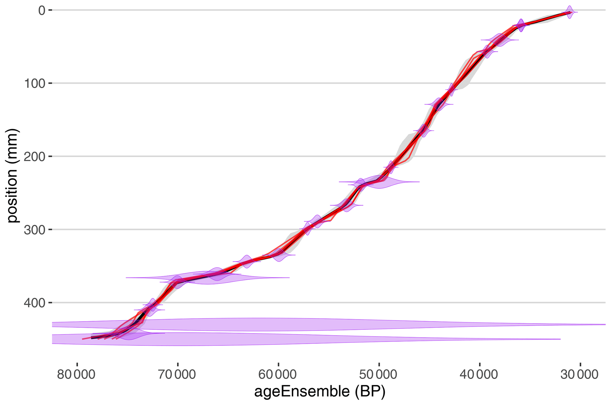
Figure 2Age–depth model generated by BChron for a speleothem from Hulu Cave. Relative age probability distributions are shown in purple. Median age–depth relationship is in black, with 50th and 95th percentile highest-density probability ranges shown in dark and light gray, respectively. Five random age–depth ensemble members are shown in red.
After an age ensemble has been added to a LiPD object, the user can visualize the ensemble time series using the plotTimeseriesEnsRibbons and plotTimeseriesEnsLines functions. GISP2 δ18O is plotted with age uncertainty, using both functions, in Fig. 3.
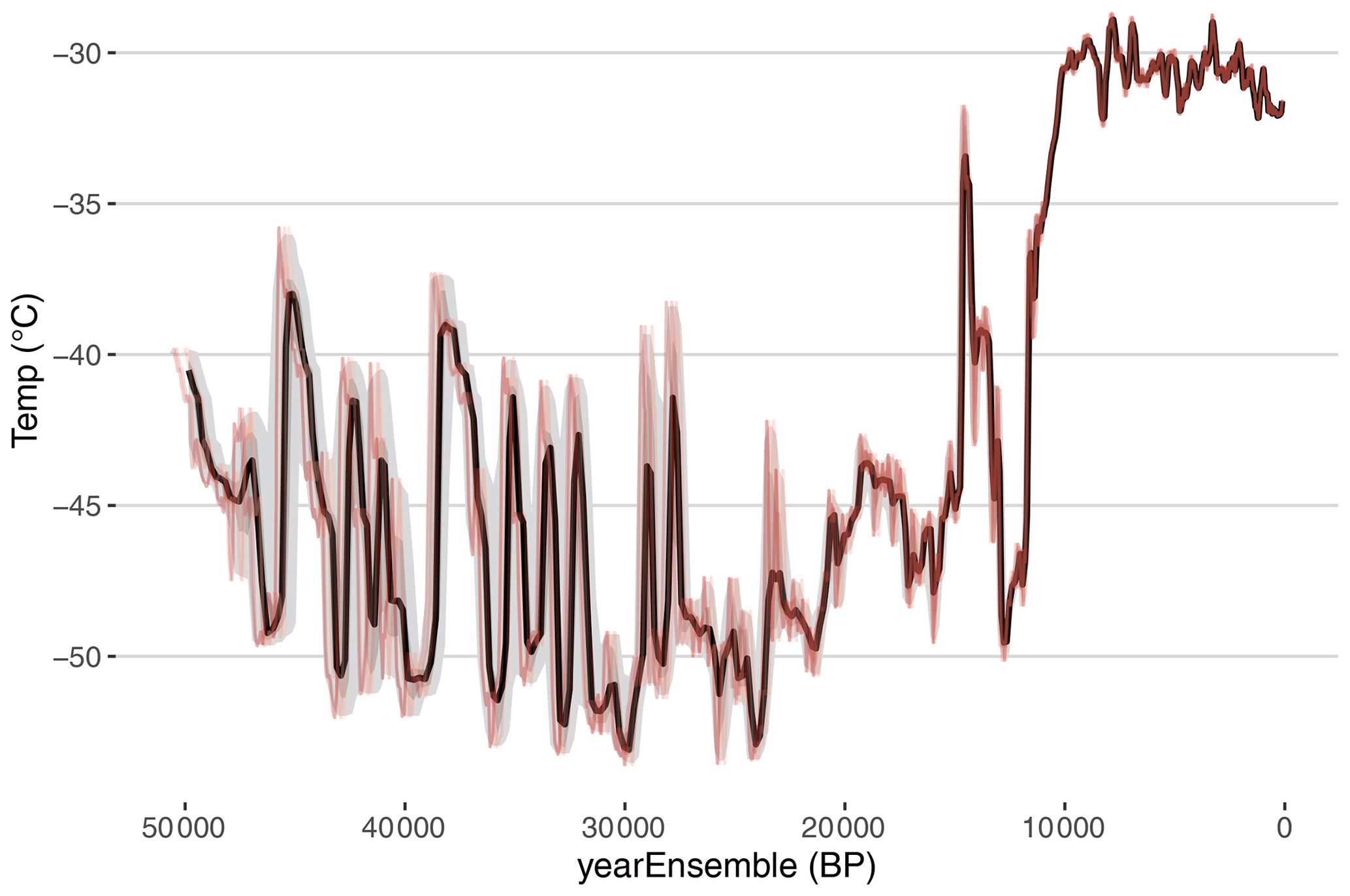
Figure 3Impact of age uncertainty on reconstructed temperature at GISP2 over the past 50 000 years. The median ensemble member is shown in black, with the 50 % and 95 % highest-density probability ranges shown in dark and light gray, respectively. Five random age-uncertain temperature ensemble members are shown in red.
5.2 Abrupt climate change in Greenland and China
Now that the user has generated age ensembles for the two datasets, they wish to see if a correlation between the two datasets is robust to the age uncertainty modeled here.
On multi-millennial timescales, the two datasets display such similar features that the well-dated Hulu Cave record, and other similar records from China and Greenland, has been used to argue for atmospheric teleconnections between the regions and support the independent chronology of GISP2 (Wang et al., 2001).
In this use case, we revisit this relation quantitatively and use the age models created above, as well as geoChronR's corEns function, to calculate the impact of age uncertainty on the correlation between these two iconic datasets.
Because these datasets are not normally distributed, we use Spearman's rank correlation to avoid the assumption of linearity.
Kendall's tau method, or Pearson correlation used after gaussianizing the input (the geoChronR default), is also a reasonable option that in most cases, including this one, produces comparable results.
Any correlation approach to address this question is, in many ways, simplistic.
Correlating the two age-uncertain datasets will characterize the relationship but ignores ancillary evidence that may support a mechanistic relationship between two time series.
Still, it illustrates how age uncertainty can affect apparent alignment between two datasets, which is the purpose of this example.
Here, we calculate correlations during the period of overlap in 200-year steps, determining significance for each pair of ensemble members while accounting for autocorrelation. geoChronR includes four built-in approaches to estimate the significance of correlations (Sect. 3.1). Here, we examine the correlation results as histograms, with color shading to highlight significance, for each of the three methods that include a correction for autocorrelation (Fig. 4). The r values are the same for all the results; only the assessment of significance changes. The two time series exhibit consistently negative correlations, although 30.8 % of the ensemble members are positive. In this example, the isopersistent approach finds the most significant correlations, with 7.8 % significant ensemble members, and 0.8 % remain significant after adjusting for false discoveries. In this instance, the isospectral approach is more conservative, with only 0.7 % significant members, none of which remain significant with FDR. Lastly, the effective sample size approach of Dawdy and Matalas (1964) is most conservative, finding no significant correlations.
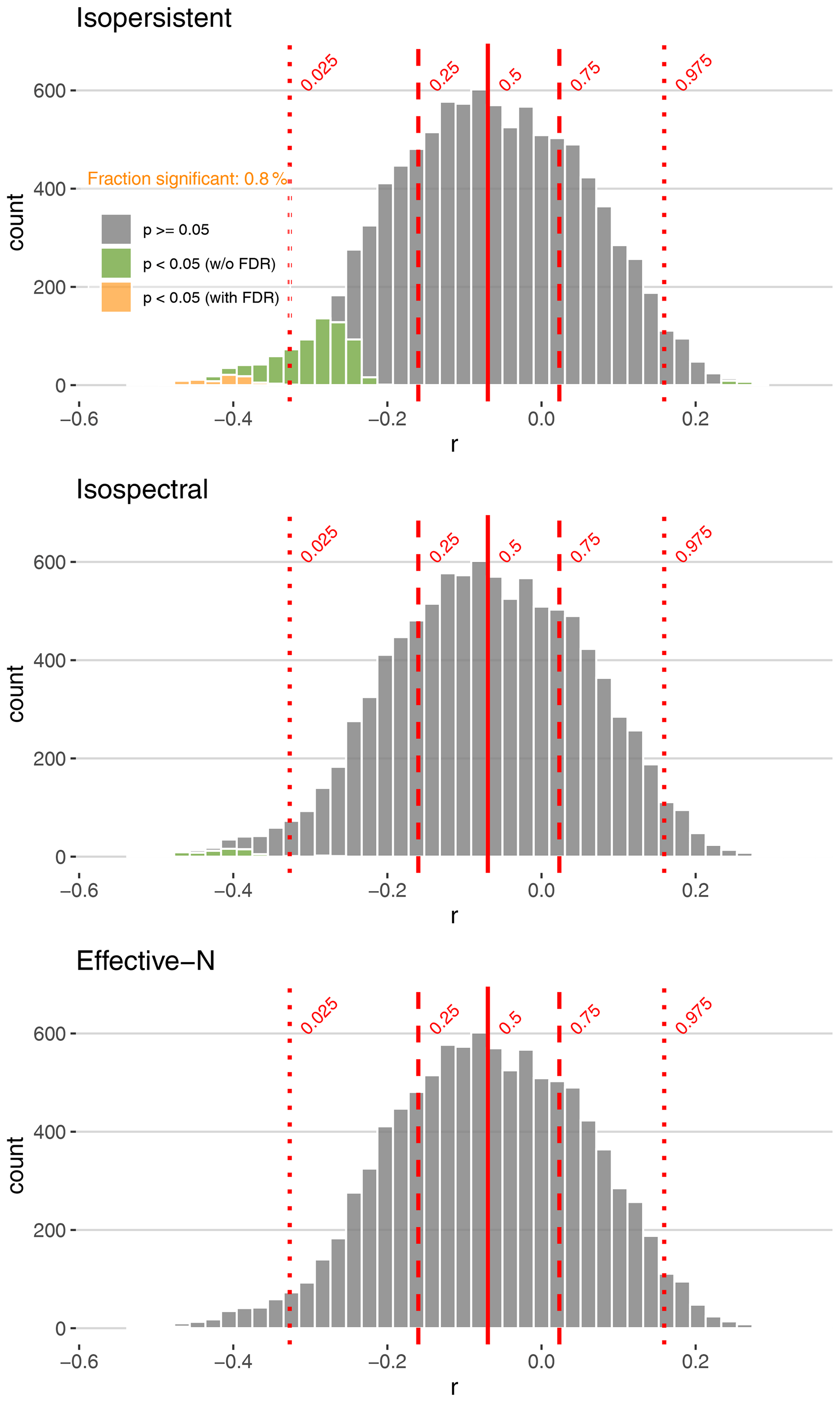
Figure 4Distribution of age-uncertain correlation between Hulu Cave speleothem and GISP2 ice core δ18O. Significant (insignificant) correlations are shown in green (gray). Correlations that remain significant after adjusting for false discovery rate (FDR) are shown in orange. Quantiles of the distribution are indicated by vertical red lines.
As mentioned above, there are many reasons to believe that there are teleconnections that link Greenland temperatures to the dynamic monsoon circulation in Asia, especially during abrupt climate changes during glacial periods (e.g., Liu et al., 2013; Duan et al., 2016; Zhang et al., 2019). Furthermore, this question has been deeply investigated with large compilations of speleothem data (Corrick et al., 2020) and improved ice-core chronologies (e.g., Andersen et al., 2006; Wolff et al., 2010). Yet this simple correlation exercise does not affirm such a link, and we offer several reason why this may be the case.
We first note that evaluating the significance of age-uncertainty correlation remains somewhat subjective, as there is no theoretical justification for what fraction of ensemble correlation results should be expected to pass such a significance test. Indeed, two correlated time series, when afflicted with age uncertainty, will commonly return some fraction of insignificant results when random ensemble members are correlated against each other. The frequency of these “false negatives” depends on the structure of the age uncertainties and the time series and will vary to some extent by random chance. One way to get a sense of the vulnerability of a time series to false negatives is to perform an age-uncertain correlation of a dataset with itself. It is appropriate to consider the results of this analysis as a best-case scenario and to consider the correlation results in this light. For illustration, we perform this calculation with the Hulu Cave δ18O record (Fig. 5).

Figure 5Distribution of age-uncertain correlation between Hulu Cave speleothem δ18O and itself, treating the age uncertainty as if it was independent. Conventions are as in Fig. 4.
The impact of age uncertainty on the correlation of this record is apparent; even when correlated against itself, only 3.5 % of the ensembles have r values greater than 0.9, and the median correlation is 0.8. However, all of the correlations remain significant, even after accounting for autocorrelation, indicating that age uncertainty and the structure of the time series does not preclude the possibility of significant correlations.
Second, correlations are spectrally blind: they lump together all timescales without regard for the dynamics that govern them. Because dynamical systems with large spatial scales tend to have long timescales as well, it is natural to expect that the GISP2 and Hulu records may vary in concert over millennial-scale events but not necessarily shorter ones. Lastly, since age uncertainties will disproportionately affect high-frequency oscillations (e.g., Comboul et al., 2014), they would obfuscate such correlations even in perfectly synchronous records.
If the goal is to align features of interest, one solution would be to extract such features via singular spectrum analysis (Vautard and Ghil, 1989; Vautard et al., 1992), then correlate such features only using the tools above. Another approach is to test for the synchronicity of abrupt events explicitly. Blaauw et al. (2010) used this approach, calculating “event probabilities” for specific time intervals between individual records, then calculating the probability of synchronous changes in two records as the product of these two probabilities for each interval. Yet another solution would be to use dedicated methods from the time series alignment (e.g., dynamic time warping) literature.
Generally, age uncertainties obscure relationships between records, while in rare cases creating the appearance of spurious correlations. It is appropriate to think of the ensemble correlation results produced by geoChronR as a first-order estimate of the age-uncertain correlation characteristics between time series rather than a binary answer to the question of whether these two datasets are significantly correlated. However, as a rule of thumb, if more than half of the ensemble correlation results are significant, it is reasonable to characterize that correlation as robust to age uncertainty.
5.3 Age-uncertain calibration
A natural extension of ensemble correlation is ensemble regression, for which a common use case is calibrating a paleoenvironmental proxy “in time” by regressing it against an instrumental series using a period of overlapping measurements (Grosjean et al., 2009). We illustrate this by reproducing the results of Boldt et al. (2015), who calibrated a spectral reflectance measure of chlorophyll abundance, relative absorption band depth (RABD), to instrumental temperature in northern Alaska. For each iteration in the analysis, a random age ensemble member is chosen and used to bin the RABD data onto a 3-year interval. The instrumental temperature data, here taken from the nearest grid cell of the NASA Goddard Institute for Space Studies (GISS) Surface Temperature Analysis (GISTEMP) reanalysis product (Hansen et al., 2010), are also binned onto the same timescale, ensuring temporal alignment between the two series. geoChronR then fits an ordinary least squares model and then uses that model to “hindcast” temperature values from 3-year binned RABD data back in time. This approach propagates the age uncertainties both through the regression (model fitting) and prediction process.
The function plotRegressEns produces multiple plots that visualize the key results of age-uncertain regression and additionally creates an overview “dashboard” that showcases the key results (Fig. 6). The first row of Fig. 6 illustrates the impact of age uncertainty on the regression modeling.
In this example, the distributions of the modeled parameters (the slope and intercept of the regression equation) show pronounced modes near 150 ∘C−1 and −130 ∘C, respectively, but with pronounced tails that include models with much lower slopes. This is also apparent in the scatterplot in the central panel of the top row, which illustrates the distribution of modeled relationships.
Although the tendency for robust relationships is clear, models with slopes near zero also occur, suggesting that in this use case, age uncertainty can effectively destroy the relationship with instrumental data.
The impact of this variability in modeled parameters, as well as the effects of age uncertainty on the timing of the reconstruction are shown in the bottom panel of Fig. 6.
The results shown here are consistent with those presented by Boldt et al. (2015), and we refer readers to that study for a full discussion of the implications of their results.
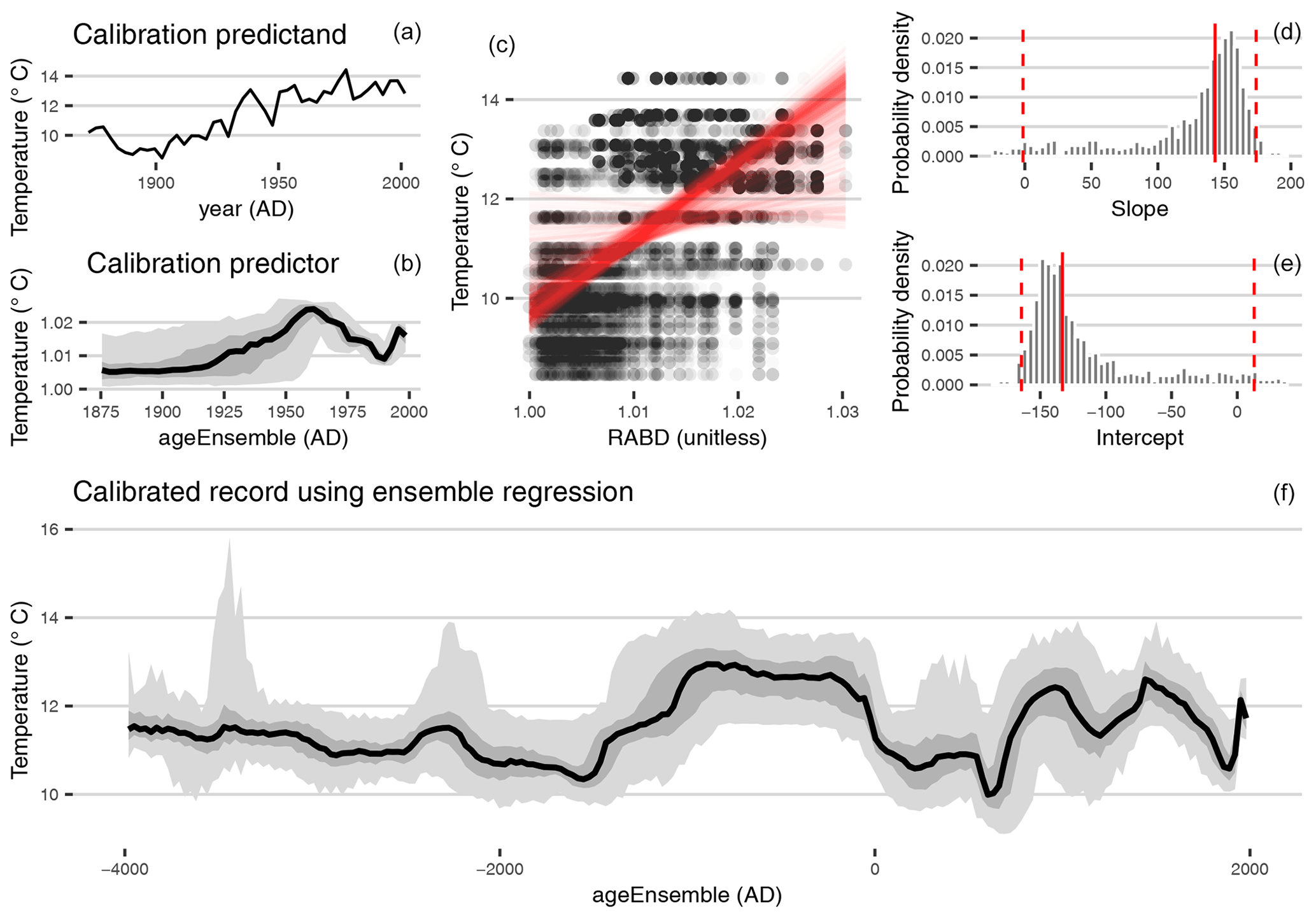
Figure 6Results of ensemble regression. (a) The calibration-in-time predictor and predictand. The predictand shows the effect of age uncertainty, the median is shown in black, and the 50 % and 95 % highest-probability density regions are shown in dark and light gray, respectively. (b) Scatterplot showing the relation between RABD and temperature. Points from 100 age ensemble members are plotted with transparency to highlight data overlap. Ensemble regression models are plotted with semi-transparent red lines. (d, e) Distribution of regression model slope (d) and intercepts (e). Vertical red lines show the 50th (solid), 2.5th and 97.5th (dashed) percentiles. (f) Reconstructed temperature using age ensembles and regression model ensembles. The median estimate is shown in black, and the 50 % and 95 % highest-probability density regions are shown in dark and light gray, respectively.
We note that there are use cases where regressing one age-uncertain variable onto another is called for, and regressEns supports such applications as well.
5.4 Arctic spatiotemporal variability over the Common Era
The previous use cases have highlighted age-uncertain analyses at one or two locations. Yet quantifying the effects of age uncertainty can be even more impactful over larger collections of sites. Here, we showcase how to use geoChronR to perform age-uncertain PCA (Sect. 3.3). When seeking to analyze a large collection of datasets, the first, and often most time-intensive, step is to track down, format, and standardize the data. Fortunately, the emergence of community-curated standardized data collections (e.g., PAGES2K Consortium, 2013; Emile-Geay et al., 2017; Kaufman et al., 2020b; Konecky et al., 2020) can greatly simplify this challenge. In this example, we examine the Arctic 2k database (McKay and Kaufman, 2014) and use geoChronR and the LiPD utilities to filter the data for temperature-sensitive data from the Atlantic Arctic with age ensembles relevant to the past 2000 years.
Once filtered, the data can be visualized using plotTimeseriesStack, which is an option to quickly plot all of the time series, on their best-estimate age models, aligned on a common horizontal timescale (Fig. 7). Although all of the datasets are relevant to Arctic temperatures over the past 2000 years, they span different time intervals, with variable temporal resolution. It is also clear that there is a lot of variability represented within the data, but it is difficult to visually extract shared patterns of variability.
Ensemble PCA identifies the modes of variability that explain the most variance within a dataset, while accounting for the impact of age uncertainty.

Figure 7Temperature-sensitive time series from the Atlantic Arctic in McKay and Kaufman (2014), arranged vertically by variable. Each time series is shown on its own scale to the right or left of each time series.
As in correlation and regression, aligning the data onto a common timescale is required for ensemble PCA. All but two of these datasets are annually resolved, and the other two have 5-year resolution, so it is reasonable to average these data into 5-year bins. Furthermore, since many of the records do not include data before 1400 CE, we only analyze the period from 1400 to 2000 CE. The data are now prepared for the ensemble PCA calculation, following a few choices in methodology and parameters. Because the data analyzed here have variable units, and we are not interested in the magnitude of the variance (only the relative variability between the datasets), we choose to use a correlation, rather than covariance, matrix. Next, we choose the number of components to estimate. After the analysis, a scree plot is used to determine the number of significant components. We want to estimate several more components than we anticipate will be meaningful. For this use case, we estimate eight components.
We now conduct the ensemble PCA, including null hypothesis testing, for 100 ensemble members. For a final analysis, 1000 ensemble members is standard; however, the analysis can be time consuming and 100 members is appropriate for exploratory analyses. First, we plot the ensemble variance explained results for the data and the null hypothesis as a scree plot (Fig. 8). This represents how the variance explained by each component declines with each mode for both the data and the null hypothesis. Due to age uncertainty, the resulting variance explained is a distribution, which we compare to the 95th quantile of the null hypothesis ensemble. Figure 8 indicates that the first two components are clearly distinguished from the null. The third component is borderline, with the variance explained by the median of the ensemble near the null. Therefore, we will focus our investigation on the first two modes.
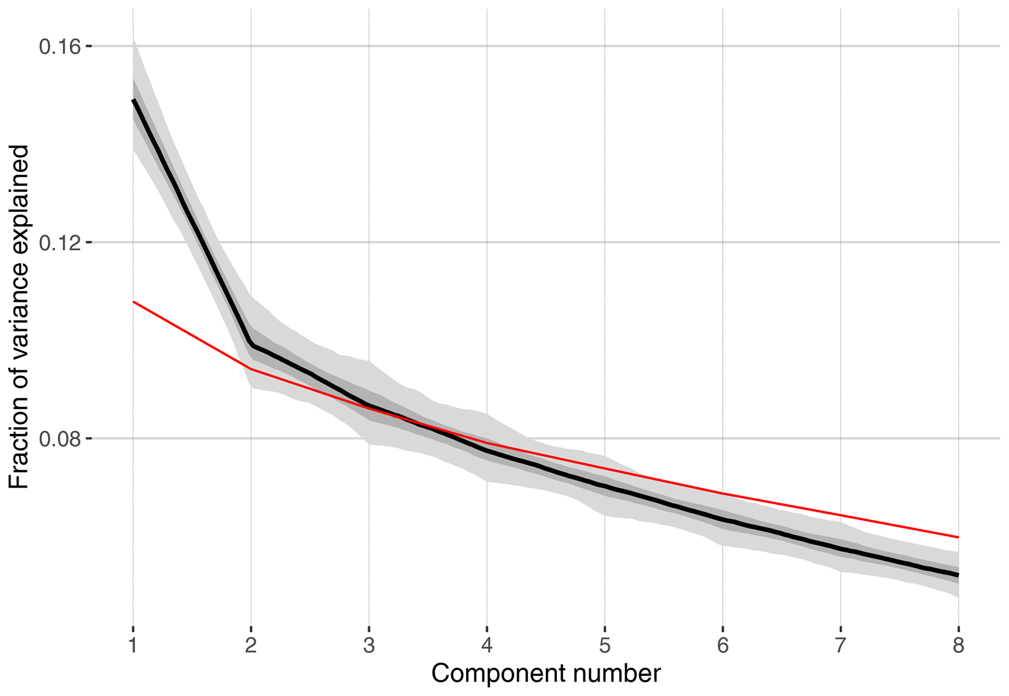
Figure 8Ensemble PCA scree plot showing the fraction of variance explained as a function of component (or eigenvalue) number. The ensemble PCA results for the data have uncertainty due to age uncertainty. The median is shown in black, and the 50 % and 95 % highest-probability density regions are shown in dark and light gray, respectively. The 95th percentile of the null hypothesis test is shown in red.
The spatial and temporal results of the first two principal components are shown in Fig. 9. The first PC is dominated by consistently positive loadings across the North Atlantic, suggesting that this is a regionally persistent mode of variability and indicating that none of the datasets are negatively correlated with this mode. The corresponding time series shows multidecadal variability, with values declining until the 18th century, before increasing into the 20th century. Based on the region-wide coherence of the loading pattern and the similarity of the time series to regional temperature reconstructions (Hanhijärvi et al., 2013; McKay and Kaufman, 2014; Werner et al., 2018), the first PC likely reflects the primary pattern of regional temperature variability. Notably, the uncertainties in the PC1 time series, and the loadings in the spatial pattern, are generally small. This, combined with the large amount of variance explained by PC1 relative to the null hypothesis (Fig. 8), suggests this is a significant mode of variability that is robust to age uncertainty. This makes intuitive sense, since the primary features of this pattern are century-long trends in temperature, a timescale that substantially exceeds the age uncertainty in these data (McKay and Kaufman, 2014).
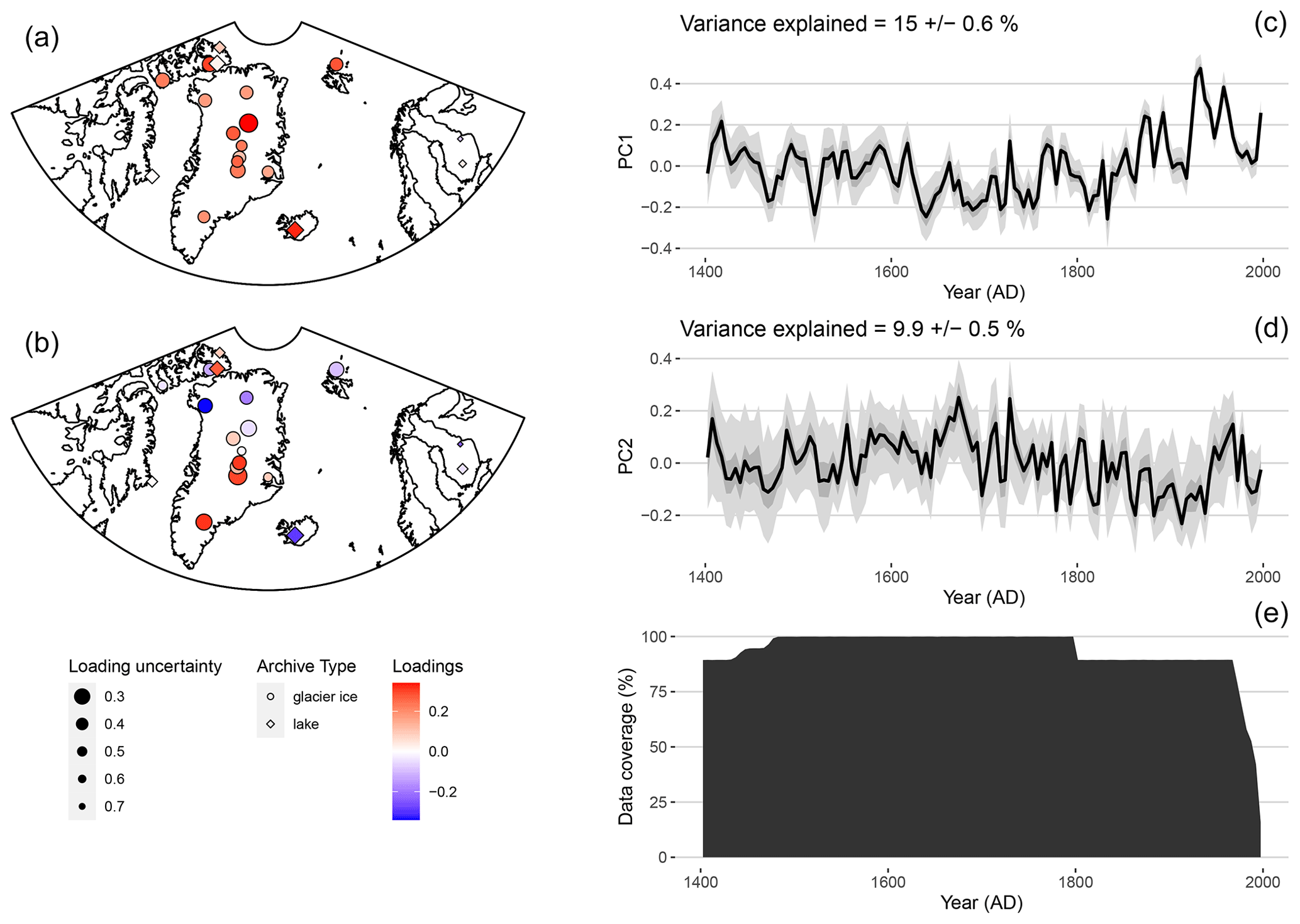
Figure 9The spatial loading pattern (a, b) and time series (c, d, e) for the first principal component shown in panels (a, c). The results for the second PC are shown in panels (b, d). The data density through time is shown in panel (e). For the maps, the median loadings of the ensemble are shown by the color scale, and the standard deviation of the loadings across ensemble members is depicted by the size of the markers, with larger markers showing smaller uncertainties. For the time series plots, the median of the ensemble is shown in black, and the 50 % and 95 % highest-probability density regions are shown in dark and light gray, respectively.
The second PC shows considerable more variability in its spatial loading pattern and a larger impact of age uncertainty. Generally, the loadings suggest a north–south dipole over Greenland for this mode, with positive loadings present in much of southern Greenland, with negative loadings in present in much of the northern part of the region. There is a much larger impact of age uncertainty on the loadings in PC2 than in PC1, illustrated by the size of the markers on the map, which are inversely related to the standard deviation of the loadings across the ensemble PCA results, such that smaller markers indicate larger uncertainties. The PC2 time series includes more multidecadal variability than PC1 and is more impacted by age uncertainty. A key feature of the time series is a peak in values in the late 20th century, which occurs after the pronounced peak in PC1. This suggests that unlike the mid-20th century peak in warming apparent in most of the data, this later warming was dominated by contributions from southern Greenland and counterbalanced by a decline in values in the northern Atlantic Arctic.
5.5 Orbital-scale variability in a deep-sea core
To illustrate the use of spectral analysis in geoChronR, we consider a use case where the user seeks to identify the relative energy of oscillations at orbital (Milankovitch) periodicities in a deep-sea sediment core and quantify the impact of age uncertainties on this assessment. Here, we use a benthic paleotemperature record derived from the International Ocean Drilling Project (IODP) core 846 (Mix et al., 1995; Shackleton, 1995), which covers the past 4.7 million years. For this assessment, we use an updated age model generated outside geoChronR, via alignment to the benthic δ18O stack of Lisiecki and Raymo (2005) using the hidden Markov model (HMM) match algorithm (Lin et al., 2014; Khider et al., 2017). HMM match is a probabilistic method that generates an ensemble of 1000 possible age models compatible with the chronostratigraphic constraints; this ensemble was archived as a table in the associated LiPD file (http://lipdverse.org/geoChronR-examples/ODP846.Lawrence.2006.lpd, last access: 22 February 2021), making it accessible to geoChronR.
First, we use plotTimeseriesEnsRibbons to visualize temperature, and the impact of age uncertainty, over the past 5 million years (Fig. 10).
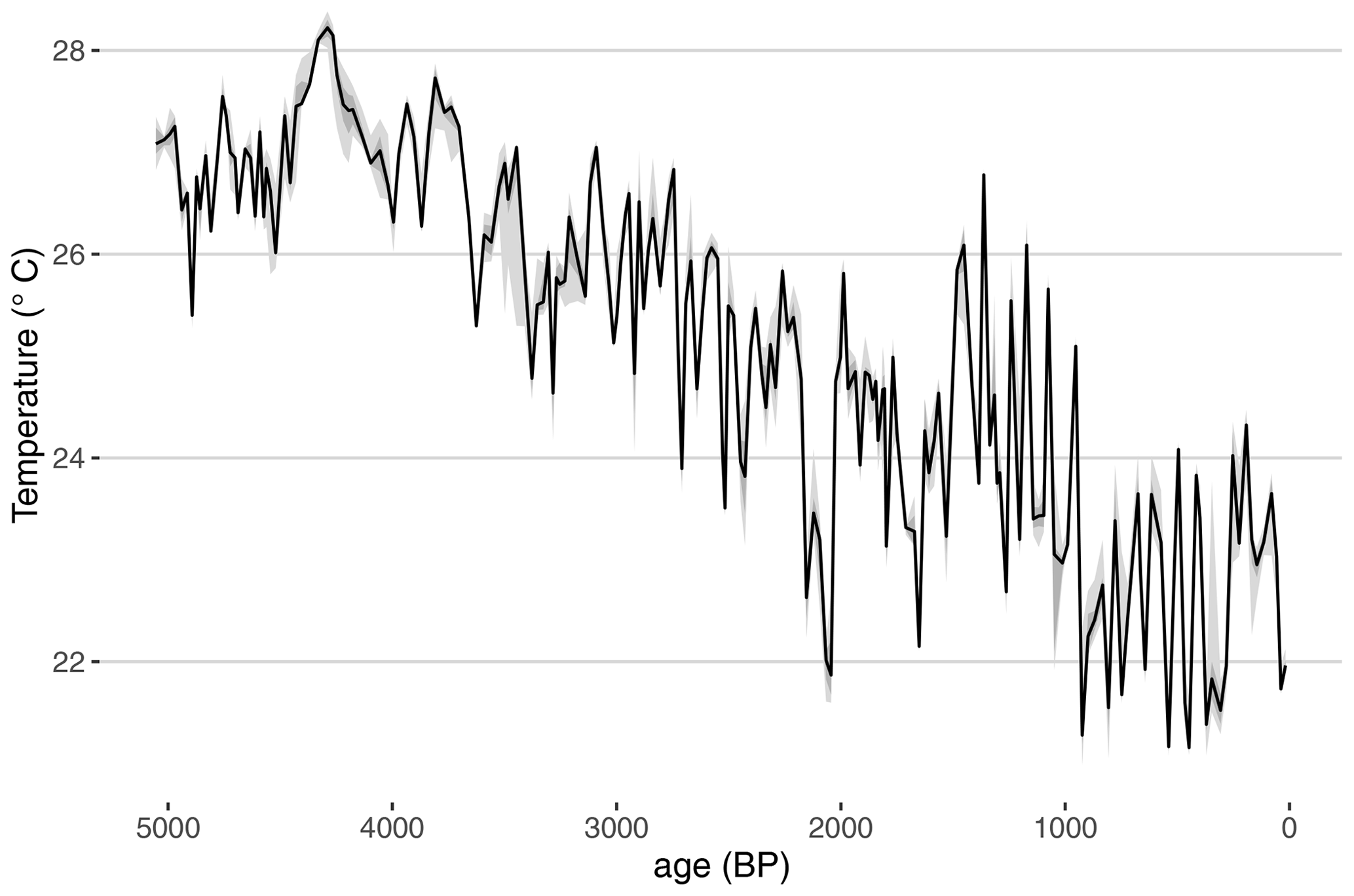
Figure 10Temperature reconstruction from IODP 846. The median ensemble member is shown in black, with the 50 % and 95 % highest-density probability ranges shown in dark and light gray, respectively.
The record displays three salient features:
-
a long-term cooling trend characteristic of the late Neogene and Quaternary climate,
-
quasi-periodic oscillations (the Pleistocene ice ages), and
-
non-stationary behavior, related to the well-known mid-Pleistocene transition from a “41k world” to a “100k world” somewhere around 0.8 Ma (Paillard, 2001; Lisiecki and Raymo, 2005; Ahn et al., 2017).
For tractability, let us focus on the last million years, which cover the Quaternary era. Over this interval, the time increments (Δt) are sharply peaked around 2.5 ka, spanning 0 to about 7.5 ka. From this point, there are two ways to proceed: (1) use methods that explicitly deal with unevenly spaced data or (2) interpolate to a regular grid and apply methods that assume even spacing (see Sect. 3.4). Here, we will use both approaches and highlight two of the four spectral methods implemented in geoChronR: REDFIT and MTM.
We use the computeSpectraEns function to calculate the spectra for 1000 ensemble members using the REDFIT approach (Fig. 11). It is clear that the data contain significant energy (peaks) near, but not exactly at, the Milankovitch periodicities (100, 41, 23, and 19 ka). These periodicities, particularly those associated with eccentricity (100 ka) and precession (23 and 19 ka), rise above the null hypothesis (the 95 % quantile from an autoregressive process of first order; see Mudelsee et al., 2009).
The obliquity periodicity is relatively weak, reaching just below the AR(1) benchmark.
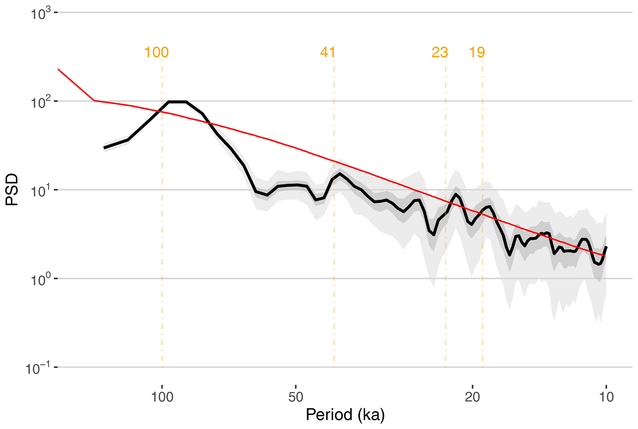
Figure 11REDFIT spectrum for IODP 846. Median spectrum is shown in black, with the 50 % and 95 % highest-density probability ranges shown in dark and light gray, respectively. Periodicities of interest (in ka) are shown in orange.
The Lomb–Scargle periodogram used by REDFIT is a common way to deal with unevenly spaced time series, but like all periodograms, it is inconsistent: the uncertainty about the spectral density at each frequency does not decrease with the number of observations. This is mitigated somewhat with the application of Welch's overlapping segment averaging, whose parameter choices (number of widows and degree of overlap) are ad hoc. In contrast, MTM (Thomson, 1982) is an optimal estimator, which is consistent (the more observations, the better constrained the spectral density), and its parameter choice is explicit. Formally, MTM optimizes the classic bias-variance trade-off inherent to all statistical inference.
It does so by minimizing spectral leakage outside of a frequency band with half bandwidth equal to pfR, where is the Rayleigh frequency, Δt is the sampling interval, N the number of measurements, and p is the so-called “time–bandwidth product” (Ghil et al., 2002).
p can only take a finite number of values: all multiples of 0.5 between 2 and 4. A larger p means lower variance (i.e., less uncertainty about the power) but broader peaks (i.e., a lower spectral resolution), synonymous with more uncertainty about the exact location of the peak. So while MTM might not distinguish between closely spaced harmonics, it is much less likely to identify spurious peaks, especially at high frequencies. Several formal tests have been devised for both methods, allowing us to ascertain the significance of spectral peaks under reasonably broad assumptions. We show how to use MTM's “harmonic F test” below. However, classic MTM can only handle evenly spaced data. Since the data are close to being evenly spaced, it is reasonable to interpolate them using standard methods. Both interpolation and MTM are implemented with the astrochron (Meyers, 2014) package, which geoChronR employs.
To the spectral distribution itself we can add the periods identified as significant by MTM's F ratio test. geoChronR estimates this by computing the fraction of ensemble members that exhibit a significant peak at each frequency. One simple criterion for gauging the level of support for such peaks given age uncertainties is to pick out those periodicities that are identified as significant above a certain threshold (say, more than 50 % of the time). For consistency with REDFIT, we define the null as an AR(1) process fit to the data, but geoChronR supports two other nulls: a power-law null and a fit to the spectral background (Mann and Lees, 1996).
Both follow the astrochron implementation.
Figure 12 shows a few differences between the REDFIT estimate (Fig. 11) and the MTM estimate. First, this ensemble of spectra exhibits a clear power-law behavior from periods of 5 to 100 ka, which in this log–log plotting convention manifests as a linear decrease. This is part of the well-documented “continuum of climate variability” (Huybers and Curry, 2006; Zhu et al., 2019), which is conspicuously absent from the Lomb–Scargle (REDFIT) estimate, known to be heavily biased in its estimate of the spectral background (Schulz and Mudelsee, 2002).
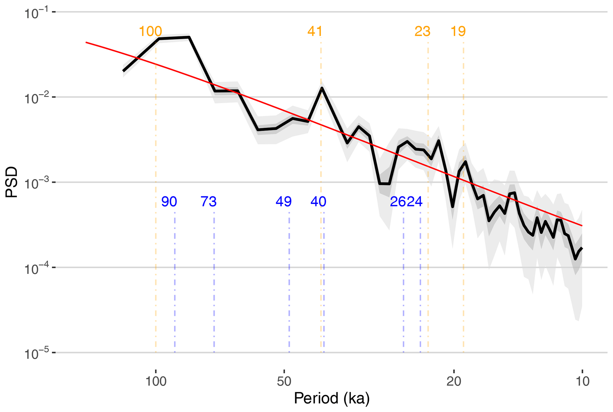
Figure 12MTM spectrum for IODP 846. Median spectrum is shown in black, with the 50 % and 95 % highest-density probability ranges shown in dark and light gray, respectively. Periodicities of interest (in ka) are shown in orange, and the periodicities identified as significant by the F ratio test are shown in blue.
Secondly, the MTM version with this time–bandwidth product is sharper than REDFIT, with more well-defined peaks, particularly for the obliquity period (41 ka), which clearly exceeds the 95 % confidence limit.
Here, it is helpful to take a step back and contemplate our null hypothesis of AR(1) background and the possibility that we might be underestimating the lag-1 autocorrelation, hence making the test too lenient.
More importantly, the presence of scaling behavior (power-law decrease) suggests that this should be a more appropriate null against which to test the emergence of spectral peaks. In geoChronR, this can be done by specifying mtm_null = "power_law" in the function call.
Using a power-law null hypothesis makes a few cycles appear non-significant, but many remain (not shown). However, carrying out a test simultaneously at many periodicities is bound to affect assessments of significance via the multiple comparisons problem (Vaughan et al., 2011). In addition, sedimentary processes (and many processes in other proxy archives) tend to smooth out the signal over the depth axis, making comparisons at neighboring frequencies highly dependent (Meyers, 2012).
One solution is to use predictions made by a physical model about the frequency and relative amplitude of astronomical cycles (Meyers and Sageman, 2007). This approach, however, is not be applicable to all spectral detection problems. Ultimately, the user must think deeply about the null hypothesis and the most sensible way to test it. Readers are invited to consider the literature for a deeper exploration of these questions (e.g., Vaughan et al., 2011; Meyers, 2012, 2015; Meyers and Malinverno, 2018).
As with all statistical analyses in the paleoenvironmental sciences and geosciences, there are no universal solutions or parameter choices. The approaches implemented in geoChronR, especially with default choices, are best considered as exploratory tools. They are intended to provide insight into the impacts of age uncertainty on power spectra and to help users tailor their null hypotheses to their scientific questions.
This article introduced an open-source R package providing user-friendly access to common age-modeling tools in the paleoenvironmental sciences and geosciences, using them to perform common tasks and intuitively visualize the results. geoChronR leverages the power of ensembles to propagate chronological uncertainties to subsequent stages of analysis. While the approach does not address all aspects of uncertainty, it does provide key insights into which results are robust to chronological uncertainty, and which are not.
Although the code was designed to perform a few common tasks in a concise and intuitive way, geoChronR also has the underlying infrastructure to support customized analyses for users seeking to address more complex questions (e.g., Thomas et al., 2018). At this stage, the paleoenvironmental and geoscientific communities are still only scratching the surface of age-uncertain analysis, so many extensions are possible. We hope this article encourages the community to extend and expand this open-source package to achieve many more scientific goals than we could possibly enumerate here.
One potentially useful application of geoChronR is age-model intercomparison, as it provides a standardized platform upon which methods can be readily tested and compared. Scholz et al. (2012) and Parnell et al. (2011) performed comparisons of some of methods employed, coming to somewhat different conclusions. More recently, Trachsel and Telford (2017) compared several of the methods included in geoChronR (including OxCal, BChron, and Bacon) on a well-dated, varved lake chronology. They conclude that “All methods produce mean age–depth models that are close to the true varve age, but the uncertainty estimation differs considerably among models”. There is thus more to be done to document, benchmark, and understand the effects of these various modeling choices, and having multiple approaches available in a standardized platform should facilitate much larger-scale benchmarking efforts.
Looking forward, we suggest that the next major direction for age-uncertain analysis may not be technical but philosophical in nature. Thus far, the community has focused on quantifying the range of possibilities presented by age uncertainty on a record-by-record basis, and geoChronR has followed that approach. In the future, one could envision developing approaches that leverage information from neighboring records. While idealized studies have laid the groundwork for using common forcings and/or covariance structures to do so (Werner and Tingley, 2015), much remains to be done to develop such a multi-site assessment of chronological uncertainties.
geoChronR is open-source community software and has benefited substantially from multiple contributors and input from early adopters and workshop participants. We continue to welcome feedback and strongly encourage contributions and enhancements via the GitHub issue tracker (https://github.com/nickmckay/geoChronR/issues, last access: 22 February 2021).
All of the code used in geoChronR is open and available at https://github.com/nickmckay/geochronr (last access: 22 February 2021, McKay et al., 2021b), and we welcome contributions and extensions to the package. The R Markdown code used to create this paper is available at https://github.com/nickmckay/geochronr-paper (last access: 22 February 2021, McKay et al., 2021a).
All of the data used in this paper are publicly archived and available as LiPD files at http://lipdverse.org/geoChronR-examples/ (last access: 22 February 2021, McKay, 2021).
NPM and JEG conceived the idea for geoChronR. NPM led the development of the geoChronR package and the paper. JEG led the implementation of the spectral analysis capabilities in geoChronR and their description in the paper. DK led the implementation of BChron in geoChronR and its description in the paper. All authors contributed to writing and revising the paper.
The authors declare that they have no conflict of interest.
The software described here is provided under the MIT License, and is provided “as is”, without warranty of any kind, express or implied, including but not limited to the warranties of merchantability, fitness for a particular purpose and noninfringement. In no event shall the authors or copyright holders be liable for any claim, damages or other liability, whether in an action of contract, tort or otherwise, arising from, out of or in connection with the software or the use or other dealings in the software.
We thank the participants of the 2016 and 2017 geoChronR workshops for their contributions to the testing and design, which dramatically improved this package.
This research has been supported by the National Science Foundation, Directorate for Geosciences (grant no. EAR-1347221).
This paper was edited by Noah M. McLean and reviewed by two anonymous referees.
Ahn, S., Khider, D., Lisiecki, L. E., and Lawrence, C. E.: A probabilistic Pliocene–Pleistocene stack of benthic δ18O using a profile hidden Markov model, Dynamics and Statistics of the Climate System, 2, dzx002, https://doi.org/10.1093/climsys/dzx002, 2017. a
Alley, R. B.: Ice-core evidence of abrupt climate changes, P. Natl. Acad. Sci. USA, 97, 1331–1334, 2000. a
Anchukaitis, K. J. and Tierney, J. E.: Identifying coherent spatiotemporal modes in time-uncertain proxy paleoclimate records, Clim. Dynam., 41, 1291–1306, 2013. a, b, c
Andersen, K. K., Svensson, A., Johnsen, S. J., Rasmussen, S. O., Bigler, M., Röthlisberger, R., Ruth, U., Siggaard-Andersen, M. L., Steffensen, J. P., Dahl-Jensen, D., and Vinther, B. M.: The Greenland ice core chronology 2005, 15–42 ka, Part 1: constructing the time scale, Quaternary Sci. Rev., 25, 3246–3257, 2006. a
Balco, G., Briner, J., Finkel, R. C., Rayburn, J. A., Ridge, J. C., and Schaefer, J. M.: Regional beryllium−10 production rate calibration for late-glacial northeastern North America, Quat. Geochronol., 4, 93–107, https://doi.org/10.1016/j.quageo.2008.09.001, 2009. a
Becker, R. A., Wilks, A. R., Minka, R. B. T. P., and Deckmyn, A.: maps: Draw Geographical Maps, R package, version 3.3.0, available at: https://CRAN.R-project.org/package=maps (last access: 22 February 2021), 2018. a
Benjamini, Y. and Hochberg, Y.: Controlling the False Discovery Rate: A Practical and Powerful Approach to Multiple Testing, J. Roy. Stat. Soc. B Met., 57, 289–300, 1995. a
Bhattacharya, T. and Coats, S.: Atlantic-Pacific Gradients Drive Last Millennium Hydroclimate Variability in Mesoamerica, Geophys. Res. Lett., 47, e2020GL088061, https://doi.org/10.1029/2020GL088061, 2020. a, b
Blaauw, M.: Methods and code for “classical” age-modelling of radiocarbon sequences, Quat. Geochronol., 5, 512–518, 2010. a, b, c
Blaauw, M.: Out of tune: the dangers of aligning proxy archives, Quaternary Sci. Rev., 36, 38–49, 2012. a
Blaauw, M. and Christen, J. A.: Flexible paleoclimate age-depth models using an autoregressive gamma process, Bayesian Anal., 6, 457–474, 2011. a, b, c
Blaauw, M., Christen, J., Mauquoy, D., van der Plicht, J., and Bennett, K.: Testing the timing of radiocarbon-dated events between proxy archives, Holocene, 17, 283–288, 2007. a
Blaauw, M., Wohlfarth, B., Christen, J. A., Ampel, L., Veres, D., Hughen, K. A., Preusser, F., and Svensson, A.: Were last glacial climate events simultaneous between Greenland and France? A quantitative comparison using non-tuned chronologies, J. Quaternary Sci., 25, 387–394, 2010. a
Blaauw, M., Christen, J. A., and Aquino Lopez, M. A.: rbacon: Age-Depth Modelling using Bayesian Statistics, R package, version 2.4.2, available at: https://CRAN.R-project.org/package=rbacon (last access: 22 February 2021), 2020. a, b
Boers, N., Goswami, B., and Ghil, M.: A complete representation of uncertainties in layer-counted paleoclimatic archives, Clim. Past, 13, 1169–1180, https://doi.org/10.5194/cp-13-1169-2017, 2017. a
Boldt, B. R., Kaufman, D. S., McKay, N. P., and Briner, J. P.: Holocene summer temperature reconstruction from sedimentary chlorophyll content, with treatment of age uncertainties, Kurupa Lake, Arctic Alaska, Holocene, 25, 641–650, https://doi.org/10.1177/0959683614565929, 2015. a, b, c
Bond, G., Kromer, B., Beer, J., Muscheler, R., Evans, M. N., Showers, W., Hoffmann, S., Lotti-Bond, R., Hajdas, I., and Bonani, G.: Persistent Solar Influence on North Atlantic Climate During the Holocene, Science, 294, 2130–2136, 2001. a
Bronk Ramsey, C.: Radiocarbon calibration and analysis of stratigraphy: The OxCal program, Radiocarbon, 37, 425–430, 1995. a
Bronk Ramsey, C.: Deposition models for chronological records, Quaternary Sci. Rev., 27, 42–60, 2008. a, b
Bronk Ramsey, C.: Bayesian analysis of radiocarbon dates, Radiocarbon, 51, 337–360, 2009. a
Bronk Ramsey, C., Dee, M., Lee, S., Nakagawa, T., and Staff, R. A.: Developments in the calibration and modeling of radiocarbon dates, Radiocarbon, 52, 953–961, 2010. a
Bunn, A. G.: A dendrochronology program library in R (dplR), Dendrochronologia, 26, 115–124, https://doi.org/10.1016/j.dendro.2008.01.002, 2008. a
Charreau, J., Blard, P.-H., Zumaque, J., Martin, L. C., Delobel, T., and Szafran, L.: Basinga: A cell-by-cell GIS toolbox for computing basin average scaling factors, cosmogenic production rates and denudation rates, Earth Surf. Proc. Land., 44, 2349–2365, 2019. a
Comboul, M., Emile-Geay, J., Evans, M. N., Mirnateghi, N., Cobb, K. M., and Thompson, D. M.: A probabilistic model of chronological errors in layer-counted climate proxies: applications to annually banded coral archives, Clim. Past, 10, 825–841, https://doi.org/10.5194/cp-10-825-2014, 2014. a, b, c, d, e
Corrick, E. C., Drysdale, R. N., Hellstrom, J. C., Capron, E., Rasmussen, S. O., Zhang, X., Fleitmann, D., Couchoud, I., and Wolff, E.: Synchronous timing of abrupt climate changes during the last glacial period, Science, 369, 963–969, 2020. a
Dawdy, D. R. and Matalas, N. C., 1964, Analysis of variance, covariance, and time series, in: Handbook of applied hydrology, edited by: Chow, V. T., New York, McGraw-Hill Book Co., 8-68–8-90, 1964. a, b
Dee, S., Emile-Geay, J., Evans, M. N., Allam, A., Steig, E. J., and Thompson, D. M.: PRYSM: An open-source framework for PRoxY System Modeling, with applications to oxygen-isotope systems, J. Adv. Model. Earth Sy., 7, 1220–1247, 2015. a
Deininger, M., McDermott, F., Mudelsee, M., Werner, M., Frank, N., and Mangini, A.: Coherency of late Holocene European speleothem δ18O records linked to North Atlantic Ocean circulation, Clim. Dynam., 49, 595–618, 2017. a
DeLong, K. L., Quinn, T. M., Taylor, F. W., Shen, C.-C., and Lin, K.: Improving coral-base paleoclimate reconstructions by replicating 350 years of coral variations, Palaeogeogr. Palaeocl., 373, 6–24, https://doi.org/10.1016/j.palaeo.2012.08.019, 2013. a
Duan, W., Cheng, H., Tan, M., and Edwards, R. L.: Onset and duration of transitions into Greenland Interstadials 15.2 and 14 in northern China constrained by an annually laminated stalagmite, Sci. Rep.-UK, 6, 20844, https://doi.org/10.1038/srep20844, 2016. a
Ebisuzaki, W.: A Method to Estimate the Statistical Significance of a Correlation When the Data Are Serially Correlated, J. Climate, 10, 2147–2153, https://doi.org/10.1175/1520-0442(1997)010<2147:AMTETS>2.0.CO;2, 1997. a
Eggins, S. M., Grün, R., McCulloch, M. T., Pike, A. W., Chappell, J., Kinsley, L., Mortimer, G., Shelley, M., Murray-Wallace, C. V., and Spötl, C.: In situ U-series dating by laser-ablation multi-collector ICPMS: new prospects for Quaternary Geochronology, Quaternary Sci. Rev., 24, 2523–2538, 2005. a
Emile-Geay, J. and Tingley, M.: Inferring climate variability from nonlinear proxies: application to palaeo-ENSO studies, Clim. Past, 12, 31–50, https://doi.org/10.5194/cp-12-31-2016, 2016. a
Emile-Geay, J., McKay, N. P., Kaufman, D. S., et al.: A global multiproxy database for temperature reconstructions of the Common Era, Scientific Data, 4, 170088, https://doi.org/10.1038/sdata.2017.88, 2017. a
Falster, G., Tyler, J., Grant, K., Tibby, J., Turney, C., Löhr, S., Jacobsen, G., and Kershaw, A. P.: Millennial-scale variability in south-east Australian hydroclimate between 30 000 and 10 000 years ago, Quaternary Sci. Rev., 192, 106–122, 2018. a
Foster, G.: Wavelets for period analysis of unevenly sampled time series, Astron. J., 112, 1709–1729, https://doi.org/10.1086/118137, 1996. a
Ghil, M., Allen, R. M., Dettinger, M. D., Ide, K., Kondrashov, D., Mann, M. E., Robertson, A., Saunders, A., Tian, Y., Varadi, F., and Yiou, P.: Advanced spectral methods for climatic time series, Rev. Geophys., 40, 1003–1052, 2002. a, b, c, d
Grosjean, M., von Gunten, L., Trachsel, M., and Kamenik, C.: Calibration-in-time: Transforming biogeochemical lake sediment proxies into quantitative climate variables, Pages News, 17, 108–110, 2009. a, b
Haam, E. and Huybers, P.: A test for the presence of covariance between time-uncertain series of data with application to the Dongge Cave speleothem and atmospheric radiocarbon records, Paleoceanography, 25, PA2209, https://doi.org/10.1029/2008PA001713, 2010. a
Hanhijärvi, S., Tingley, M. P., and Korhola, A.: Pairwise comparisons to reconstruct mean temperature in the Arctic Atlantic Region over the last 2000 years, Clim. Dynam., 41, 2039–2060, 2013. a
Hansen, J., Ruedy, R., Sato, M., and Lo, K.: Global surface temperature change, Rev. Geophys., 48, RG4004, https://doi.org/10.1029/2010RG000345, 2010. a
Haslett, J. and Parnell, A.: A simple monotone process with application to radiocarbon-dated depth chronologies, J. R. Stat. Soc. C-Appl., 57, 399–418, https://doi.org/10.1111/j.1467-9876.2008.00623.x, 2008. a
Heegaard, E., Birks, H. J. B., and Telford, R. J.: Relationships between calibrated ages and depth in stratigraphical sequences: an estimation procedure by mixed-effect regression, Holocene, 15, 612–618, 2005. a
Hu, J., Emile-Geay, J., and Partin, J.: Correlation-based interpretations of paleoclimate data – where statistics meet past climates, Earth Planet. Sc. Lett., 459, 362–371, https://doi.org/10.1016/j.epsl.2016.11.048, 2017. a, b, c
Huybers, P. and Curry, W.: Links between annual, Milankovitch and continuum temperature variability, Nature, 441, 329–332, 2006. a, b
Huybers, P. and Wunsch, C.: A depth-derived Pleistocene age model: Uncertainty estimates, sedimentation variability, and nonlinear climate change, Paleoceanography, 19, PA1028, https://doi.org/10.1029/2002PA000857, 2004. a
Imbrie, J., Hays, J., Martinson, D., Mcintyre, A., Mix, A., Morley, J., Pisias, N., Prell, W., and Shackleton, N.: The orbital theory of Pleistocene climate change: Support from a revised chronology of the marine δ18O record, in: Milankovitch and Climate, edited by: Berger, A., Imbrie, J., Hays, J., and Kukla, J., 269–305, 1984. a
Kahle, D. and Wickham, H.: ggmap: Spatial Visualization with ggplot2, R J., 5, 144–161, available at: https://journal.r-project.org/archive/2013-1/kahle-wickham.pdf (last access 22 February 2021), 2013. a
Kaufman, D., McKay, N., Routson, C., Erb, M., Dätwyler, C., Sommer, P. S., Heiri, O., and Davis, B.: Holocene global mean surface temperature, a multi-method reconstruction approach, Scientific Data, 7, 1–13, 2020a. a, b
Kaufman, D., McKay, N., Routson, C., et al.: A global database of Holocene paleotemperature records, Scientific Data, 7, 1–34, 2020b. a
Khider, D., Jackson, C. S., and Stott, L. D.: Assessing millennial-scale variability during the Holocene: A perspective from the western tropical Pacific, Paleoceanography, 29, 143–159, https://doi.org/10.1002/2013pa002534, 2014. a, b
Khider, D., Ahn, S., Lisiecki, L. E., Lawrence, C. E., and Kienast, M.: The Role of Uncertainty in Estimating Lead/Lag Relationships in Marine Sedimentary Archives: A Case Study From the Tropical Pacific, Paleoceanography, 32, 1275–1290, https://doi.org/10.1002/2016pa003057, 2017. a, b, c, d
Konecky, B. L., McKay, N. P., Churakova (Sidorova), O. V., Comas-Bru, L., Dassié, E. P., DeLong, K. L., Falster, G. M., Fischer, M. J., Jones, M. D., Jonkers, L., Kaufman, D. S., Leduc, G., Managave, S. R., Martrat, B., Opel, T., Orsi, A. J., Partin, J. W., Sayani, H. R., Thomas, E. K., Thompson, D. M., Tyler, J. J., Abram, N. J., Atwood, A. R., Cartapanis, O., Conroy, J. L., Curran, M. A., Dee, S. G., Deininger, M., Divine, D. V., Kern, Z., Porter, T. J., Stevenson, S. L., von Gunten, L., and Iso2k Project Members: The Iso2k database: a global compilation of paleo-δ18O and δ2H records to aid understanding of Common Era climate, Earth Syst. Sci. Data, 12, 2261–2288, https://doi.org/10.5194/essd-12-2261-2020, 2020. a
Lin, L., Khider, D., Lisiecki, L., and Lawrence, C.: Probabilistic sequence alignment of stratigraphic records, Paleoceanography, 29, 976–989, https://doi.org/10.1002/2014PA002713, 2014. a
Lisiecki, L. E.: Links between eccentricity forcing and the 100 000 year glacial cycle, Nat. Geosci., 3, 349–352, https://doi.org/10.1038/NGEO828, 2010. a
Lisiecki, L. E. and Raymo, M. E.: A Pliocene-Pleistocene stack of 57 globally distributed benthic δ18O records, Paleoceanography, 20, PA1003, https://doi.org/10.1029/2004PA001071, 2005. a, b, c
Liu, Y., Henderson, G., Hu, C., Mason, A., Charnley, N., Johnson, K., and Xie, S.: Links between the East Asian monsoon and North Atlantic climate during the 8200 year event, Nat. Geosci., 6, 117–120, 2013. a
Lovejoy, S. and Schertzer, D.: The Weather and Climate: Emergent Laws and Multifractal Cascades, Cambridge University Press, Cambridge University Press, New York, 508 pp., 2013. a
Mann, M. and Lees, J.: Robust Estimation of Background Noise and Signal Detection in Climatic Time Series, Climate Change, 33, 409–445, 1996. a
Marcott, S. A., Shakun, J. D., Clark, P. U., and Mix, A. C.: A Reconstruction of Regional and Global Temperature for the Past 11 300 Years, Science, 339, 1198–1201, https://doi.org/10.1126/science.1228026, 2013. a, b
Martin, H., Schmid, C., Knitter, D., and Tietze, C.: oxcAAR: Interface to “OxCal” Radiocarbon Calibration, R package, version 1.0.0, available at: https://CRAN.R-project.org/package=oxcAAR (last access: 22 February 2021), 2018. a, b
Masarik, J. and Beer, J.: An updated simulation of particle fluxes and cosmogenic nuclide production in the Earth's atmosphere, (1984–2012) J. Geophys. Res., 114, D11103, https://doi.org/10.1029/2008JD010557, 2009. a
Mathias, A., Grond, F., Guardans, R., Seese, D., Canela, M., and Diebner, H.: Algorithms for Spectral Analysis of Irregularly Sampled Time Series, J. Stat. Softw., 11, 1–27, https://doi.org/10.18637/jss.v011.i02, 2004. a
McKay, N. P.: neotoma2lipd package, GitHub, available at: https://github.com/nickmckay/neotoma2lipd/ (last access: 22 February 2021), 2020. a
McKay, N. P.: Examples datasets for geoChronR, LiPDverse, available at: http://lipdverse.org/geoChronR-examples/, last access: 22 February 2021. a
McKay, N. P. and Emile-Geay, J.: Technical note: The Linked Paleo Data framework – a common tongue for paleoclimatology, Clim. Past, 12, 1093–1100, https://doi.org/10.5194/cp-12-1093-2016, 2016. a, b
McKay, N. P. and Kaufman, D. S.: An extended Arctic proxy temperature database for the past 2000 years, Scientific Data, 1, 140026, https://doi.org/10.1038/sdata.2014.26, 2014. a, b, c, d
McKay, N. P., Kaufman, D. S., Routson, C. C., Erb, M. P., and Zander, P. D.: The onset and rate of Holocene Neoglacial cooling in the Arctic, Geophys. Res. Lett., 45, 12–487, 2018. a
McKay, N. P., Emile-Geay, J., and Khider, D.: Development repo for the GeoChronR paper, Github, available at: https://github.com/nickmckay/geochronr-paper, last access: 22 February 2021a. a
McKay, N. P., Emile-Geay, J., and Khider, D.: geoChronR: Tools to analyze and visualize time-uncertain data, Github, available at: https://github.com/nickmckay/geochronr, last access: 22 February 2021b. a
Meyers, S. R.: Seeing red in cyclic stratigraphy: Spectral noise estimation for astrochronology, Paleoceanography, 27, PA3228, https://doi.org/10.1029/2012PA002307, 2012. a, b, c
Meyers, S. R.: Astrochron: An R Package for Astrochronology, available at: https://cran.r-project.org/package=astrochron (last access: 22 February 2021), 2014. a, b
Meyers, S. R.: The evaluation of eccentricity-related amplitude modulation and bundling in paleoclimate data: An inverse approach for astrochronologic testing and time scale optimization, Paleoceanography, 30, 1625–1640, https://doi.org/10.1002/2015PA002850, 2015. a, b
Meyers, S. R. and Malinverno, A.: Proterozoic Milankovitch cycles and the history of the solar system, P. Natl. Acad. Sci. USA, 115, 6363–6368, https://doi.org/10.1073/pnas.1717689115, 2018. a
Meyers, S. R. and Sageman, B. B.: Quantification of deep-time orbital forcing by average spectral misfit, Am. J. Sci., 307, 773–792, https://doi.org/10.2475/05.2007.01, 2007. a, b
Mix, A. C., Le, J., and Shackleton, N.: Benthic foraminiferal stable isotope stratigraphy of site 846: 0–1.8 Ma, in: Proceedings of the Ocean Drilling Program, Scientific Results, edited by: Pisias, N. G., Mayer, L. A., Janecek, T. R., Palmer-Julson, A., and van Andel, T. H., College Station, Texas, USA, 138, 839–854, https://doi.org/10.2973/odp.proc.sr.138.160.1995, 1995. a
Mudelsee, M.: TAUEST: a computer program for estimating persistence in unevenly spaced weather/climate time series, Comput. Geosci., 28, 69–72, https://doi.org/10.1016/S0098-3004(01)00041-3, 2002. a
Mudelsee, M., Scholz, D., Röthlisberger, R., Fleitmann, D., Mangini, A., and Wolff, E. W.: Climate spectrum estimation in the presence of timescale errors, Nonlin. Processes Geophys., 16, 43–56, https://doi.org/10.5194/npg-16-43-2009, 2009. a, b
National Academies of Sciences, Engineering, and Medicine: A Vision for NSF Earth Sciences 2020–2030: Earth in Time, The National Academies Press, Washington DC, USA, 144 pp., https://doi.org/10.17226/25761, 2020. a
Neumaier, A. and Schneider, T.: Estimation of parameters and eigenmodes of multivariate autoregressive models, ACM T. Math. Software, 27, 27–57, 2001. a
Noren, A., Brigham-Grette, J., Lehnert, K., Peters, S., Williams, J., Ito, E., Anderson, D., and Grimm, E.: Cyberinfrastructure for Paleogeoscience, workshop report, NSF EarthCube, Minneapolis, MN, 4–6 February 2013, report number 1, 6 pp., 2013. a
PAGES2K Consortium: Continental-scale temperature variability during the past two millennia, Nat. Geosci., 6, 339–346, https://doi.org/10.1038/ngeo1797, 2013. a
Paillard, D.: Glacial cycles: Toward a new paradigm, Rev. Geophys., 39, 325–346, https://doi.org/10.1029/2000RG000091, 2001. a
Park, J., Smith, C., Sugihara, G., and Deyle, E.: rEDM: Empirical Dynamic Modeling (“EDM”), R package, version 1.5.0, available at: https://CRAN.R-project.org/package=rEDM (last access: 22 February 2021), 2020. a
Parnell, A., Haslett, J., Allen, J., Buck, C., and Huntley, B.: A flexible approach to assessing synchroneity of past events using Bayesian reconstructions of sedimentation history, Quaternary Sci. Rev., 27, 1872–1885, 2008. a, b, c, d, e, f
Parnell, A. C., Buck, C. E., and Doan, T. K.: A review of statistical chronology models for high-resolution, proxy-based Holocene palaeoenvironmental reconstruction, Quaternary Sci. Rev., 30, 2948–2960, https://doi.org/10.1016/j.quascirev.2011.07.024, 2011. a, b
Preisendorfer, R. W. and Mobley, C. D.: Principal component analysis in meteorology and oceanography, in: Developments in atmospheric science, Elsevier, Amsterdam, The Netherlands, Vol. 17, 1988. a
Reimer, P. J., Baillie, M., Bard, E., Bayliss, A., Beck, J., Blackwell, P., Ramsey, C. B., Buck, C., Burr, G., Edwards, R., Friedrich, M., Grootes, P., Guilderson, T., Hajdas, I., Heaton, T., Hogg, A., Hughen, K., Kaiser, K., Kromer, B., McCormac, F., Manning, S., Reimer, R., Richards, D., Southon, J., Talamo, S., Turney, C., van der Plicht, J., and Weyhenmeyer, C.: IntCal09 and Marine09 Radiocarbon Age Calibration Curves, 0–50 000 Years cal BP, Radiocarbon, 51, 1111–1150, https://doi.org/10.1017/S0033822200034202, 2011. a
Reimer, P. J., Bard, E., Bayliss, A., Beck, J. W., Blackwell, P. G., Bronk Ramsey, C., Buck, C. E., Cheng, H., Edwards, R. L., Friedrich, M., Grootes, P. M., Guilderson, T. P., Haflidason, H., Hajdas, I., Hatté, C., Heaton, T. J., Hoffmann, D. L., Hogg, A. G., Hughen, K. A., Kaiser, K. F., Kromer, B., Manning, S. W., Niu, M., Reimer, R. W., Richards, D. A., Scott, E. M., Southon, J. R., Staff, R. A., Turney, C. S. M., and van der Plicht, J.: IntCal13 and Marine13 radiocarbon age calibration curves 0–50 000 years cal BP, Radiocarbon, 55, 1869–1887, 2013. a
Reimer, P. J., Austin, W. E. N., Bard, E., Bayliss, A., Blackwell, P. G., Bronk Ramsey, C., Butzin, M., Cheng, H., Edwards, R. L., Friedrich, M., Grootes, P. M., Guilderson, T. P., Hajdas, I., Heaton, T. J., Hogg, A. G., Hughen, K. A., Kromer, B., Manning, S. W., Muscheler, R., Palmer, J. G., Pearson, C., van der Plicht, J., Reimer, R. W., Richards, D. A., Scott, E. M., Southon, J. R., Turney, C. S. M., Wacker, L., Adolphi, F., Büntgen, U., Capano, M., Fahrni, S. M., Fogtmann-Schulz, A., Friedrich, R., Köhler, P., Kudsk, S., Miyake, F., Olsen, J., Reinig, F., Sakamoto, M., Sookdeo, A., and Talamo, S.: The IntCal20 Northern Hemisphere radiocarbon age calibration curve (0–55 kcal BP), Radiocarbon, 62, 725–757, https://doi.org/10.1017/RDC.2020.41, 2020. a
Routson, C. C., McKay, N. P., Kaufman, D. S., Erb, M. P., Goosse, H., Shuman, B. N., Rodysill, J. R., and Ault, T.: Mid-latitude net precipitation decreased with Arctic warming during the Holocene, Nature, 568, 83–87, 2019. a
Roweis, S. T.: EM algorithms for PCA and SPCA, in: Advances in Neural Information Processing Systems, 10, edited by: Jordan, M., Kearns, M., and Solla, S., MIT Press, Cambridge, MA, 626–632, 1998. a
Santos, G. M., Southon, J. R., Drenzek, N. J., Ziolkowski, L. A., Druffel, E. R., Xu, X., Zhang, D., Trumbore, S. E., Eglinton, T. I., and Hughen, K. A.: Blank assessment for ultra-small radiocarbon samples: chemical extraction and separation versus AMS, Radiocarbon, 52, 1322–1335, 2010. a
Scholz, D., Hoffmann, D. L., Hellstrom, J., and Bronk Ramsey, C.: A comparison of different methods for speleothem age modelling, Quat. Geochronol., 14, 94–104, https://doi.org/10.1016/j.quageo.2012.03.015, 2012. a
Schulz, M. and Mudelsee, M.: REDFIT: estimating red-noise spectra directly from unevenly spaced paleoclimatic time series, Comput. Geosci., 28, 421–426, 2002. a, b
Shackleton, N. J.: New data on the evolution of Pliocene climatic variability, in: Paleoclimate and Evolution, with Emphasis on Human Origins, edited by: Vrba, E. S., Denton, G. H., Partridge, T. C., and Burckle, L. H., Yale University Press, New Haven, Connecticut, USA, 242–248, 1995. a
Shakun, J. D., Clark, P. U., He, F., Marcott, S. A., Mix, A. C., Liu, Z., Otto-Bliesner, B., Schmittner, A., and Bard, E.: Global warming preceded by increasing carbon dioxide concentrations during the last deglaciation, Nature, 484, 49–54, 2012. a
Stacklies, W., Redestig, H., Scholz, M., Walther, D., and Selbig, J.: pcaMethods – a Bioconductor package providing PCA methods for incomplete data, Bioinformatics, 23, 1164–1167, 2007. a
Thomas, E., Castaneda, I., McKay, N. P., Briner, J., Salacup, J., Nguyen, K., and Schweinsberg, A.: Arctic hydroclimate intensification coincident with hemispheric warming 8000 years ago, Geophys. Res. Lett., 45, 10637–10647, 2018. a
Thomson, D. J.: Spectrum estimation and harmonic analysis, Proceedings of the IEEE, 70, 1055–1096, 1982. a, b
Tierney, J. E., Smerdon, J. E., Anchukaitis, K. J., and Seager, R.: Multidecadal variability in East African hydroclimate controlled by the Indian Ocean, Nature, 493, 389–392, 2013. a, b
Trachsel, M. and Telford, R. J.: All age–depth models are wrong, but are getting better, Holocene, 27, 860–869, https://doi.org/10.1177/0959683616675939, 2017. a, b, c, d, e
van Albada, S. and Robinson, P.: Transformation of arbitrary distributions to the normal distribution with application to EEG test–retest reliability, J. Neurosci. Meth., 161, 205–211, https://doi.org/10.1016/j.jneumeth.2006.11.004, 2007. a, b
Van der Plas, J. T.: Understanding the Lomb–Scargle Periodogram, Astrophys. J. Suppl. S., 236, 28 pp., https://doi.org/10.3847/1538-4365/aab766, 2018. a
Vaughan, S., Bailey, R. J., and Smith, D. G.: Detecting cycles in stratigraphic data: Spectral analysis in the presence of red noise, Paleoceanography, 26, PA4211, https://doi.org/10.1029/2011PA002195, 2011. a, b
Vautard, R. and Ghil, M.: Singular spectrum analysis in nonlinear dynamics, with applications to paleoclimatic time series, Physica D, 35, 395–424, 1989. a
Vautard, R., Yiou, P., and Ghil, M.: Singular-spectrum analysis: A toolkit for short, noisy chaotic signals, Physica D, 58, 95–126, https://doi.org/10.1016/0167-2789(92)90103-T, 1992. a
Ventura, V., Paciorek, C. J., and Risbey, J. S.: Controlling the Proportion of Falsely Rejected Hypotheses when Conducting Multiple Tests with Climatological Data, J. Climate, 17, 4343–4356, https://doi.org/10.1175/3199.1, 2004. a, b
Wang, Y.-J., Cheng, H., Edwards, R. L., An, Z., Wu, J., Shen, C.-C., and Dorale, J. A.: A high-resolution absolute-dated late Pleistocene monsoon record from Hulu Cave, China, Science, 294, 2345–2348, 2001. a, b
Werner, J. P. and Tingley, M. P.: Technical Note: Probabilistically constraining proxy age–depth models within a Bayesian hierarchical reconstruction model, Clim. Past, 11, 533–545, https://doi.org/10.5194/cp-11-533-2015, 2015. a
Werner, J. P., Divine, D. V., Charpentier Ljungqvist, F., Nilsen, T., and Francus, P.: Spatio-temporal variability of Arctic summer temperatures over the past 2 millennia, Clim. Past, 14, 527–557, https://doi.org/10.5194/cp-14-527-2018, 2018. a
Wickham, H.: ggplot2: Elegant Graphics for Data Analysis, Springer-Verlag New York, USA, available at: https://ggplot2.tidyverse.org (last access: 22 February 2021), 2016. a
Williams, J. W., Grimm, E. C., Blois, J. L., Charles, D. F., Davis, E. B., Goring, S. J., Graham, R. W., Smith, A. J., Anderson, M., Arroyo-Cabrales, J., Ashworth, A. C., Betancourt, J. L., Bills, B. W., Booth, R. K., Buckland, P. I., Curry, B. B., Giesecke, T., Jackson, S. T., Latorre, C., Nichols, J., Purdum, T., Roth, R. E., Stryker, M., and Takahara, H.: The Neotoma Paleoecology Database, a multiproxy, international, community-curated data resource, Quaternary Res., 89, 156–177, https://doi.org/10.1017/qua.2017.105, 2018. a
Wolff, E. W., Chappellaz, J., Blunier, T., Rasmussen, S. O., and Svensson, A.: Millennial-scale variability during the last glacial: The ice core record, Quaternary Sci. Rev., 29, 2828–2838, 2010. a
Zander, P. D., Szidat, S., Kaufman, D. S., Żarczyński, M., Poraj-Górska, A. I., Boltshauser-Kaltenrieder, P., and Grosjean, M.: Miniature radiocarbon measurements (<150 µg C) from sediments of Lake Żabińskie, Poland: effect of precision and dating density on age–depth models, Geochronology, 2, 63–79, 2020. a
Zhang, H., Ait Brahim, Y., Li, H., Zhao, J., Kathayat, G., Tian, Y., Baker, J., Wang, J., Zhang, F., Ning, Y., Edwards, R. L., and Cheng, H.: The Asian summer monsoon: Teleconnections and forcing mechanisms – A review from Chinese speleothem δ18O records, Quaternary, 2, 26, https://doi.org/10.3390/quat2030026, 2019. a
Zhu, F., Emile-Geay, J., McKay, N. P., Hakim, G. J., Khider, D., Ault, T. R., Steig, E. J., Dee, S., and Kirchner, J. W.: Climate models can correctly simulate the continuum of global-average temperature variability, P. Natl. Acad. Sci. USA, 116, 8728, https://doi.org/10.1073/pnas.1809959116, 2019. a, b, c
- Abstract
- Introduction
- Age-uncertainty quantification in geoChronR
- Age-uncertain data analysis in geoChronR
- Visualization with geoChronR
- Use cases
- Conclusions
- Code availability
- Data availability
- Author contributions
- Competing interests
- Disclaimer
- Acknowledgements
- Financial support
- Review statement
- References