the Creative Commons Attribution 4.0 License.
the Creative Commons Attribution 4.0 License.
 | 19 May 2022
Luminescence age calculation through Bayesian convolution of equivalent dose and dose-rate distributions: the De_Dr model
Norbert Mercier
Jean-Michel Galharret
Chantal Tribolo
Sebastian Kreutzer
Anne Philippe
In nature, each mineral grain (quartz or feldspar) receives a dose rate (Dr) specific to its environment. The dose-rate distribution therefore reflects the micro-dosimetric context of grains of similar size. If all the grains were well bleached at deposition, this distribution is assumed to correspond, within uncertainties, with the distribution of equivalent doses (De). The combination of the De and Dr distributions in the De_Dr model proposed here would then allow calculation of the true depositional age. If grains whose De values are not representative of this age (hereafter called “outliers”) are present in the De distribution, this model allows them to be identified before the age is calculated, enabling their exclusion. As the De_Dr approach relies only on the Dr distribution to describe the De distribution, the model avoids any assumption about the shape of the De distribution, which can be difficult to justify. Herein, we outline the mathematical concepts of the De_Dr approach (more details are given in Galharret et al., 2021) and the exploitation of this Bayesian modelling based on an R code available in the R package “Luminescence”. We also present a series of tests using simulated Dr and De distributions with and without outliers and show that the De_Dr approach can be an alternative to available models for interpreting De distributions.
- Article
(1937 KB) - Full-text XML
-
Supplement
(3449 KB) - BibTeX
- EndNote


For luminescence dating of sediments, the development of equipment to perform optically stimulated luminescence (OSL) analyses at the single-grain (SG) level (Duller et al., 1999a, b) has been a significant technological breakthrough, offering the possibility to produce a distribution of individual equivalent doses (De) for a given sample. This advance has also fostered the development of statistical approaches to analyse these De distributions (e.g. Galbraith et al., 1999; Roberts et al., 2000; Fuchs and Lang, 2001; Lepper and McKeever, 2002; Thomsen et al., 2007; Woda and Fuchs, 2008; Cunningham and Wallinga, 2012; Cunningham et al., 2015; Guibert et al., 2017; Guérin et al., 2017). Most of these statistical models target the component comprising the grains whose deposition is relevant for the event to be dated (i.e. the target population) and calculate a (believed) representative De value from this identified sub-population. The latest proposed model (Li et al., 2021) follows the same strategy but allows identifying outliers not representative of the depositional event for several different reasons. Therefore, all these approaches focus only on the De distribution and require assumptions on how the individual De values are distributed. It is also worth recalling here that the mean environmental dose rate (Dr) representative for the grains constituting the selected sub-population has to be determined with confidence.
In parallel to these developments, a series of investigations approached the dose rate as a cause of dispersion of the individual De values. These investigations were experimental (Kalchgruber et al., 2003; Cunningham et al., 2012) and/or numerical (Nathan et al., 2003; Mayya et al., 2006; Guérin et al., 2015). They all demonstrated that the spatial distribution of radionuclide-bearing minerals such as K-feldspars, but also micas or zircons, might become driving agents dominating the De distribution. In the literature, these micro-dosimetric effects are usually grouped and considered a significant source of unexplained variance (overdispersion, ext_OD). Another important source of external overdispersion is the presence of outlier grains (due, for instance, to sediment mixing or incomplete bleaching); this second source is in addition to the overdispersion caused by the Dr distribution inherent to the sample. To a lesser extent, the measurement process of the De values causes an additional dispersion. This component includes a purely experimental and a more theoretical part: the first refers mainly to the reproducibility of the measurement equipment, whereas the second relates to the fact that the protocol applied to determine individual De values is not best tailored to individual grains but represents a compromise of settings deemed optimal. The dispersion induced by these phenomena constitutes the internal overdispersion (int_OD,) which combines quadratically with the ext_OD.
Different experimental approaches (Rufer and Preusser, 2010; Romanyukha et al., 2017) have been proposed for quantifying the micro-dosimetric effects, whereas Martin et al. (2015a, b, 2018) and Fang et al. (2018) developed numerical sediment models to calculate the Dr distribution for a given granulometric fraction. Even though such experiments and applications remain rare to date, in this contribution, we want to put forward two questions: does the information characterizing the Dr distribution provide valuable data to calculate a luminescence age? Furthermore, if so, what would be the way to do it? Moreover, assuming that our contribution convincingly outlines an approach: how does such an approach help identify intrusive or poorly bleached grains potentially present in a De distribution?
2.1 Basics
Let us start with a thought experiment assuming the following setting: (1) one considers a series of grains of similar shape and size behaving similarly in terms of luminescence and dose response. (2) These grains are perfectly bleached and have no residual dose. (3) They are then mixed in a matrix rich in diverse radionuclide-bearing mineral phases, generating a heterogeneous flux of alpha and beta particles. One also assumes (4) that the equipment used for their future analysis is perfectly reproducible. With these conditions, we expose each grain to a specific dose rate, Dr, which is the sum of a common gamma and cosmic dose contribution and heterogeneous alpha and beta dose-rate components. If we wait for 50 kyr and measure a massive number of De values from these grains, we would expect to obtain a De distribution with the same shape as the Dr distribution but offset by a factor of 50 000.
If the depositional setting was further complicated by supplementing the matrix of well-bleached grains of interest with a series of grains having non-zero residual doses, then superimposition of the De and Dr distributions could potentially identify these outliers. Consequently, our thought experiments show that thanks to the combination of the De and Dr distributions and without any assumption about the shape of these distributions, the depositional age can be determined even if outliers are present. The mathematical details are somewhat more cumbersome than thought experiments, and hence we will outline them in the following section.
2.2 Mathematical model
The main idea behind the De_Dr model is to combine the information from the De and Dr distributions in a Bayesian framework to detect outliers (i.e. grains not representative of the target population) automatically (if they are present) before discarding them and computing the depositional age.
2.2.1 General considerations
In real life, the number of De values measured for a sample is not extremely large. Even in cases in which thousands of grains are analysed, the low percentage of grains emitting light combined with applying a series of rejection criteria may lead to a final De distribution comprising at best a few hundred values. In contrast, when the Dr values are obtained by a numerical simulation of the sediment sample, for instance, their number is only limited by the lab resources in terms of computation power.
Another key difference between the De and Dr distributions concerns individual uncertainties: current numerical models do not report uncertainties for individual beta dose-rate values. This contrasts with the De values since each one has an error term related to the uncertainties associated with the luminescence signal and the process of its determination (fitting and interpolation). Nevertheless, the Dr distribution is not free of uncertainties: at least three terms (gamma, cosmic, and beta dose rates) must be considered, and at least two of them (gamma and cosmic dose rates) are characterized by a mean value and an associated error.
As the De_Dr model relies on the shape of the Dr distribution to describe the expected shape of the De distribution and identify outliers, the int_OD of the De distribution (such as measured with a dose recovery test – DRT) needs to be incorporated into the Dr distribution. To do this, individual Dr values (written in Eq. 1 below) are transformed into internally overdispersed Dr values (Dr) using the following equation:
where Dr is a value comparable to any De value, int_OD the standard deviation characterizing the DRT distribution, and ε a Gaussian variable with uninformative mean and standard deviation (also denoted N(0,1)).
2.2.2 Mathematics underpinning the model
In this section, we reiterate the method used for detecting outliers in the frame of the hierarchical model introduced by Galharret et al. (2021). This Bayesian method can estimate an OSL age for a sample with both single-grain equivalent dose values and simulated (or measured) dose-rate distributions.
We assume that the classical relation between the equivalent dose De, the corrected dose rate Dr (according to Eq. 1) and the OSL age A,
is satisfied but applies to the probability distributions. More precisely, we assume that the probability distribution of De is equal to the probability distribution of A×Dr.
To determine A, the first step of the process is to estimate the sample's Dr distribution when the internal overdispersion of the De distribution is incorporated, as described in Eq. (1). Because of the wide variety of possible distributions, we chose a Gaussian finite mixture with an unknown number of components. This is a very flexible class of distributions allowing us to catch symmetric, asymmetric, and multimodal distributions. Note that a Gaussian finite mixture model is a weighted sum of K Gaussian distributions . All the model parameters can be easily estimated using an expectation–maximization (EM) algorithm (Dempster et al., 1977) and the optimal value of the number of components K selected according to the Bayesian information criterion (BIC). This method is implemented in the R package “mclust” (see Scrucca et al., 2016, for details on statistical and numerical aspects). After fitting the mixture parameters on the Dr distribution, we fix their values for the rest of the modelling. According to Eq. (2), the distribution of the De values is also approximated by a Gaussian finite mixture model with the following parameters.
The second step is to estimate A considering any outliers present and the measurement errors on the De values, which are assumed to be Gaussian with zero mean and known variance. Here, the main idea of the modelling is to associate each measured De with an individual age. We denote as these individual ages which are related to age A as follows:
where represent independent Gaussian distributions with a zero mean. In the absence of outliers, we can assume that these errors have a common variance. The density of the prior variance is then
(see Galharret et al., 2021). This probability distribution is named a shrinkage distribution with parameter . This is a usual choice of prior for the variance parameter for meta-analysis models (see Spiegelhalter et al., 2004). The parameter allows controlling the dispersion of the individual ages around A. Note that a preliminary estimate of individual ages is necessary to get an order of magnitude of the age errors. To do that, we consider the shrinkage parameter to be the harmonic mean of the variance of the individual ages. This choice ensures that errors on individual ages are not favoured over the dispersion of the individual ages and vice versa. In other words, neither is assumed to be negligible relative to the other, both having the same weight under the prior information.
At this step, we may refer to this model as a Bayesian central age model (BCAM) because it can be viewed as a Bayesian version of the seminal central age model (Galbraith et al., 1999) even though differences exist, the most important being the absence of any pre-defined function representing the De distribution. However, this model is not robust to the presence of outliers. Hence, before estimating A, we add an additional step to detect and remove the outliers if they are present in the De distribution.
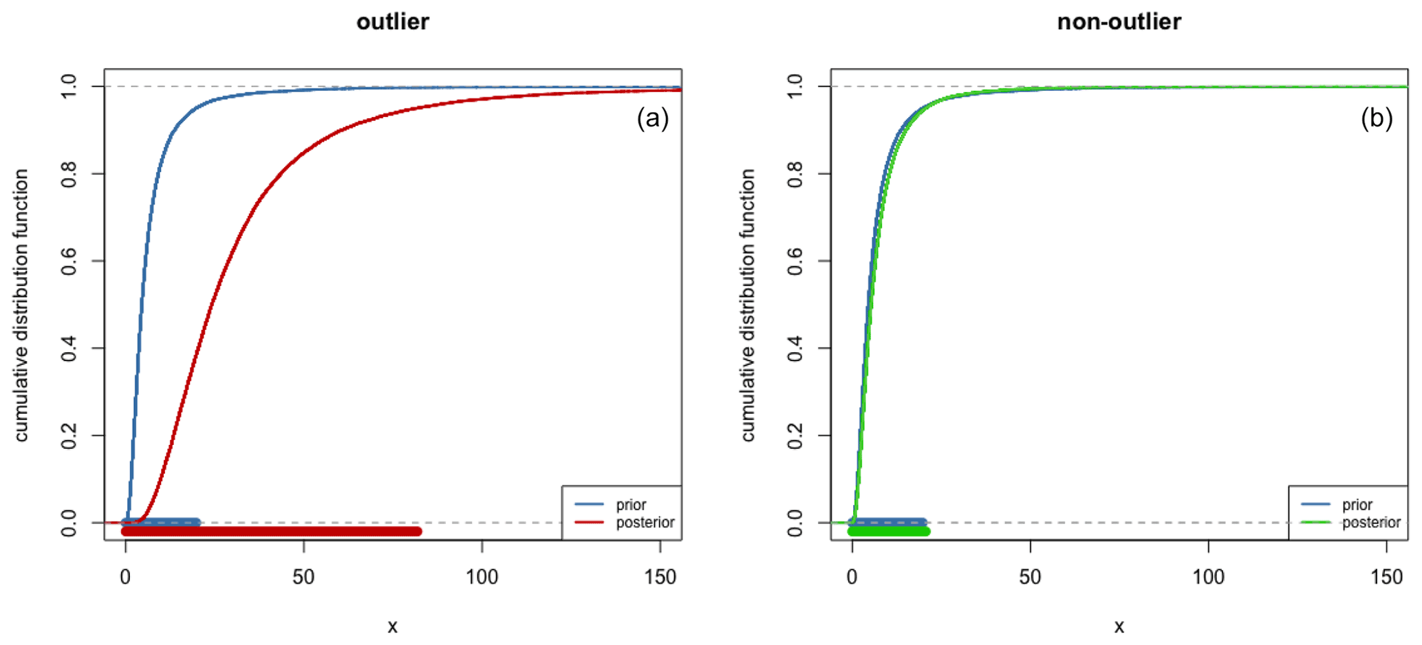
Figure 1Comparison of prior and posterior cumulative distribution functions of individual variance and their 95 % credible interval (bottom horizontal lines): the corresponding equivalent dose is detected as an outlier (a) or not (b).
In this additional step, we adapt the BCAM in including individual random effects. This is the same principle as applied in the event model introduced by Lanos and Philippe (2017, 2018). It amounts to the assumption that the errors have individual variances independently and identically distributed from the same shrinkage distribution as previously chosen for the BCAM. While the event model can be used to estimate A, it suffers from a lack of precision due to the summation of individual variances. Thus, in our approach, we use the posterior distribution of individual variances for constructing a decision rule to detect outliers. Indeed, these parameters measure the dispersion of individual ages around the central age. Therefore, if an equivalent dose is detected as an outlier, its corresponding individual age will take large values with respect to the prior information on . Thus, a De value is identified as an outlier if the posterior distribution of its individual variance is stochastically greater than its prior distribution. To do that, we use quantiles and compare the prior and posterior distributions. More precisely, we fix a probability 1−α close to 1 (for instance, ): if the posterior (1−α) quantile is greater than the prior (1−α) quantile, the associated De is tagged as an outlier and removed from the De distribution (Fig. 1).
When this selection is completed, the age A is estimated with BCAM from the De distribution with the outliers removed, while the posterior distributions are approximated from Markov chain Monte Carlo (MCMC) samples. In practice, we use the Gibbs sampler JAGS (Plummer, 2003) through the associated R (R Core Team, 2021) package “rjags” (Plummer, 2019).
2.2.3 Original data and structure of the model
Input data for the model are values from the and De distributions. The De distribution is a series of central values with associated errors, whereas the distribution represents the probability of each dose-rate value. Additionally, the internal overdispersion (int_OD) obtained from the DRT experiment is required. This parameter is used to modify the Dr distribution to be the same shape as the expected De distribution.
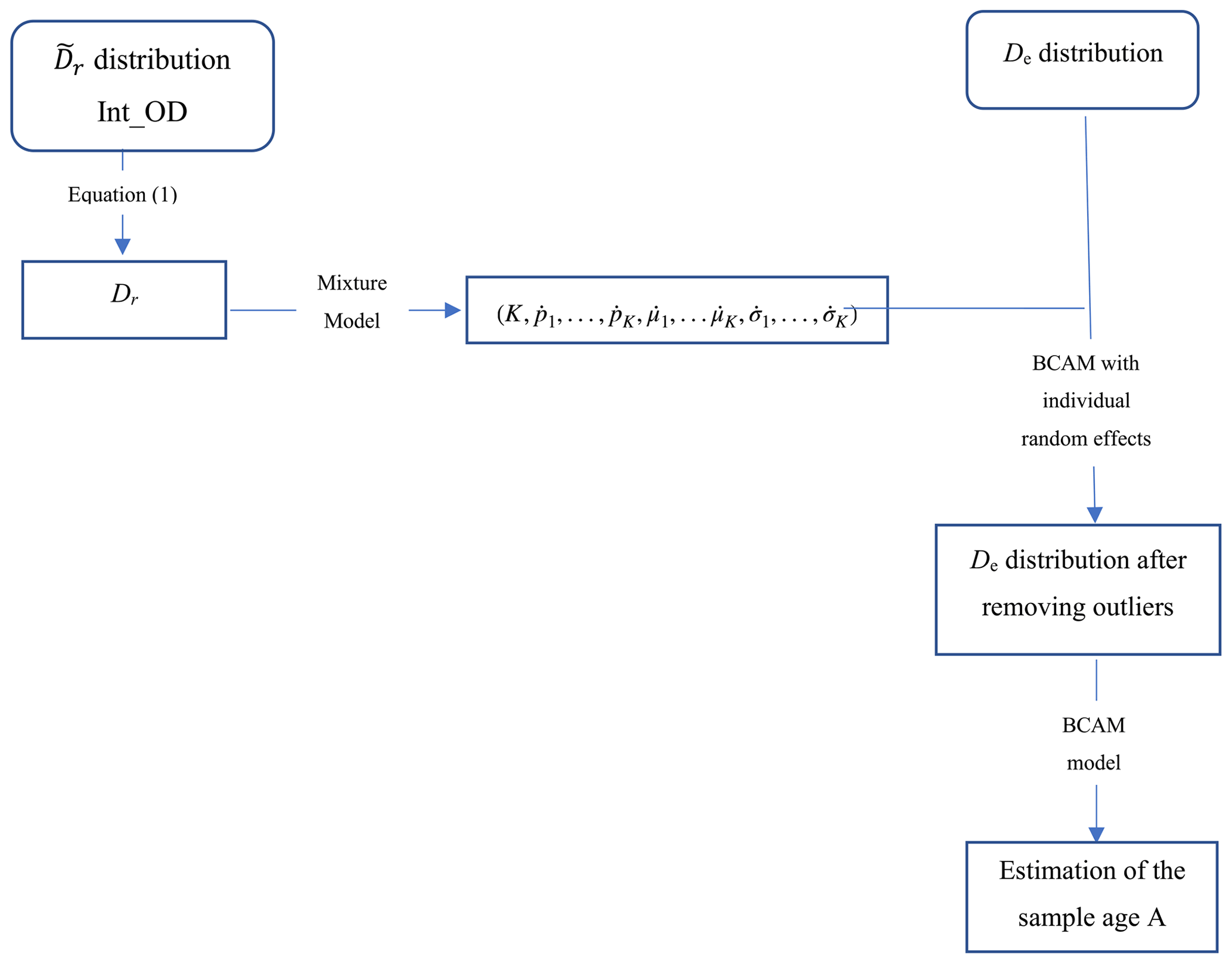
In summary (Fig. 2), the mathematical model to combine the De and Dr distributions consists of four steps.
-
Each value is transformed according to Eq. (1), considering the int_OD value.
-
The Dr distribution is fitted with a weighted sum of normal (Gaussian) densities. The number of functions and their height and width are automatically adjusted to maximize the likelihood function (Fig. 3).
-
After a rough estimation of the individual ages (corresponding to the De values divided by the mean dose rate), the “distance” of each De value and its uncertainty with the model are computed using an MCMC process and compared to a fixed threshold set to 5 %. De values scoring lower than 95 % are considered outliers (Fig. 4).
-
Finally, De values corresponding to the identified outliers are removed from the De distribution, and the age is computed by the Bayesian central age model from this new De distribution. The cumulative probability distribution of the resulting model is then compared with this new De distribution and the original data (Fig. 5).
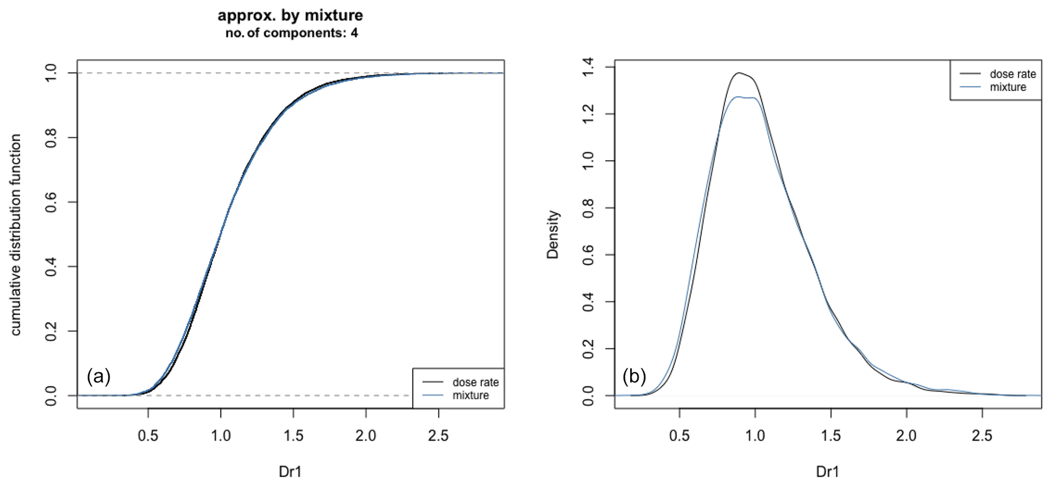

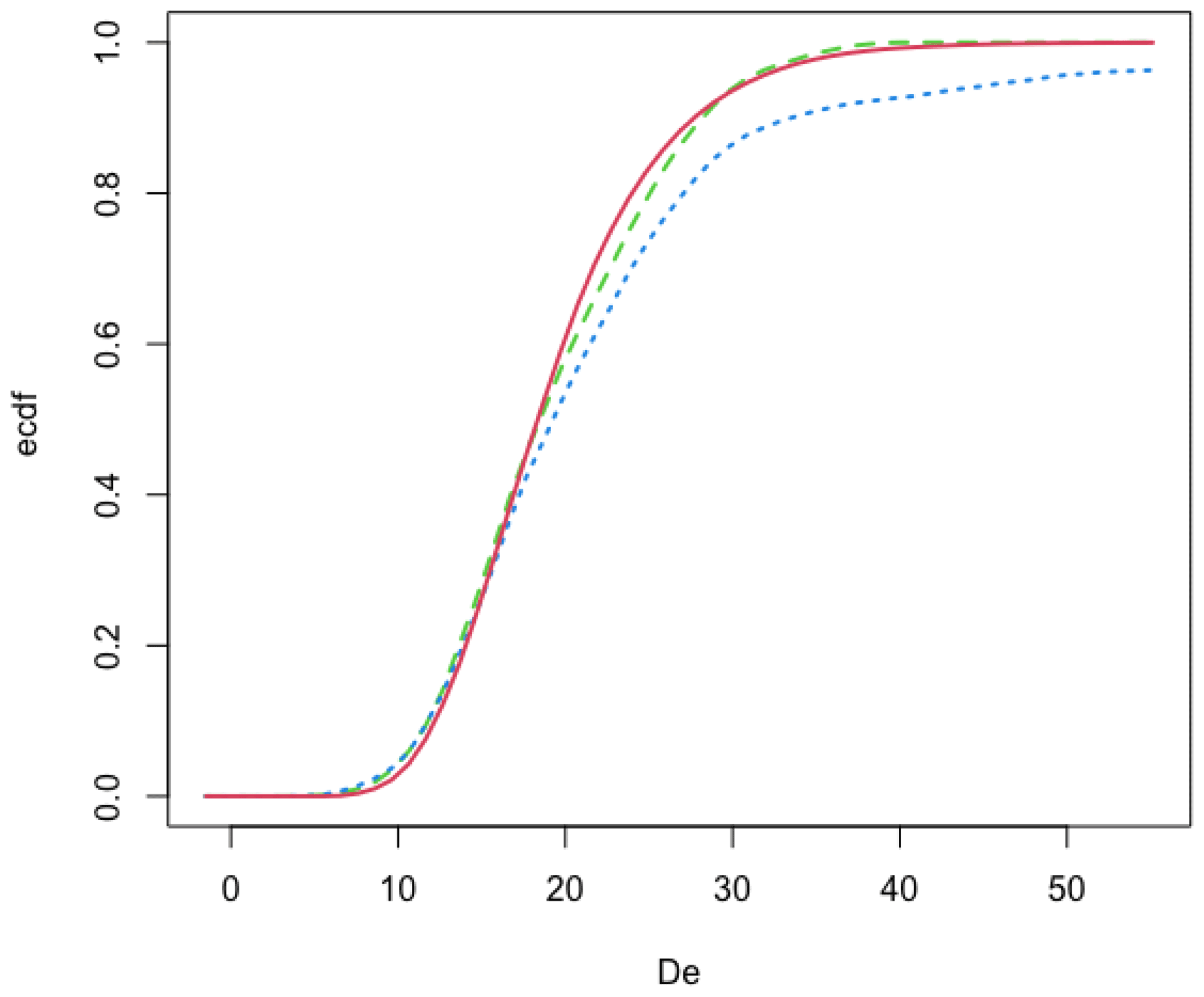
Figure 5Comparison of the cumulative distribution functions: A×Dr (red line), De (dotted blue line), and reduced – after removal of the detected outlier values – De (dashed green line).
2.3 The implementation of BCAM in R
The mathematical model was implemented in R and is available in the package
“Luminescence” (Kreutzer et al., 2012) version ≥ 0.9.16
(Kreutzer et al., 2022) under the function name combine_De_Dr(). The De and Dr distributions can be imported
directly from an Excel™ spreadsheet or CSV file or simply passed as a data.frame (a data object in R, comparable to a spreadsheet) imported through other formats. The other values are directly passed to the function as parameters.
The function combine_De_Dr() returns four plots (Figs. S2–S3 in the Supplement): the first two figures are related to detecting outliers and illustrate the variation of the individual standard deviation of the posterior age distributions. The last two figures show a kernel density plot of the posterior ages and the empirical cumulative distribution function plot. This last figure compares the cumulative De distributions (with or without the identified outliers) with the modelled De distribution (A×Dr). We provide a simple example with R code in the Supplement.
Our tests rely on simulated numerical data (Supplement S2). Complex Dr distributions were built with a series of values (at least 1000 per series) randomly sampled from normal and/or log-normal distributions. From each obtained Dr distribution, 100 values were randomly drawn and multiplied by 50 to represent individual De values (the Dr values vary around 1 Gy ka−1, and the De values are then around 50 and expressed in Gy). Each De value was then associated with an uncertainty randomly sampled from a normal distribution of relative uncertainties N(0.1,0.05).
In cases in which outliers were added to the initial De distribution, their values were randomly determined from a normal or log-normal distribution, and uncertainties were defined as mentioned in the previous paragraph.
3.1 Tests without outliers
Table 1 lists the results of tests performed using four different Dr distributions: (1) a single normal distribution, (2) a sum of two normal distributions, (3) a single log-normal distribution, and (4) a sum of two log-normal distributions. For each Dr distribution, five runs were computed, and De_Dr ages were calculated using the combine_De_Dr() function. Figure 6 shows an example abanico plot (Dietze et al., 2016) of a De distribution for each type of simulated Dr distribution.
Table 1Results of tests without added outliers. Tests were performed with four different shapes of Dr distributions: Norm(n, m, SD) and log-Norm(n, m, SD) indicate normal and log-normal distributions, respectively, where (n) is the number of random values, (m) the mean of the distribution, and (SD) the standard deviation. The number of Gaussian components identified by the model when fitting the Dr distribution is given, as is the number of points identified as outliers. Numbers in bold represent average values.
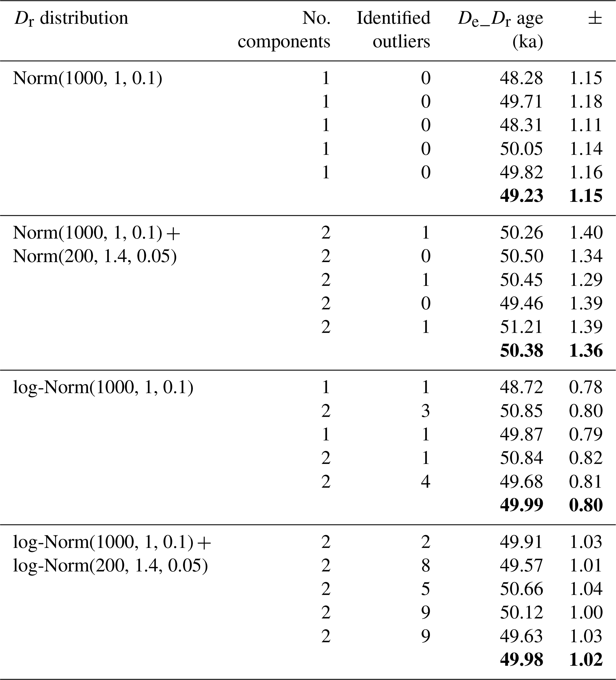
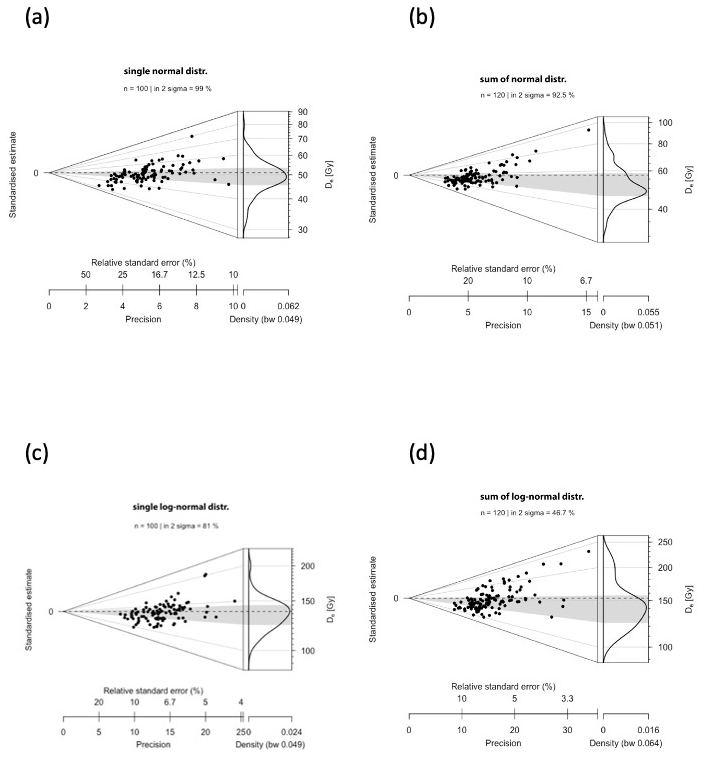
Figure 6Abanico plots of the De distributions (100 values) without outliers. (a) Single normal distribution, (b) sum of two normal distributions, (c) single log-normal distribution, and (d) sum of two log-normal distributions.
For the four distribution types considered in these tests, the De_Dr age is very close to the given age, i.e. 50 ka, demonstrating the efficiency of the De_Dr model. It is also worth mentioning that although we did not add outliers to the initial De distribution, a few values were identified by the model as outliers and were then discarded before the final age was calculated. However, this is not surprising and can be explained by the stochastic nature of the sampling process of the De values, which each had an associated random uncertainty.
3.2 Tests with outliers
Table 2 reports results for De distributions, including 20 outliers in addition to the original 100 values. As indicated in this table, if the initial De values were sampled from a normal distribution, the outlier values were also sampled from a normal distribution (for instance, for , ). Furthermore, when the 100 De values were sampled from a log-normal distribution, the 20 outlier values were also sampled from a log-normal distribution (for instance, for , ).
Table 2Results of tests with 20 outliers added to the original De distribution. Their values were determined following the function indicated in the second column. Notice that the (m) parameter of these functions varied from 1.3 to 1.6, leading to outlier values which, on average, increased, as is observable on the abanico plots (Fig. 7). Numbers in bold represent average values.
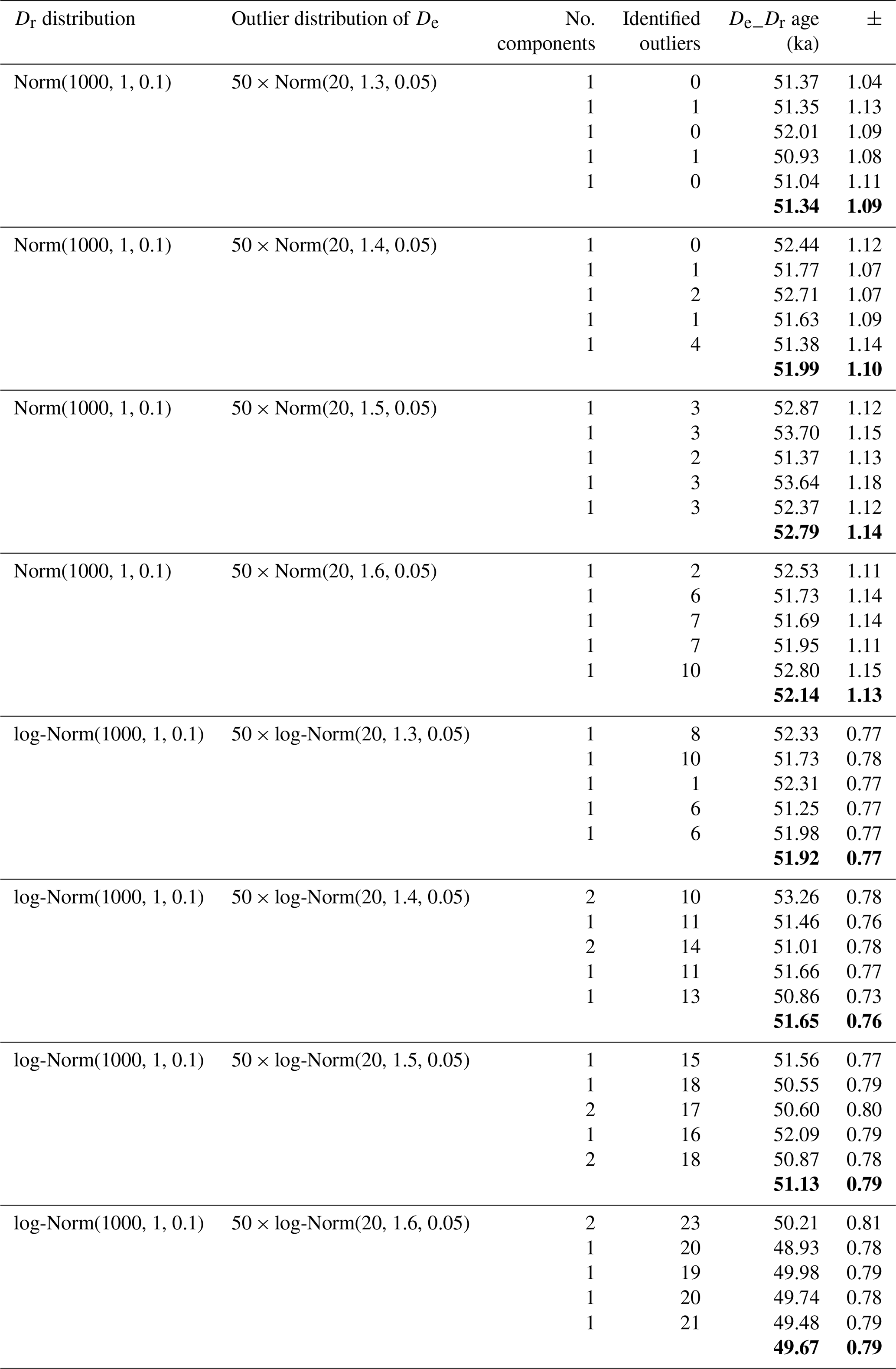
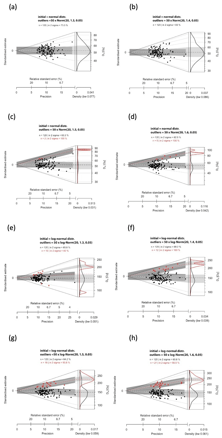
Figure 7Abanico plots of the De distributions (100 initial values sampled from the Dr distribution) to which 20 outlier values have been added: red dots indicate the values identified as outliers (not the values added as outliers). (a–d) Initial De distribution = normal distribution; (e–h) initial De distribution = log-normal distribution. Outlier values (20) added as follows: (a) 50 × Norm(20, 1.3, 0.05); (b) 50 × Norm(20, 1.4, 0.05); (c) 50 × Norm(20, 1.5, 0.05); (d) 50 × Norm(20, 1.6, 0.05) and (e) 50 × log-Norm(20, 1.3, 0.05); (f) 50 × log-Norm(20, 1.4, 0.05); (g) 50 × log-Norm(20, 1.5, 0.05); (h) 50 × log-Norm(20, 1.6, 0.05).
The De_Dr age is slightly higher than 50 ka in all cases because a few outlier values overlap randomly with the initial De distribution and were therefore not identified as outliers by the De_Dr approach. However, this overestimation remains low (< 5 % of the true age), whereas outliers represent almost 17 % () of the De values. Examples are illustrated in Fig. 7 as abanico plots (Dietze et al., 2016).
Table 3For each type of Dr distribution (normal or log-normal), outlier values were added following either the function 50 × Norm(n, 1.3, 0.05) or the function 50 × log-Norm(n, 1.3, 0.05). The number of outliers (n) varied from 0 to 50 (then representing between 0 % and 33 % of the initial De distribution). The age error is the 95 % credible interval.
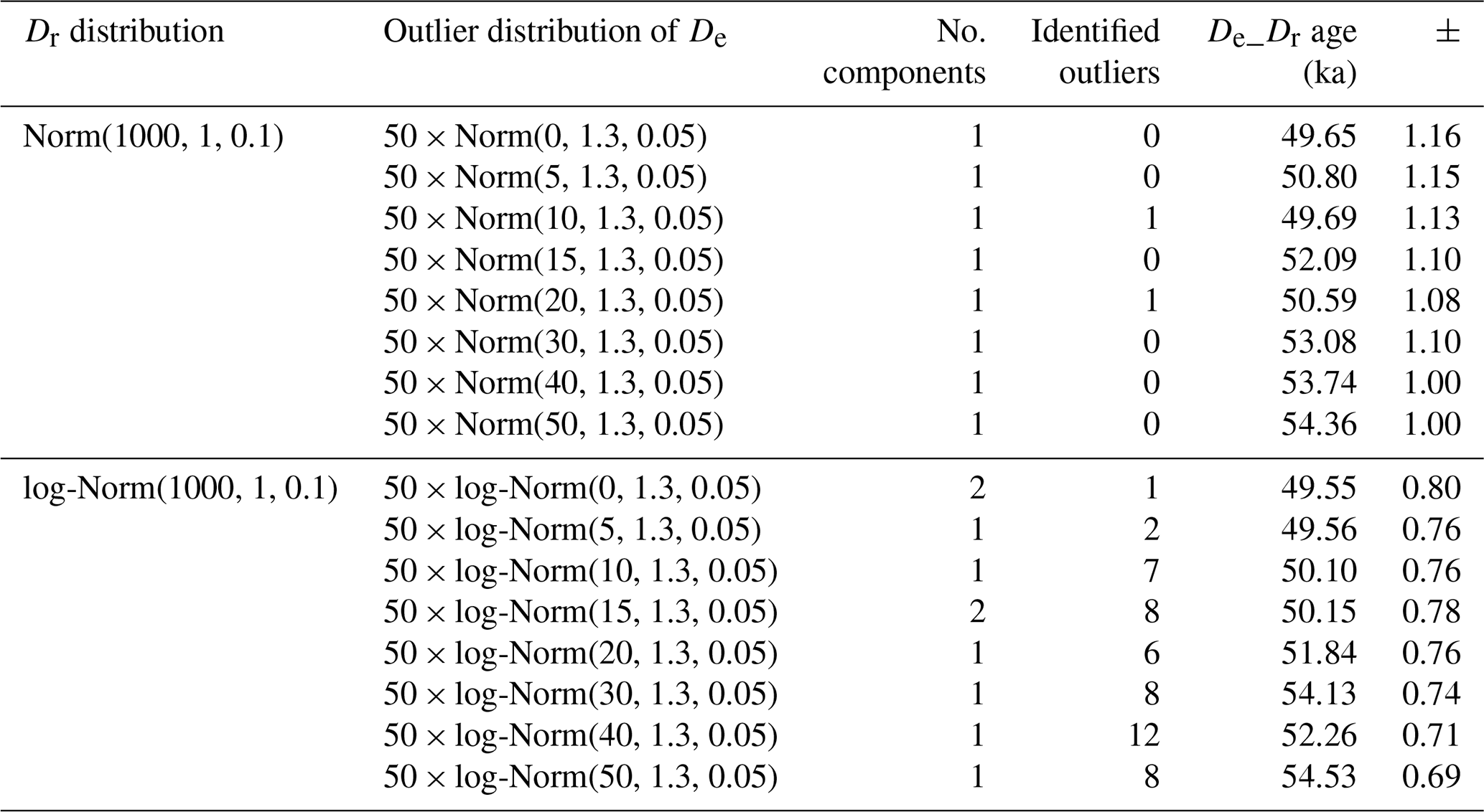

Figure 8De_Dr age as a function of the number of outliers added to the initial De distribution (the expected age is 50 ka, indicated by the red line). Norm and log-Norm represent the functions from which the initial De distributions (comprising 100 values) were built. Error bars represent 95 % credible intervals. Dotted lines are ±10 %.
To test the model's performance to identify outliers when their values are close to the initial De values, we simulated normal and log-normal distributions with outliers that followed our setting from above: for , and for , , where this time n varied from 0 to 50 (then representing between 0 % and 33 % of the initial De distribution). The results are given in Table 3 and displayed in Fig. 8. The De_Dr ages increase with the percentage of outliers, but the overestimation remains below 10 % of the true age in all cases. This result is particularly interesting because these simulations represent cases in which a series of poorly bleached grains (i.e. the outliers) whose De values are not significantly different from the mean De have been measured in addition to well-bleached grains (initial De values).
Results show that the De_Dr model works well for De distributions without outliers. It also gives satisfactory results when the De values of the outliers are significantly different from the individual De values composing the target population. On the other hand, the existence of values defined as outliers but very close to the target population may be assimilated by the model to the target population and thus not be identified as outliers. This is related to the fact that the De_Dr model is a “majority rule” model.
This notion of majority is vital because it sets the limits of the model's applicability. If the number of outliers is significantly larger than the number of De values representing the target population, the De_Dr model will combine the De and Dr distributions as best as possible so that a maximum of De values corresponds to (A×Dr) values. A visual examination of the distributions calculated by the model (e.g. Fig. 5) is therefore indispensable, as is a visual examination of the outliers identified within the distribution of individual ages (e.g. Fig. 4).
On the plus side, it is also important to recall that the De_Dr model does not require a pre-defined function to represent the De distribution. For the tests carried out previously, the type of distribution (normal, log-normal, or a mixture of those distributions) was fixed to randomly draw the simulated values only. However, the type of chosen distribution and the parameters characterizing it (mean and variance) were not supplied to the model. In other words, the De_Dr model did not know about those parameters.
Nevertheless, the De_Dr model does require a precise determination of the Dr distribution. To date, this distribution can be obtained either from numerical sediment models considering bulk density, grain size composition, mineralogy and the spatial distribution of radio-elements (for a possible 2D approach, see Dietze et al., 2021), or it can be obtained experimentally using nuclear detectors (e.g. Romanyukha et al., 2017; Fu et al., 2022). Unfortunately, at present, such experiments are scarce and remain relatively difficult to implement. Supposing they become more common, systematic comparisons between the De_Dr model, which provides the most probable age, and other models leading to the De value most representative of the event to be dated will become possible in a future contribution. Moreover, perhaps cases will be observed in which the Dr distributions do not follow a simple distribution (typically log-normal) as already suggested by Martin et al. (2015b).
One output of the model is the posterior distribution of the A defined
through a simulated Markov chain. The highest posterior density interval
(HPDI), a region of the density curve encompassing a particular credible
interval (e.g. 68 % or 95 %), can be calculated from this distribution. The HPD, the HPDI, the mean, , and the standard deviation, SDA, of the posterior distribution can be calculated with the function Luminescence::plot_OSLAgeSummary() (see Supplement S1). If the posterior distribution of the age is a Gaussian distribution, the HPDI coincides with the interval at a 68 % credible level ( at 95 %). The lower and upper end of the
value of the HPDI can be supplemented to facilitate systematic errors
associated with the average total dose rate and the source dose rate of the
equipment used for the De measurements. Two approaches are feasible. (1) The typical approach consists of modifying the precision, with the standard deviation SDA being replaced by , where p denotes the relative error (in %) associated with the systematic error. (2) To preserve the HPD region that
considers the possible asymmetry of the posterior distribution, the
systematic error can be modelled by , where
ϵ is a standard Gaussian variable independent of the age. One
can then easily sample from the corrected age and update the HPD region. If
the probability distribution of is a Gaussian distribution, the two
approaches are equivalent.
To date, the De_Dr model is thus the first model that allows considering the information from the equivalent doses and dose rates simultaneously, thus offering a substantial paradigm change compared to existing approaches.
The De_Dr model is an alternative to statistical models to determine the target population from a De distribution. Combining the information associated with the equivalent doses and dose rates experienced by the grains during burial, the model offers the possibility to determine the age of the target population without any pre-defined function representing the De distribution.
Future work should focus on tests carried out on well-dated samples (typically cross-checked with 14C dating) to validate the De_Dr model experimentally. This would, however, first necessitate access to accurately and precisely determined Dr distributions.
The source code of the model is part of the R package “Luminescence” (≥ v0.9.16) and available open-access under GPL-3 licence conditions (https://CRAN.R-project.org/package=Luminescence, last access: 8 September 2021; https://doi.org/10.5281/zenodo.6345291, Kreutzer et al., 2022).
The supplement related to this article is available online at: https://doi.org/10.5194/gchron-4-297-2022-supplement.
NM and CT initiated the work by writing the first paper draft and an initial R script. JMG and AP developed the mathematical basis for the model. SK implemented the model in the R package “Luminescence” and ran additional tests. All authors equally contributed to the discussion and the final paper write-up.
The contact author has declared that neither they nor their co-authors have any competing interests.
Publisher's note: Copernicus Publications remains neutral with regard to jurisdictional claims in published maps and institutional affiliations.
Sebastian Kreutzer is grateful to the European Union for providing a Marie Skłodowska-Curie grant.
This research has been supported by the Agence Nationale de la Recherche (grant no. ANR-10-LABX-52) and the European Union's Horizon 2020 research and innovation programme (CREDit, grant no. 844457).
This paper was edited by Julie Durcan and reviewed by Alastair Cunningham and one anonymous referee.
Cunningham, A. C. and Wallinga, J.: Realizing the potential of fluvial archives using robust OSL chronologies, Quat. Geochronol., 12, 98–106, https://doi.org/10.1016/j.quageo.2012.05.007, 2012.
Cunningham, A. C., DeVries, D. J., and Schaart, D. R.: Experimental and computational simulation of beta-dose heterogeneity in sediment, Radiat. Meas., 47, 1060–1067, https://doi.org/10.1016/j.radmeas.2012.08.009, 2012.
Cunningham, A. C., Wallinga, J., Hobo, N., Versendaal, A. J., Makaske, B., and Middelkoop, H.: Re-evaluating luminescence burial doses and bleaching of fluvial deposits using Bayesian computational statistics, Earth Surf. Dynam., 3, 55–65, https://doi.org/10.5194/esurf-3-55-2015, 2015.
Dempster, A. P., Laird, N. M., and Rubin, D. B.: Maximum Likelihood from Incomplete Data Via the EM Algorithm, J. R. Stat. Soc. Ser. B Methodol., 39, 1–22, https://doi.org/10.1111/j.2517-6161.1977.tb01600.x, 1977.
Dietze, M., Kreutzer, S., Burow, C., Fuchs, M. C., Fischer, M., and Schmidt, C.: The abanico plot: visualising chronometric data with individual standard errors, Quat. Geochronol., 31, 12–18, https://doi.org/10.1016/j.quageo.2015.09.003, 2016.
Dietze, M., Kreutzer, S., Fuchs, M. C., and Meszner, S.: sandbox – Creating and Analysing Synthetic Sediment Sections with R, Geochronology Discuss. [preprint], https://doi.org/10.5194/gchron-2021-39, in review, 2021.
Duller, G. A. T., Bøtter-Jensen, L., Murray, A. S., and Truscott, A. J.: Single grain laser luminescence (SGLL) measurements using a novel automated reader, Nucl. Instrum. Meth. B, 155, 506–514, https://doi.org/10.1016/S0168-583X(99)00488-7, 1999a.
Duller, G. A. T., Bøtter-Jensen, L., Kohsiek, P., and Murray, A. S.: A High-Sensitivity Optically Stimulated Luminescence Scanning System for Measurement of Single Sand-Sized Grains, Radiat. Prot. Dosimetry, 84, 325–330, https://doi.org/10.1093/oxfordjournals.rpd.a032748, 1999b.
Fang, F., Martin, L., Williams, I. S., Brink, F., Mercier, N., and Grün, R.: 2D modelling: A Monte Carlo approach for assessing heterogeneous beta dose rates in luminescence and ESR dating: Paper II, application to igneous rocks, Quat. Geochronol., 48, 195–206, https://doi.org/10.1016/j.quageo.2018.07.005, 2018.
Fu, X., Romanyukha, A. A., Li, B., Jankowski, N. R., Lachlan, T. J., Jacobs, Z., George, S. P., Rosenfeld, A. B., and Roberts, R. G.: Beta dose heterogeneity in sediment samples measured using a Timepix pixelated detector and its implications for optical dating of individual mineral grains, Quat. Geochronol., 68, 101254, https://doi.org/10.1016/j.quageo.2022.101254, 2022.
Fuchs, M. and Lang, A.: OSL dating of coarse-grain fluvial quartz using single-aliquot protocols on sediments from NE Peloponnese, Greece, Quaternary Sci. Rev., 20, 783–787, https://doi.org/10.1016/S0277-3791(00)00040-8, 2001.
Galbraith, R. F., Roberts, R. G., Laslett, G. M., Yoshida, H., and Olley, J. M.: Optical dating of single and multiple grains of Quartz from Jinmium Rock Shelter, Northern Australia: Part I, Experimental design and statistical models, Archaeometry, 41, 339–364, https://doi.org/10.1111/j.1475-4754.1999.tb00987.x, 1999.
Galharret, J.-M., Philippe, A., and Mercier, N.: Detection of outliers with a Bayesian hierarchical model: application to the single-grain luminescence dating method, Electron. J. Appl. Stat. Anal., North America, 14, 318–338, http://siba-ese.unisalento.it/index.php/ejasa/article/view/22661, last access: 26 October 2021.
Guérin, G., Jain, M., Thomsen, K. J., Murray, A. S., and Mercier, N.: Modelling dose rate to single grains of quartz in well-sorted sand samples: The dispersion arising from the presence of potassium feldspars and implications for single grain OSL dating, Quat. Geochronol., 27, 52–65, https://doi.org/10.1016/j.quageo.2014.12.006, 2015.
Guérin, G., Christophe, C., Philippe, A., Murray, A. S., Thomsen, K. J., Tribolo, C., Urbanova, P., Jain, M., Guibert, P., Mercier, N., Kreutzer, S., and Lahaye, C.: Absorbed dose, equivalent dose, measured dose rates, and implications for OSL age estimates: Introducing the Average Dose Model, Quat. Geochronol., 41, 163–173, https://doi.org/10.1016/j.quageo.2017.04.002, 2017.
Guibert, P., Christophe, C., Urbanova, P., Guérin, G., and Blain, S.: Modeling incomplete and heterogeneous bleaching of mobile grains partially exposed to the light_Towards a new tool for single grain OSL dating of poorly bleached mortars, Radiat. Meas., 107, 48–57, https://doi.org/10.1016/j.radmeas.2017.10.003, 2017.
Kalchgruber, R., Fuchs, M., Murray, A. S., and Wagner, G. A.: Evaluating dose-rate distributions in natural sediments using α-Al2O3:C grains, Radiat. Meas., 37, 293–297, https://doi.org/10.1016/S1350-4487(03)00012-X, 2003.
Kreutzer, S., Schmidt, C., Fuchs, M. C., Dietze, M., Fischer, M., and Fuchs, M.: Introducing an R package for luminescence dating analysis, Anc. TL, 30, 1–8, http://ancienttl.org/ATL_30-1_2012/ATL_30-1_Kreutzer_p1-8.pdf (last access: 8 September 2021), 2012.
Kreutzer, S., Burow, C., Dietze, M., Fuchs, M. C., Schmidt, C., Fischer, M., Friedrich, J., Mercier, N., Smedley, R. K., Christophe, C., Zink, A., Durcan, J., King, G. E., Philippe, A., Guérin, G., Riedesel, S., Autzen, M., Guibert, P., Mittelstrass, D., Gray, H. J., and Galharret, J.-M.: Luminescence: Comprehensive Luminescence Dating Data Analysis (0.9.19), Zenodo [code], https://doi.org/10.5281/zenodo.6345291, 2022.
Lanos, P. and Philippe, A.: Hierarchical Bayesian modeling for combining dates in archeological context, J. Société Fr. Stat., 158, 72–88, 2017.
Lanos, P. and Philippe, A.: Event date model: a robust Bayesian tool for chronology building, Commun. Stat. Appl. Methods, 25, 131–157, https://doi.org/10.29220/csam.2018.25.2.131, 2018.
Lepper, K. and McKeever, S. W. S.: An objective methodology for dose distribution analysis, Radiat. Prot. Dosimetry, 101, 349–252, https://doi.org/10.1093/oxfordjournals.rpd.a005999, 2002.
Li, B., Jacobs, Z., and Roberts, R. G.: Bayesian analysis of De distributions in optical dating: Towards a robust method for dealing with outliers, Quat. Geochronol., 67, 101230, https://doi.org/10.1016/j.quageo.2021.101230, 2021.
Martin, L., Incerti, S., and Mercier, N.: DosiVox: Implementing Geant 4-based software for dosimetry simulations relevant to luminescence and ESR dating techniques, Anc. TL, 33, 1–10, http://ancienttl.org/ATL_33-1_2015/ATL_33-1_Martin_p1-10.pdf (last access: 8 September 2021), 2015a.
Martin, L., Mercier, N., Incerti, S., Lefrais, Y., Pecheyran, C., Guérin, G., Jarry, M., Bruxelles, L., Bon, F., and Pallier, C.: Dosimetric study of sediments at the Beta dose rate scale: characterization and modelization with the DosiVox software, Radiat. Meas., 81, 134–141, https://doi.org/10.1016/j.radmeas.2015.02.008, 2015b.
Martin, L., Fang, F., Mercier, N., Incerti, S., Grün, R., and Lefrais, Y.: 2D modelling: A Monte Carlo approach for assessing heterogeneous beta dose rate in luminescence and ESR dating: Paper I, theory and verification, Quat. Geochronol., 48, 25–37, https://doi.org/10.1016/j.quageo.2018.07.004, 2018.
Mayya, Y. S., Morthekai, P., Murari, M. K., and Singhvi, A. K.: Towards quantifying beta microdosimetric effects in single-grain quartz dose distribution, Radiat. Meas., 41, 1032–1039, https://doi.org/10.1016/j.radmeas.2006.08.004, 2006.
Nathan, R. P., Thomas, P. J., Jain, M., Murray, A. S., and Rhodes, E. J.: Environmental dose rate heterogeneity of beta radiation and its implications for luminescence dating: Monte Carlo modelling and experimental validation, Radiat. Meas., 37, 305–313, https://doi.org/10.1016/s1350-4487(03)00008-8, 2003.
Plummer, M.: JAGS: A program for analysis of Bayesian graphical models using Gibbs sampling, 3rd International Workshop on Distributed Statistical Computing (DSC 2003), 20–22 March 2003, Vienna, Austria, DSC Work. Pap., 124, 1–10, 2003.
Plummer, M.: rjags: Bayesian Graphical Models using MCMC, R package version 4-10, https://CRAN.R-project.org/package=rjags (last access: 8 September 2021), 2019.
R Core Team: R: A Language and Environment for Statistical Computing, R Foundation for Statistical Computing, Vienna, Austria, https://www.r-project.org, last access: 8 September 2021.
Roberts, R. G., Galbraith, R. F., Yoshida, H., Laslett, G. M., and Olley, J. M.: Distinguishing dose populations in sediment mixtures: a test of single-grain optical dating procedures using mixtures of laboratory-dosed quartz, Radiat. Meas., 32, 459–465, https://doi.org/10.1016/S1350-4487(00)00104-9, 2000.
Romanyukha, A. A., Cunningham, A. C., George, S. P., Guatelli, S., Petasecca, M., Rosenfeld, A. B., and Roberts, R. G.: Deriving spatially resolved beta dose rates in sediment using the Timepix pixelated detector, Radiat. Meas., 106, 483–490, https://doi.org/10.1016/j.radmeas.2017.04.007, 2017.
Rufer, D. and Preusser, F.: Potential of Autoradiography to Detect Spatially Resolved Radiation Patterns in the Context of Trapped Charge Dating, Geochronometria, 34, 1–13, https://doi.org/10.2478/v10003-009-0014-4, 2010.
Scrucca, L., Fop, M., Murphy, T. B., and Raftery, A. E.: mclust 5: Clustering, Classification and Density Estimation Using Gaussian Finite Mixture Models, R J., 8, 289–317, https://doi.org/10.32614/RJ-2016-021, 2016.
Spiegelhalter, D. J., Abrams, K. R., and Myles, J. P.: Bayesian approaches to clinical trials and health-care evaluation, Wiley, Chichester, ISBN 978-0-470-09259-0, 2004.
Thomsen, K. J., Murray, A. S., Bøtter-Jensen, L., and Kinahan, J.: Determination of burial dose in incompletely bleached fluvial samples using single grains of quartz, Radiat. Meas., 42, 370–379, https://doi.org/10.1016/j.radmeas.2007.01.041, 2007.
Woda, C. and Fuchs, M.: On the applicability of the leading edge method to obtain equivalent doses in OSL dating and dosimetry, Radiat. Meas., 43, 26–37, https://doi.org/10.1016/j.radmeas.2007.12.006, 2008.