the Creative Commons Attribution 4.0 License.
the Creative Commons Attribution 4.0 License.
 | 08 Nov 2022
Cosmogenic 3He paleothermometry on post-LGM glacial bedrock within the central European Alps
Natacha Gribenski
Marissa M. Tremblay
Pierre G. Valla
Greg Balco
Benny Guralnik
David L. Shuster
Diffusion properties of cosmogenic 3He in quartz at Earth surface temperatures offer the potential to directly reconstruct the evolution of past in situ temperatures from formerly glaciated areas, which is important information for improving our understanding of glacier–climate interactions. In this study, we apply cosmogenic 3He paleothermometry to rock surfaces gradually exposed from the Last Glacial Maximum (LGM) to the Holocene period along two deglaciation profiles in the European Alps (Mont Blanc and Aar massifs). Laboratory experiments conducted on one representative sample per site indicate significant differences in 3He diffusion kinetics between the two sites, with quasi-linear Arrhenius behavior observed in quartz from the Mont Blanc site and complex Arrhenius behavior observed in quartz from the Aar site, which we interpret to indicate the presence of multiple diffusion domains (MDD). Assuming the same diffusion kinetics apply to all quartz samples along each profile, forward model simulations indicate that the cosmogenic 3He abundance in all the investigated samples should be at equilibrium with present-day temperature conditions. However, measured cosmogenic 3He concentrations in samples exposed since before the Holocene indicate an apparent 3He thermal signal significantly colder than today. This observed 3He thermal signal cannot be explained with a realistic post-LGM mean annual temperature evolution in the European Alps at the study sites. One hypothesis is that the diffusion kinetics and MDD model applied may not provide sufficiently accurate, quantitative paleo-temperature estimates in these samples; thus, while a pre-Holocene 3He thermal signal is indeed preserved in the quartz, the helium diffusivity would be lower at Alpine surface temperatures than our diffusion models predict. Alternatively, if the modeled helium diffusion kinetics is accurate, the observed 3He abundances may reflect a complex geomorphic and/or paleoclimatic evolution, with much more recent ground temperature changes associated with the degradation of alpine permafrost.
- Article
(7846 KB) - Full-text XML
-
Supplement
(4020 KB) - BibTeX
- EndNote


This study applies cosmogenic noble gas paleothermometry (Tremblay et al., 2014a) to attempt to reconstruct temperature changes associated with gradual ice lowering following the Last Glacial Maximum (LGM, ca. 27–19 ka; Clark et al., 2009) in two sites of the high European Alps. Because glaciers are sensitive to both temperature and precipitation, obtaining information about in situ temperature conditions from an independent proxy is critical to disentangling the role of either variable in recorded glacier fluctuations and to adequately use these records for paleoclimate reconstructions. In particular, paleoglacier records can be used as direct, site-specific paleo-precipitation indicators (e.g., Kerschner et al., 2000; Kerschner and Ivy-Ochs, 2008; Martin et al., 2020) to trace changes in regional atmospheric circulation systems (Kuhlemann et al., 2008; Becker et al., 2016; Gribenski et al., 2021). More detailed information about paleoclimate conditions would moreover improve both our understanding of glacier responses to current climate change as well as our ability to anticipate glacier evolutions for proposed future climate scenarios (Zemp et al., 2006; Haeberli et al., 2022). Furthermore, direct temperature constraints associated with paleoglacier variations are also critical to our understanding of glacier erosion processes (Hallet, 1979), which have profoundly shaped high-latitude and mountain landscapes over 103 to 106-year timescales (Herman et al., 2021) and which seem to relate to climatic conditions, among other factors (Koppes et al., 2015; Cook et al., 2020).
Available data on the relationship between glacier geometry and climate, as well as between glacial erosion and climate, are largely biased toward present-day and historical time periods, therefore obliging us to rely on the assumption that modern to centennial records are representative of the range of variation and mechanistic trends between climate–glacier variation and erosion operating on geological time scales (Jaeger and Koppes, 2016). While combined records of paleoglacier geometry and erosion rates on Late Pleistocene timescales are growing due to the recent development of analytical and numerical techniques (e.g., Kapannusch et al., 2020; Mariotti et al., 2021), obtaining direct quantitative paleoclimate constraints from formerly glaciated areas remains challenging, even for regions with relatively well-known paleoglacial histories. In the European Alps, the most detailed paleoglacier record goes back to the Late Pleistocene ice maximum advance, dated around ∼ 26–24 ka in the northern and central Alps (Monegato et al., 2017), in line with the global LGM. During the LGM, ice spread to within several tens of kilometers of the piedmonts and reached more than 1000–1500 m thickness in the main valleys (Ivy-Ochs, 2015; Wirsig et al., 2016a; Serra et al., 2022). More restricted stages (i.e., Gschnitz, Daun, Egesen stadials; Ivy-Ochs, 2015) marking the gradual retreat (and thinning) of the ice into the upper catchments followed between the LGM and the Younger Dryas cooling event (YD, 12.8–11.7 ka; Heiri et al., 2014a). During the early Holocene (i.e., the last 11 ka; Heiri et al., 2014a), glaciers retreated quickly behind the position where the Little Ice Age moraines are located today and remained within these limits for the rest of the Holocene period (Heiri et al., 2014a).
The timing and pattern of paleoglacier variations in the European Alps are consistent with polar ice oxygen isotope (δ18O) records from the Northern Hemisphere (North Greenland Ice Core Project members, 2004), which indicate that maximum Greenland temperature anomalies of around −20 ∘C were reached at 25–20 ka, followed by a gradual warming until ca. 10 ka, with the last pronounced isotopic excursion marked by a −15 ∘C temperature anomaly occurring at ca. 12 ka in association with the YD event (Buizert et al., 2018). After the YD, temperatures stabilized around values similar to today, with only minor fluctuations (less than 2 ∘C) throughout the remaining Holocene period (Buizert et al., 2018). High-resolution δ18O in Alpine speleothems similarly support a coupling between the northern European Alps and Greenland records (Moseley et al., 2020; Li et al., 2021).
While there is evidence for a temporal coupling, a direct, scaled translation of polar ice records over the Alps to obtain quantitative temperature and precipitation constraints is not valid. Indeed, major climate forcing components, such as ice sheet extent, atmospheric greenhouse gas concentrations, and changes in ocean circulation, also underwent large-scale changes between the LGM and the Holocene transition (Clark et al., 2012). This resulted in variable atmospheric circulation patterns (Eynaud et al., 2009) and variable latitudinal temperature gradients (Heiri et al., 2014b) in the Northern Hemisphere during this period. Existing past climate information from Alpine paleoenvironmental proxies is mainly qualitative, with only a few scarce and fragmented quantitative temperature and precipitation records available for the pre-Holocene period (Heiri et al., 2014a). These are mostly from pollen and chironomid proxy records located on the outer rim of the Alpine range from lake and peat archives (Heiri et al., 2014a), noble gas proxy records from groundwater and speleothems (Beyerle et al., 1998; Ghadiri et al., 2018), and tentative inverse glacial modeling (Kerschner and Ivy-Ochs, 2008; Becker et al., 2016; Seguinot et al., 2018), with some noticeable variability in derived paleoclimate information between and within proxy records. Proposed reconstructed mean temperature anomalies during the LGM hence vary from −11 to −14 ∘C based on pollen reconstructions (Wu et al., 2007; Bartlein et al., 2011), −5 to −9 ∘C based on noble gas groundwater records (Beyerle et al., 1998, Seltzer et al., 2021), and −8 to −15 ∘C using glacial modeling studies calibrated on reconstructed ice limits and estimates of paleo-equilibrium line altitude (ELA; i.e., the elevation at which the annual net ice budget in a glacier equals zero; Allen et al., 2008; Becker et al., 2016; Seguinot et al., 2018; Višnjević et al., 2020). LGM precipitation conditions are even more uncertain, with estimates for precipitation anomalies varying widely between −20 % and −60 % (e.g., Peyron et al., 1998; Luetscher et al., 2015; Becker et al., 2016) and for which a differential north–south distribution pattern (Florineth and Schlüchter, 2000; Luetscher et al., 2015; Becker at al., 2016) is still debated (Seguinot et al., 2018; Višnjević et al., 2020). Similarly, little is known regarding climatic conditions during the Late Glacial period between the LGM and the YD; besides that, significantly lower summer temperatures (> 6 ∘C negative anomalies) were still persisting before ca. 15 ka based on chironomid and treeline proxies (Heiri et al., 2014a). During the short-lived (∼ 1 kyr) YD cooling event, temperatures dropped, with mean annual anomalies varying between 2–3 and 5–9 ∘C below present-day values, depending on the considered proxy between paleoglacial reconstructions (e.g., Protin et al., 2019; Baroni et al., 2021), lacustrine pollen assemblages (Magny et al., 2001), and noble gas speleothem records (Ghadiri et al., 2018; Affolter et al., 2019). On the other hand, for the Holocene period, all the available records are in general agreement, indicating that temperature conditions relatively similar to today prevailed, with only minor (less than 2 ∘C) deviations (e.g., Davis et al., 2003; Heiri et al., 2014a; Ghadiri et al., 2018; Affolter et al., 2019).
There is a crucial lack of direct and quantitative in situ temperature constraints from within the Alpine massifs during the different reconstructed glacial stages since the LGM. In this study, we attempt to reconstruct paleotemperatures in the high Alps during the Late Glacial period by applying cosmogenic noble gas paleothermometry (Tremblay et al., 2014a). This method exploits the diffusive behavior of cosmogenic 3He in quartz minerals at Earth surface temperatures (Brook et al., 1993; Shuster and Farley, 2005). Using forward models of cosmogenic 3He production and thermally activated diffusive loss, quantitative constraints on the thermal history of an exposed rock surface can thus be inferred from the difference between surface-exposure ages derived from the diffusive 3He system and from a cosmogenic nuclide that does not experience diffusive loss (Tremblay et al., 2014a, b, 2018). Cosmogenic 3He paleothermometry provides a unique opportunity to obtain quantitative information about past temperatures from in situ rock surfaces located in the formerly glaciated Alps. Here, we explore the applicability of cosmogenic 3He paleothermometry along two deglaciation profiles in the northern and western Alps. The advantages of such sampling targets are (1) relatively simple exposure history of rock surfaces revealed between the LGM and YD (Wirsig et al., 2016b; Lehmann et al., 2020), with limited shadowing effect (e.g., steep surface, limited vegetation, or postglacial sediment cover), and (2) the access to sequences of gradually exposed but lithologically similar samples, enabling a semi-continuous record of a temperature-change history. Based on 3He analytical measurements and forward model simulations, we aim to investigate the sensitivity of the in situ quartz–3He system in two different high Alpine areas and its suitability for the preservation of a 3He thermal signal on Late Pleistocene timescales. We also compare our results to previous studies applying cosmogenic 3He paleothermometry elsewhere in the Alps to gain a further understanding of 3He diffusion behavior in quartz at Earth surface temperatures.
Two sites located in major Alpine massifs were selected for this study and have been previously investigated for their deglaciation history: the Mont Blanc Trelaporte (MBTP) profile (Mont Blanc massif, France; Lehmann et al., 2020), located in the western Alps along the western flank of the Mer de Glace valley (NNE exposure); and the SW-exposed Gelmersee (GELM) ridge (Aar massif, Switzerland; Wirsig et al., 2016b), formed by a hanging valley on the east wall of the Haslital valley in the northern central Alps (Fig. 1, inset). Both sites have steep valley sides that are several hundred meters high with ∼ 30–35∘ slopes and are characterized by smoothly abraded rock surfaces and “roche moutonnée”-like features molded by flowing glaciers. Homogeneous lithologies are exposed along the valley walls, with phenocrystalline granite of the Mont Blanc (Dobmeier, 1998) at the MBTP site and Aare granite (Labhart, 1977; Abrecht, 1994) as part of the Helvetic crystalline basement at the GELM site. At both sites, the upper parts of the valley sides are characterized by jagged rock surfaces resulting from active periglacial processes. The trimline, which is the transition between smooth and rough bedrock surfaces, is located at ∼ 2600 at the MBTP site and ∼ 2450 at the GELM site. This trimline either marks the upper limit of the LGM ice surface or was a subglacial boundary marking the limit between warm-based eroding ice and cold-based ice (Wirsig et al., 2016a). The Mer de Glace valley is still occupied by ice today, with the ice limit at ∼ 2000 near our profile site, while the Haslital valley is fully deglaciated. Continuous permafrost is expected above ∼ 3000 m a.s.l in the north faces of the Mont Blanc massif (permafrost index ≥ 0.9; Magnin et al., 2015a) but can be found more discontinuously down to 2300 (permafrost index ≥ 0.5) and as low as 1900 in especially favorable conditions (permafrost index ≥ 0.1). Along the Gelmersee ridge on the western side of the Haslital Valley, continuous permafrost is expected above ∼ 2700 , with sporadic patches down to ∼ 2150 (Boeckli et al., 2012b).
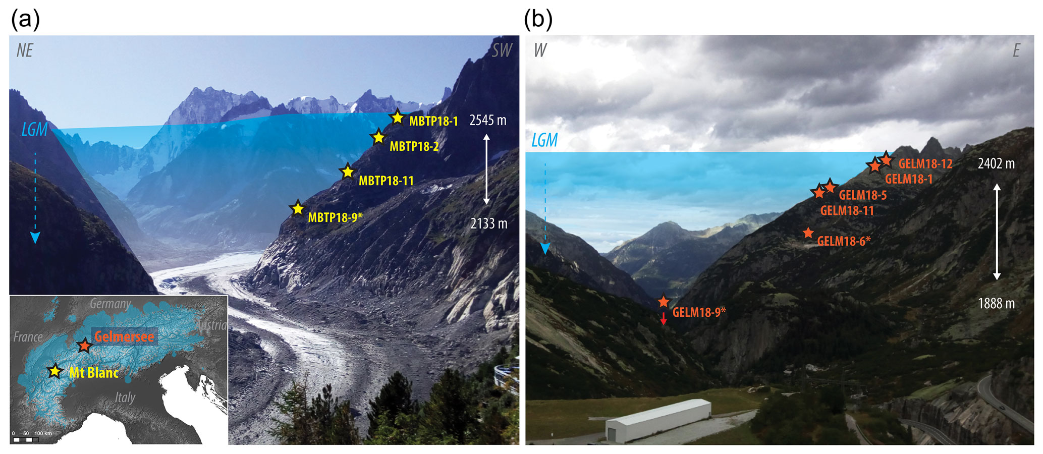
Figure 1Mont Blanc Trelaporte (MBTP, a) and Gelmersee (GELM, b) deglaciation profiles since the Last Glacial Maximum (LGM), with the spatial distribution of samples collected for quartz 10Be (Lehmann et al., 2020; Wirsig et al., 2016b) and 3He (this study) analyses. Samples with an asterisk have been exposed for ∼ 10–11 kyr (i.e., the entire Holocene period). The inset map indicates the location of the two study sites within the European Alps and the extent of ice cover during the LGM (in blue; Ehlers et al., 2011).
Ice-surface lowering of around 400 (MBTP) to > 500 (GELM) meters between the LGM and the YD has been recorded using in situ 10Be cosmogenic exposure dating on bedrock surfaces collected at regular intervals along each profile, starting from just below the trimline (Figs. 1 and 2, Table 1; Lehmann et al., 2020; Wirsig et al., 2016b). In this study, new samples were collected for 3He experiments from the same rock surfaces and locations as the sampling sites previously collected for 10Be dating by Lehmann et al. (2020; MBTP profile, samples MBTP18-1, -2, -11, and -9, n=4) and Wirsig et al. (2016b; GELM profile, samples GELM18-12, -1, -5, -11, -6, and -9, n=6; Fig. 1, Table 1). All samples are from glacially scoured bedrock surfaces, except GELM18-11, which comes from the top of a ∼ 5 m high boulder of similar lithology deposited during the post-LGM ice-surface lowering (Wirsig et al., 2016b).
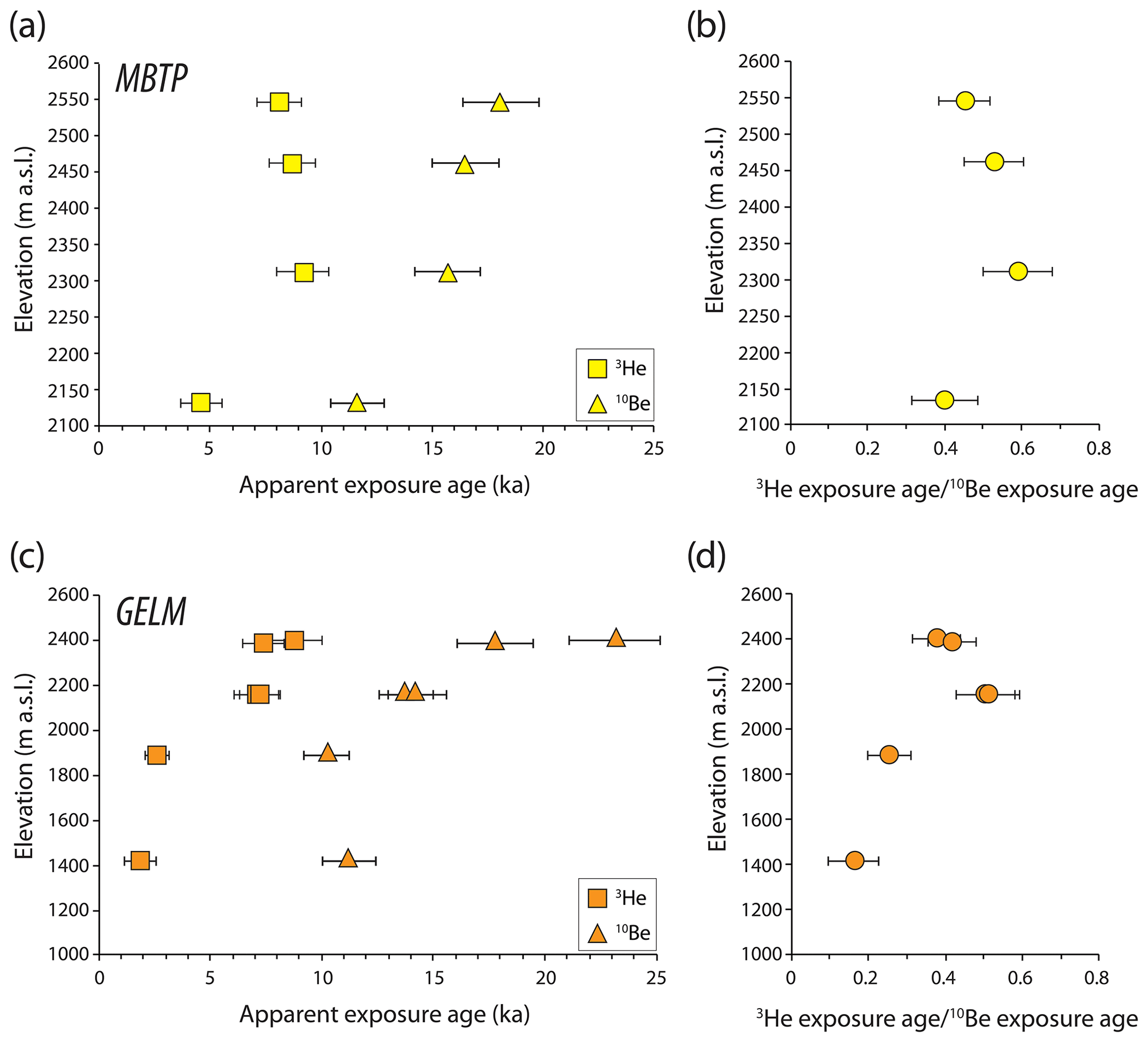
Figure 2Apparent quartz 3He (this study) and 10Be (Lehmann et al., 2020; Wirsig et al., 2016b) exposure ages (a, c), and exposure age ratios or retention (b, d) as a function of elevation along the two deglaciation profiles (MBTP: a, b; GELM: c, d).
Table 1MBTP and GELM sample information.
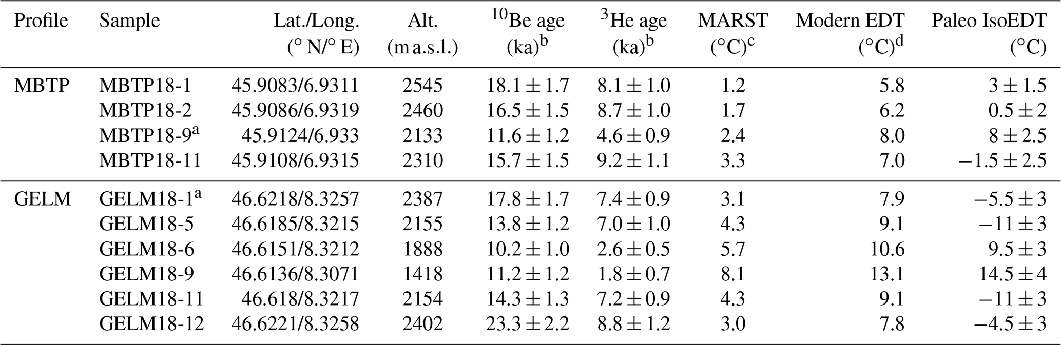
a Samples used for 3He diffusion experiments. b Re-calculated 10Be exposure ages (after Wirsig et al., 2016b and Lehmann et al., 2020) and calculated 3He apparent exposure ages using the non-time dependent scaling scheme of Stone (2000) and Balco et al. (2008), using SLHL production rates of 4.01 (10Be; Borchers et al., 2016) and of 116 (3He; Vermeesch et al., 2009) and assuming a rock density of 2.65 g cm−3. See the Supplement for the details of 10Be and 3He concentrations (Table S1 in the Supplement). c Estimated modern mean annual rock surface temperature (MARST) at ∼ 3 cm depth. d Modern effective diffusion temperature (EDT) calculated using Ea of 93.5 (MBTP) or 98.5 (GELM) kJ mol−1 and using 10 ∘C annual and 5 ∘C diurnal amplitudes. See Sect. 3.5 for the detailed explanation regarding modern MARST and EDT estimates.
In addition to measurements of cosmogenic 10Be, to determine the exposure time of a rock surface, cosmogenic 3He paleothermometry requires at least two additional types of measurement. First, we need measurements of the cosmogenic 3He concentration in the quartz, which permits us to estimate the amount of cosmogenic 3He loss by diffusion during the exposure of the rock surface. Second, we need to measure sample-specific 3He diffusivities for varying temperatures in our quartz samples by conducting stepwise-heating experiments.
We also need several different types of models to obtain paleotemperature estimates from these datasets. First, we need models to obtain diffusion kinetics parameters (i.e., activation energy, Ea, and the length-scale-normalized diffusivity at infinite temperature, also known as the pre-exponential factor, ; Tremblay et al., 2014a, b) from our stepwise-heating experiments. Some quartz samples, including the samples we study here, show complex 3He diffusion behavior that prevents us from using a simple linear model to extract diffusion kinetics parameters. In these cases, we model the diffusion kinetics parameters using the multiple diffusion domain (MDD) model framework (Lovera et al., 1989, 1991). Second, we forward model the production and diffusion of cosmogenic 3He over the duration of each sample's surface exposure for different thermal histories to compare the predicted 3He concentrations with the cosmogenic 3He concentrations observed in our samples. In order to account for diurnal and seasonal temperature oscillations, effective diffusion temperatures (EDTs, Tremblay et al., 2014a) are used as temperature inputs in the forward models.
We describe the measurement and modeling methods we used to apply cosmogenic noble gas paleothermometry to our samples as well as how EDTs were derived in greater detail below.
3.1 Sample preparation
Rock samples were disaggregated using a high-voltage, pulse-based system (SELFRAG equipment, Institute of Geological Sciences, University of Bern) to optimize the breaking of the rock along crystal grain boundaries. After rinsing, quartz mineral grains were separated from other minerals (heavy minerals and feldspar) by magnetic separation and froth flotation (e.g., Nichols and Goehring, 2019). The quartz separates were etched in 1 % HF for 3 weeks at room temperature to ensure the removal of any adhering micro-mineral particles that have the potential to contaminate the 3He measurements. For both sites, the grain size distribution is centered around a diameter of 850 µm after removal of the fraction finer than 200 µm (Fig. S1 in the Supplement).
For cosmogenic 3He measurements, the 800–1000 µm grain size fraction (i.e., 400–500 µm radii) from each quartz separate was selected. We chose this large grain size fraction, because we anticipated it would have best preservation potential of a measurable 3He signal, given the expected range of thermal histories experienced by the MBTP and GELM samples (Brook and Kurz, 1993; Tremblay et al., 2014a). Three replicates per sample consisting of ∼ 100 mg of quartz were prepared for analysis of natural 3He concentrations.
One representative sample per profile was selected for stepwise-heating experiments to determine diffusion kinetics parameters: MBTP18-9 and GELM18-1. For these samples, 200 to 300 mg of quartz grains were visually selected under a binocular microscope to avoid obvious mineral inclusions and fractures. The selected grains were sent to the Francis H. Burr Proton Therapy Center at the Massachusetts General Hospital for proton beam irradiation (Shuster et al., 2004; Shuster and Farley, 2005) in February 2019. After several months of rest to lower the level of radioactivity, one individual coarse quartz grain with no obvious fractures, mineral inclusions, or fluid inclusions was selected from each irradiated sample to conduct stepwise-heating experiments. The grain selected from MBTP18-9 had a ∼ 700 µm diameter, while the grain selected from GELM18-1 had a ∼ 900 µm. Grain diameters were estimated using calibrated petrographic microscope measurements.
3.2 Helium measurements
Both bulk degassing measurements to determine the natural cosmogenic 3He abundances and the stepwise-heating experiments on proton-irradiated quartz grains to characterize 3He diffusion kinetics were carried out at the BGC Noble Gas Thermochronometry Lab (Berkeley, USA). The measurements were conducted with an MAP 215-50 sector field mass spectrometer following a similar procedure to Tremblay et al. (2014b). For bulk degassing measurements, the samples were packaged into tantalum packets and heated in two, 15 min-long heating steps at 800 and 1100 ∘C with a diode laser, with temperature of the tantalum packet measured by pyrometry. The amounts of 3He and 4He released from each heating step were measured (Tables S1–S3). Hot blanks on empty tantalum packets were also analyzed, from which an averaged 3He blank correction of 7.7 × 10³ atoms was obtained. No 3He above blank levels was observed in any of the 1100 ∘C heating steps. For stepwise-heating experiments on proton-irradiated grains, the selected grains were placed in contact with the tip of a bare wire K-type thermocouple inside small platinum–iridium (PtIr) packets. The PtIr packets were heated with a diode laser in a feedback control loop with the thermocouple. Each experiment included over 30 to 40 heating steps of varying durations, with heating step temperatures between 70 and 550 ∘C and including at least one retrograde heating cycle (Tables S4 and S5). Blank measurements at room temperature were regularly conducted throughout the experiments for background subtraction from the measured raw signals, with averaged 3He blank corrections of 2.1 × 10⁴ atoms (MBTP18-9) and 4.9 × 10⁴ atoms (GELM18-1).
3.3 Diffusion kinetics determination
To obtain diffusion kinetics parameters (Ea and ) from the stepwise-heating experiments on proton-irradiated grains, we followed a multi-step procedure. For each proton-irradiated sample (one per site), we first produced an Arrhenius plot displaying the natural log of diffusivity D (scaled to the diffusion length scale a) as a function of inverse temperature (Fig. 3), calculated from the observed 3He release fractions using the equation of Fechtig and Kalbitzer (1966; in Tremblay al., 2014b). The Arrhenius plots for both samples are shown in Fig. 3. In the case of simple diffusion behavior that follows an Arrhenius relationship, all data points would form a single linear array in this plotting space, and single values of Ea and ) could be obtained from the slope and intercept of a linear fit, respectively. However, the Arrhenius plots for both samples show deviations from linearity (Fig. 3).
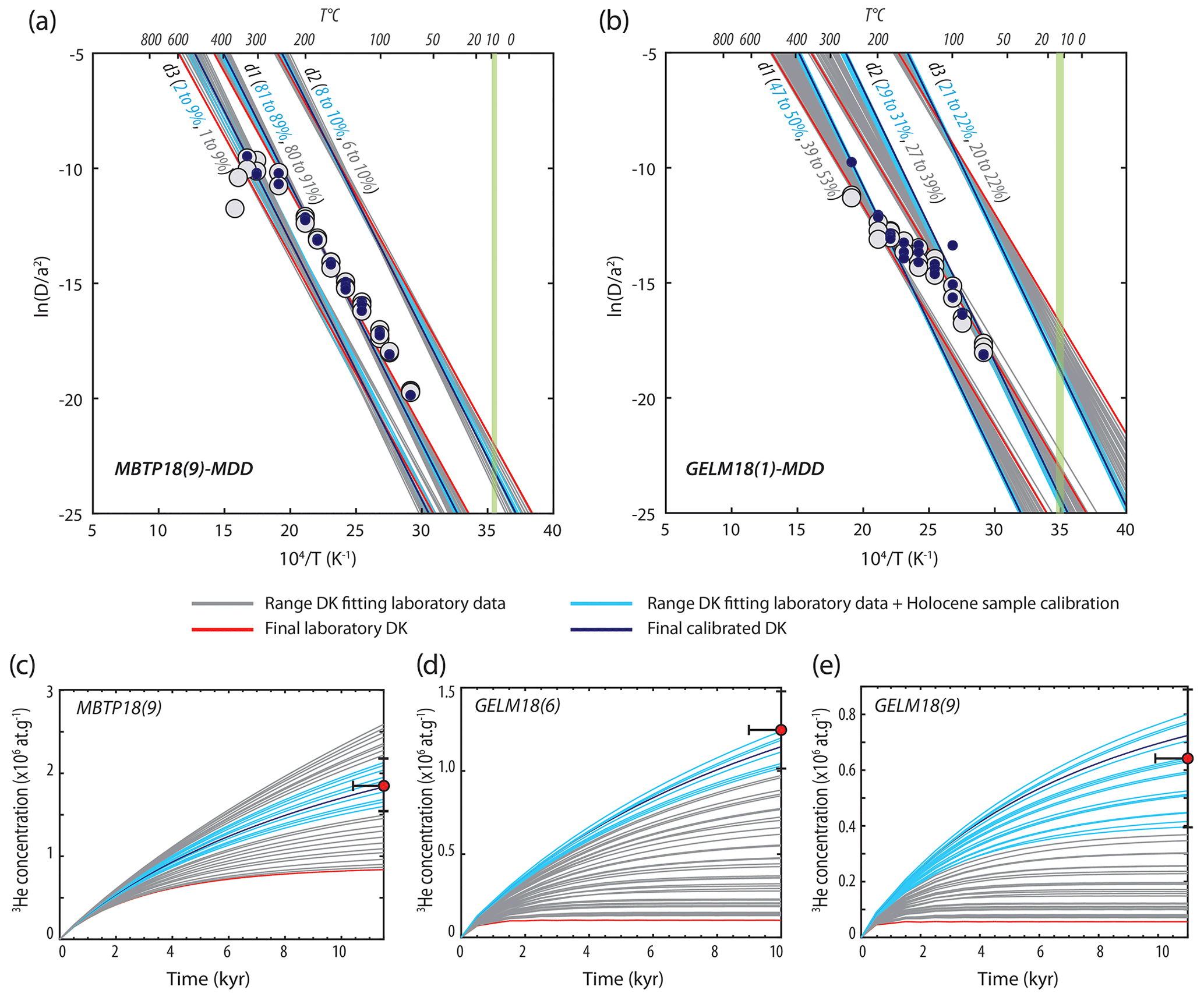
Figure 3Arrhenius plots of 3He step-degassing experiments conducted on one representative sample per study site (a: MBTP18-9, b: GELM18-1). Gray circles show values calculated from the laboratory experiments after Fechtig and Kalbitzer (1966). Diffusion kinetics (DK) parameters were calculated using a multi-step procedure. First, we fit the laboratory data assuming a range of Ea values (79 a and 86 b to 100 kJ mol−1; gray lines) for a three-domain MDD model. The red lines show three-domain DK parameters that minimize the misfit between the observed and predicted diffusivities (Ea is proportional to the slope of each line, and is given by the intercept). Second, we assessed whether these three-domain DK parameters could predict the cosmogenic 3He concentrations recorded in the Holocene calibration samples (c: MBTP18-9, d: GELM18-6, and e: GELM18-9). The three-domain DK parameters that could reproduce the Holocene calibration data are represented with light blue lines, with the dark blue line indicating the final calibrated DK parameters producing the best match with the natural Holocene 3He concentration(s). The small black circles in panels (a) and (b) represent the values modeled along the heating experiment schedule for this best-fit set of three-domain DK parameters. The vertical green line in panels (a) and (b) indicates the modern effective diffusion temperature (EDT) associated with the Holocene calibration sample(s). The gas fraction assigned to each domain for both laboratory-only (gray) and Holocene-calibrated (blue) DK parameters is also indicated along the model lines in panels (a) and (b).
Given the observation of nonlinear Arrhenius behavior, we follow the approach of Tremblay et al. (2014b) and use a multi-diffusion domain (MDD; Lovera et al., 1989, 1991) model framework to determine quartz 3He diffusion kinetics parameters for each study site. In the MDD framework, 3He diffusion is modeled as occurring in several non-interacting domains, with different effective diffusion length scales within the quartz grain (e.g., sub-grain fragments). Such a model can reproduce an observed nonlinear Arrhenius behavior and has been shown to be consistent with cosmogenic 3He observations in a geologic case study (Tremblay et al., 2014b). We use the code from Tremblay et al. (2021) to perform the MDD analysis on our stepwise-heating experiment data.
Preliminary MDD calculations were carried out to determine the Ea that best fitted the Arrhenius data points in the lower temperature range (∼ 70 to 100 ∘C), assuming a single diffusion domain, as well as the (minimum) number of diffusion domains to explain the entire dataset (i.e., all heating steps). Additional iterative runs using the MDD model with the minimum number of domains inferred from the preliminary tests were then conducted for a range of increasing Ea up to 100 kJ mol−1 (with a 0.5 kJ mol−1 increment; Fig. 3). This range of Ea values is based on existing Ea estimates reported for quartz in the literature (Shuster and Farley, 2005; Tremblay et al., 2014b, 2018; Domingos et al., 2020). In each run, Ea was kept common to each domain (Lovera et al., 1991; Baxter, 2010), while and the gas fraction for each different domain were allowed to vary until the misfit coefficient was minimized between the simulated and observed values for all the heating steps.
Stepwise-heating experiments conducted in a laboratory do not permit us to observe 3He diffusion behavior at Earth surface temperature range (i.e., from around −30 to 30 ∘C). Considering this fact, we introduced an extra calibration step that uses the measured natural 3He concentration from the samples with Holocene-only exposure (from both GELM and MBTP sites) to constrain the diffusion kinetics previously inferred from MDD models. The rationale for this is as follows: based on independent global and regional paleoclimate proxy records, samples exposed during the Holocene have experienced relatively stable average temperature conditions, with only minor variations (i.e., less than 2 ∘C; see Sect. 1). Assuming no complex exposure history, the 3He signal recorded in these samples should therefore be representative of 3He diffusion occurring at a constant temperature equivalent to the modern effective diffusion temperature (EDT) at each sample site (see Sect. 3.4 for full definition of EDT). We thus tested whether the sets of diffusion kinetic parameters from the MDD models could explain the natural 3He concentrations recorded in the Holocene samples from our two study sites (MBTP18-9, 10Be exposure age of ca. 11.6 ka; GELM18-9 and -6, 10Be exposure ages of ca. 10.2 and 11.2 ka). For each set of MDD diffusion kinetics parameters that minimized the misfit with the stepwise-heating experiment data, we used a forward model of 3He production and diffusion (Tremblay et al., 2021) to predict the concentration of 3He that would be expected for an exposure duration equivalent to the recalculated 10Be exposure age and for a constant temperature equivalent to the modern EDT of the Holocene sample(s) (insets Fig. 3). Diffusion kinetics parameters for which the modeled 3He concentration matched the observed cosmogenic 3He concentration in the Holocene calibration sample within error were retained. We considered the diffusion kinetics parameters that yielded the best match as the final calibrated diffusion kinetics parameters (Fig. 3). We assume that the Holocene-calibrated diffusion kinetics parameters apply to all the samples collected along each profile and use these diffusion kinetics parameters in subsequent calculations. We justify the assumption of common diffusion kinetics for samples from a same valley profile by the homogenous lithology observed between those samples.
3.4 Forward models of 3He production and diffusion
To explore what thermal histories could explain the observed cosmogenic 3He abundances in our quartz samples, we forward model the production and diffusion of cosmogenic 3He over the duration of each sample's surface exposure for different time–EDT scenarios using the approach of Tremblay et al. (2021). We model 3He production by cosmic ray incidence using a 3He production rate in quartz at sea level and a high latitude (SLHL) of 116 (Vermeesch et al., 2009), scaled to the sample geographic location and elevation according to the non-time-dependent scaling scheme of Stone (2000) and Balco et al. (2008). The duration of 3He production and diffusion in the simulations is constrained by each sample's 10Be exposure age. For consistency, the SLHL production rate of 10Be (4.01 by neutron spallation; Borchers et al., 2016) is also scaled with the Stone (2000) scaling scheme. Apparent 3He and 10Be exposure ages along the deglaciation profiles investigated in this study are (re-) calculated using the measured 3He (this study) as well as 10Be concentrations reported in the literature (previous studies, Wirsig et al., 2016b; Lehmann et al., 2020), assuming negligible erosion (Fig. 2; Tables 1 and S1).
3.5 Effective diffusion temperature estimates
Rock surfaces experience temperature fluctuations at the diurnal, seasonal, and longer (1 to 105 years) timescales, which will all activate thermal diffusion of 3He in quartz (Tremblay et al., 2014a). Because 3He diffusivity increases exponentially with temperature, a constant model temperature required to explain a total 3He loss (i.e., corresponding to the mean diffusivity through time) from a geological sample will equal or exceed the actual mean temperature experienced at the rock surface. This temperature is called effective diffusion temperature (EDT; Christodoulides et al., 1971; Tremblay et al., 2014a) and is a function of the 3He diffusion activation energy Ea, the long-term mean (rock surface) temperature, and the different frequency temperature amplitudes.
We estimated the modern EDT at the different sampling sites as follows. Mean annual air temperatures (MAATs) at each sampling site along the MBTP and the GELM profiles were calculated by linear interpolation, assuming a lapse rate of 5 (Grämiger et al., 2018) based on mean annual temperatures recorded by nearby reference weather stations at Chamonix (1042 , ∼ 5 km west; period 1993–2012; Magnin et al., 2015a) and Grimsel-Hospiz (1980 ; ∼ 5 km south; period 2010–2020, data MeteoSwiss), respectively. Mean annual rock surface temperatures (MARSTs) are typically higher than MAATs, with the difference amplified between south- and north-exposed slopes (Gruber et al., 2003). Boeckli et al. (2012a), based on 57 sensor measurements on snow-free rock slopes > 55∘, showed that the measured difference between MAAT and MARST increased linearly from < 1 to up to 10 ∘C, depending on potential incoming solar radiation (PISR), which is largely controlled by rock surface aspect and angle in addition to elevation. For moderately inclined surfaces, the difference between MARST and MAAT is expected to be reduced by ∼ 1–3 ∘C due to micro-topography and snow-insolating effects (Hasler et al., 2011). To estimate MARSTs, we calculated the PISR at each sampling site using the area solar radiation tool (ArcGIS software, version 10.3.1) applied to a 30 m resolution digital elevation model (SRTM 1 Arc-Second data) at the study sites. The calculation was performed at hourly resolution using data from 1 year (2000), assuming no nebulosity and using a sky size of 512 cells (Magnin et al., 2015a; Mair et al., 2020). Based on the linear relationship between MAAT–MARST and PISR from Boeckli et al. (2012a), we estimated the average MARST–MAAT difference, assuming snow-free conditions at each site, from which we then subtracted 2 ∘C to take into account snow-insulating and micro-topographic effects in moderately steep terrain (Hasler et al., 2011). Final differences between MAAT and MARST of +1 and +2.5 ∘C were thus obtained for the north-exposed MBTP and the southwest-exposed GELM sites, respectively. These estimates are consistent with in situ MAAT and MARST measurements available in nearby areas with similar orientations, elevations, and slope inclinations (e.g., Gruber et al., 2004; Magnin et al., 2015a, b; Haberkorn et al., 2017; Grämiger et al., 2018; Guralnik et al., 2018) and were thus used to estimate the MARSTs at each sampling site.
Table 2Diffusion kinetics parameters for MBTP and GELM sites.
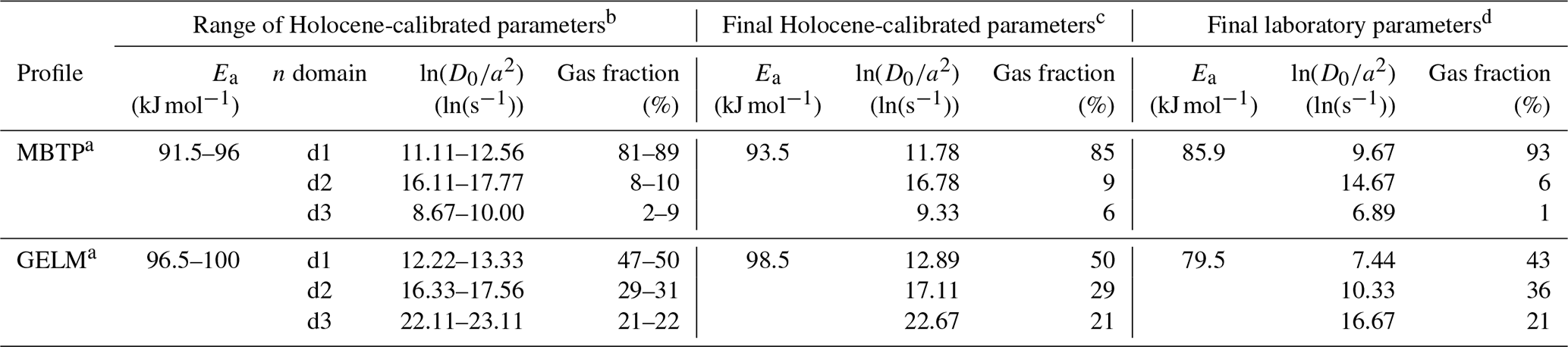
a Diffusion kinetics measurements made on one representative sample per profile: MBTP18-9 (350 µm spherical equivalent radius) and GELM18-1 (450 µm spherical equivalent radius). b Range of MDD diffusion kinetics parameters obtained by fitting laboratory experimental data and matching 3He concentrations (within 1σ error) from Holocene calibration samples. c Best-fitting MDD diffusion kinetics parameters obtained by fitting laboratory experimental data matching 3He concentrations from Holocene calibration samples. d MDD diffusion kinetics parameters based only on laboratory experimental data and providing the best match in the lower temperature range of the heating schedule (∼ 70–100 ∘C).
A mean annual temperature amplitude of 10 ∘C and diurnal amplitude of 5 ∘C were adopted for the two sites, based on long-term (i.e., several years) temperature records from the Chamonix and Grimsel-Hospiz weather stations and from direct in situ rock surface measurements available in the Alps (Gruber et al., 2004; Magnin et al., 2015b; Grämiger et al., 2018; Guralnik et al., 2018; Mair et al., 2020). These estimates are consistent with the annual and diurnal amplitudes obtained from the spatially interpolated land surface climate dataset, WorldClim 2.0, based on gridded time series of meteorological data from available weather stations (target temporal range 1970–2000; 1 km resolution; Fick and Hijmans, 2017).
Past colder EDT inputs in forward 3He modeling for varying thermal histories are based on temperature anomalies from modern EDTs.
First, we examine the characteristics of the 3He diffusion kinetics parameters we modeled for our quartz samples and explore the sensitivity of the 3He signal in those samples to Earth surface EDTs. We then present forward model results for the evolution of the cosmogenic 3He concentrations recorded along each deglaciation profile for two different sets of thermal histories. The first set of thermal histories we investigate assumes a constant EDT since the exposure of the sampled rock surfaces following ice retreat. We then investigate a set of more climatologically interesting thermal histories, wherein a change in EDT occurs at some point during the exposure time of each sample.
4.1 Diffusion kinetics and sensitivity tests
Figure 3 shows the range of diffusion kinetics parameters (Ea and ln( that fit the laboratory stepwise-heating experiments (one representative sample for each site; Fig. 3a and b) and which permit us to reproduce the observed natural 3He concentrations from the Holocene calibration samples for a constant EDT equivalent to the modern EDT (Fig. 3c–e). Stepwise-heating experiment data indicate relatively first-order Arrhenius behavior for quartz 3He diffusion of MBTP18-9, with one dominant linear array accounting for ∼ 85 % of 3He release (Fig. 3a, Table 2). The remaining ∼ 15 % gas fraction is distributed within two additional minor diffusion domains, one of higher retentivity and one of lower retentivity (Tremblay et al., 2014b). GELM18-1 exhibits more complex quartz 3He diffusion behavior, with gas release distributed more equally between three linear arrays (Fig. 3b, Table 2) that can be interpreted as three or more distinct diffusion domains, with each domain contributing significantly to 3He retention over geological times.
In order to explore the theoretical sensitivity (and potential variability) of the MBTP and GELM quartz, we numerically evaluated the time required for the concentration of 3He in each sample to reach steady-state conditions (i.e., thermal loss balanced with cosmic-ray induced production gain) as a function of constant EDT. Forward simulations of 3He production and diffusion (Tremblay et al., 2014a, b, 2021) using the final Holocene-calibrated diffusion kinetic parameters were thus run for a range of isotherms representative of Earth surface EDTs (hereafter referred to as isoEDTs; tested range from −30 to 30 ∘C), assuming a 450 µm radius and no initial 3He concentration. Equilibrium conditions were assumed to be reached once no significant change in 3He concentration was recorded (< 1 % kyr−1). While we observe some variability in 3He diffusion behavior and derived diffusion kinetics parameters between MBTP and GELM quartz (Fig. 3, Table 2), results from sensitivity tests in terms of steady-state times are relatively similar. For isoEDTs between −10 and 10 ∘C, bracketing approximately potential EDT values experienced along both deglaciation profiles between the LGM and today, the time predicted for 3He diffusion to reach equilibrium varies between ∼ 10 kyr (isoEDT of 10 ∘C) and ∼ 20 kyr (isoEDT of −10 ∘C; Fig. 4). Interestingly, while steady-state time estimates remain relatively constant for quartz from both sites at ca. 20 kyr for colder isoEDTs (−10 to −30 ∘C), we observe a pronounced non-linear dependence for EDTs above 0 ∘C, resulting in much shorter equilibrium times in the high EDTs range (less than 5 kyr for EDT above 20 ∘C, Fig. 4).

Figure 4Theoretical 3He steady-state time estimates for isoEDTs varying between −30 and 30 ∘C using the final Holocene-calibrated diffusion kinetics parameters determined for each study site and assuming 450 µm grain radius.
4.2 3He exposure ages and PaleoIsoEDTs
For each site, apparent 3He exposure ages are systematically lower (from 20 % to 75 %) than apparent 10Be exposure ages (Table 1, Fig. 2). The 10Be ages show a general decrease with decreasing elevation, in agreement with progressive ice thinning along a deglaciation profile in the high Alps during the Late Glacial. This trend is less evident for the apparent 3He ages, which overlap significantly within uncertainties above ∼ 2200 (Fig. 2). The 3He retention ( exposure age ratio) shows a clear decrease with decreasing elevation along the GELM profile (∼ 1500 to 2500 ), which is not visible along the MBTP profile (similar retention between MBTP samples), which is also more restricted in elevation range (∼ 2100 to 2600 ; Fig. 2).
To determine the apparent constant EDT (that we refer to as paleoIsoEDT) from the natural 3He signal recorded in each sample, forward models of 3He production and diffusion (implemented with the final Holocene-calibrated diffusion kinetics) were run for a time period equal to the sample's 10Be exposure age and for a range of isoEDTs (isothermal holding between −10 and 15 ∘C for MBTP; −25 to 20 ∘C for GELM, 1 ∘C increment). The isoEDT leading to best-matching synthetic 3He concentration with the observed natural 3He concentration was retained as the paleoIsoEDT (Fig. 5, Table 1). As Holocene samples were used to calibrate the diffusion kinetics (see Sect. 4.1), it is expected that 3He-derived paleoIsoEDTs from these samples are equivalent to their respective modern EDTs. On the other hand, all pre-Holocene samples at both sites have paleoIsoEDTs that are lower than their corresponding modern EDTs (Fig. 5a and d; Table 1). For the MBTP profile, the difference between modern EDTs and paleoIsoEDTs varies from around 3 to 9 ∘C. This difference is even greater for the GELM profile, where paleoIsoEDTs are around 12 to 20 ∘C lower than their associated modern EDTs. Pre-Holocene samples are located well above (200 to 500 m) Holocene samples and all above 2000 . While paleoIsoEDTs derived from the high-elevation, pre-Holocene samples agree within error for each site, they clearly depart from paleoIsoEDTs obtained from the low-elevation, Holocene sample(s) by ∼ 6∘ (MBTP site) and ∼ 18 ∘C (GELM site), based on the peak values from the obtained bimodal probability distributions (Fig. 5b and e). After correcting for temperature decreases with elevation (assuming a lapse rate of 5 ), the difference in the paleoIsoEDTs between pre-Holocene and Holocene samples is still significant for GELM (∼ 10 to 20 ∘C, Fig. 5f). For MBTP, although elevation-corrected paleoIsoEDTs from two high-elevation, pre-Holocene samples (MBTP18-2 and -11) are still clearly distinguishable from the low-elevation, Holocene sample (MBTP18-9; Fig. 5c), the probability distribution appears closer to unimodal, since the paleoIsoEDT from the highest sample (MBTP18-1) partially overlaps that from MBTP18-9 within uncertainty.
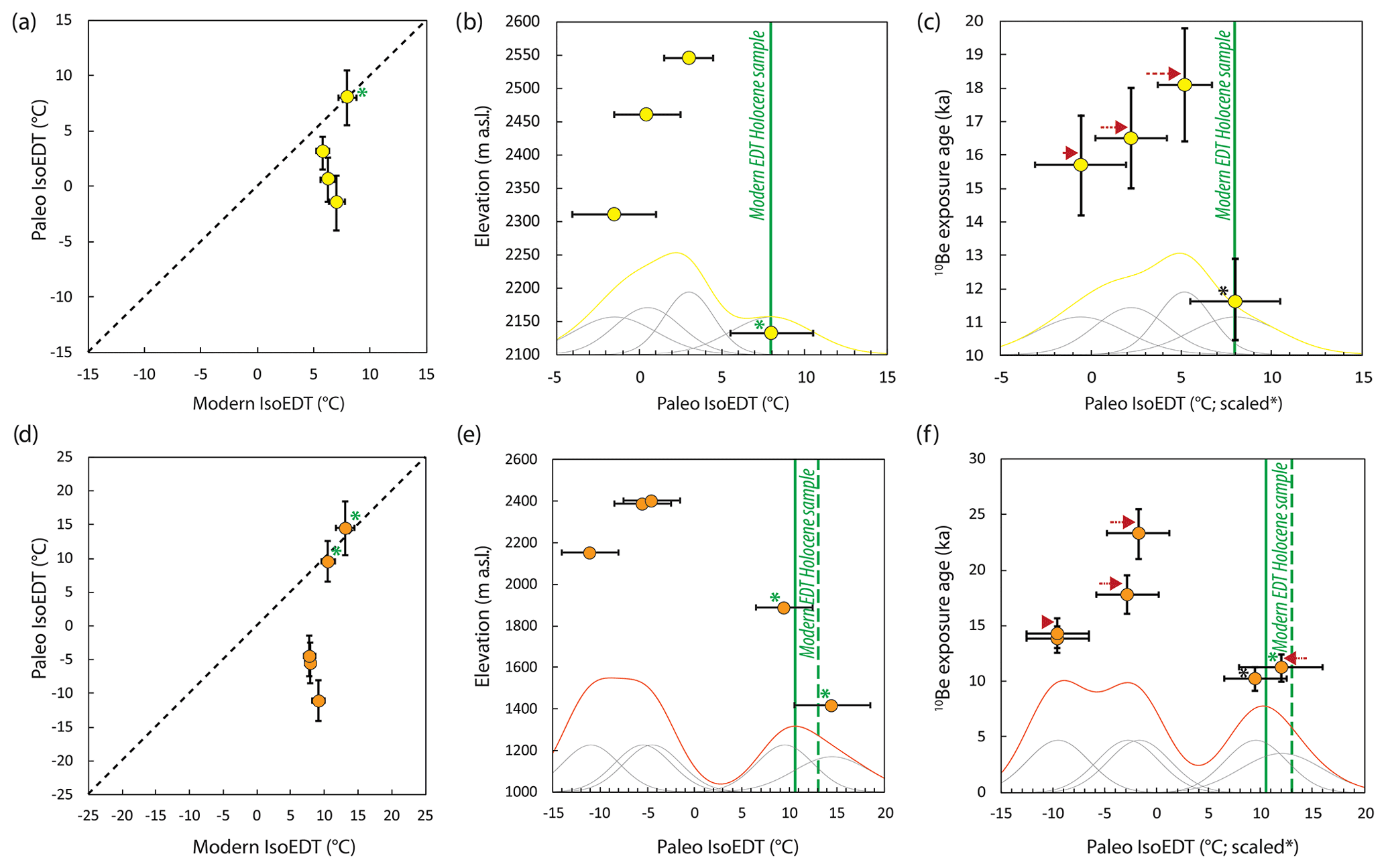
Figure 5Distribution of 3He-derived paleoIsoEDTs along the MBTP (a–c) and GELM (d–f) deglaciation profiles. Holocene samples used for calibration are marked by asterisks. (a, d) PaleoIsoEDTs relative to modern EDTs (black dashed line is 1:1); (b, e) relationship between paleoIsoEDT and elevation; and (c, f) relationship between paleoIsoEDT and 10Be exposure age after correction for lapse rate (marked by red arrows, relative to the Holocene sample marked with a black asterisk). Green solid and dashed lines are modern EDTs for Holocene samples, with the solid line indicating the modern EDT taken as reference for the lapse rate correction. The thin lines represent the sums (yellow and orange) of the individual (gray) probability distributions of paleoIsoEDTs.
4.3 Forward simulations with time-varying EDT
Based on global and regional paleoenvironmental records, we can expect that pre-Holocene samples collected at the MBTP and GELM sites have experienced at least one main significant temperature change, marking the transition from (colder) Late Glacial to warmer and more stable Holocene conditions (cf. Sect. 1 for details).
Following this observation, we first investigate the theoretical time needed for the MBTP and GELM 3He quartz systems to re-adjust to a change in temperature for a warming scenario, assuming that these systems were already at steady-state conditions. Forward model simulations (450 µm radii assumed) were run for different time–EDT scenarios involving an initial EDT (ranging from −30 to 30 ∘C; initial 3He concentration at steady state with initial EDT) followed by a step-warming event (+2, +5, +10 +15, +20, +25, +30 ∘C; over 0.1 to 1 kyr, depending on the sensitivity of the quartz system for the considered EDT scenario), after which the resulting warmer EDT was maintained until full re-adjustment of the 3He-quartz system. We considered full re-adjustment to have occurred when modeled 3He concentrations following the step-warming event matched within 10 % the 3He concentrations expected for an isoEDT equivalent to the final (warmer) EDT (Fig. 6a). We present simulation results in Fig. 6b and c. For past EDTs < 0 ∘C followed by a step warming up to 20 ∘C, readjustment times are all longer than 10 kyr, considering either MBTP or GELM diffusion kinetics. Estimates of LGM-temperature anomalies suggested for the European Alps are equivalent to an apparent warming of 5 to 15 ∘C (see Sect. 1). When considering EDT scenarios with a similar warming range applied to our study sites, with modern EDTs around 5 to 10 ∘C (at pre-Holocene sampling sites; i.e., equivalent to initial past EDT of 0 to 5 and −10 to −5 ∘C for 5 and 15 ∘C warming step, respectively), our simulation outcomes show relatively long re-adjustment times from around 20 to 45 kyr (Fig. 6). We should note, however, that these times are maximum estimates, since we considered 3He quartz systems at steady-state conditions with initial cold EDTs before the warming event.
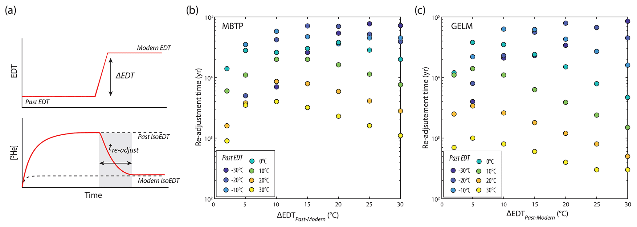
Figure 6Conceptual approach (a) and output results for MBTP (b) and GELM (c) of 3He re-adjustment time (tre-adjust) for one-step EDT change scenarios (temperature warming from 2 to 30 ∘C), using the final diffusion kinetics parameters determined for each study site and assuming 450 µm grain radius. Calculations assume that 3He concentrations were already at steady state for past EDT conditions (i.e., as would be expected for infinite exposure time) prior to imposing the temperature change.
In a second set of forward model runs, we explore the thermal memory of 3He in quartz for a step-warming EDT scenario fixed in time that is more representative of the post-LGM paleoclimate history in the Alps, including: (1) an initial cold period starting at 24 ka, with an imposed EDT set 15 ∘C lower compared to modern EDT (maximum LGM temperature anomalies, see Sect. 1); (2) a warming step to modern EDT that is either progressive from 24 to 10 ka or abrupt between 11 and 10 ka (i.e., consistent with a Younger Dryas–Holocene transition); and (3) stable conditions at the modern EDT throughout the Holocene (lasty10 kyr, Fig. 7a). Forward simulations of 3He diffusion and concentration evolution were conducted for each pre-Holocene sample following this scenario, with the time period and the time-dependent EDT variable set accordingly to each sample 10Be exposure age and modern EDT, respectively. For all GELM and MBTP samples, these forward simulations result in synthetic 3He concentrations significantly lower than their respective measured 3He concentrations. In Fig. 7b, we present the results for sample MBTP18-1, for which we observed the smallest difference between modern EDT and paleoIsoEDT (Fig. 5a; Table 1).
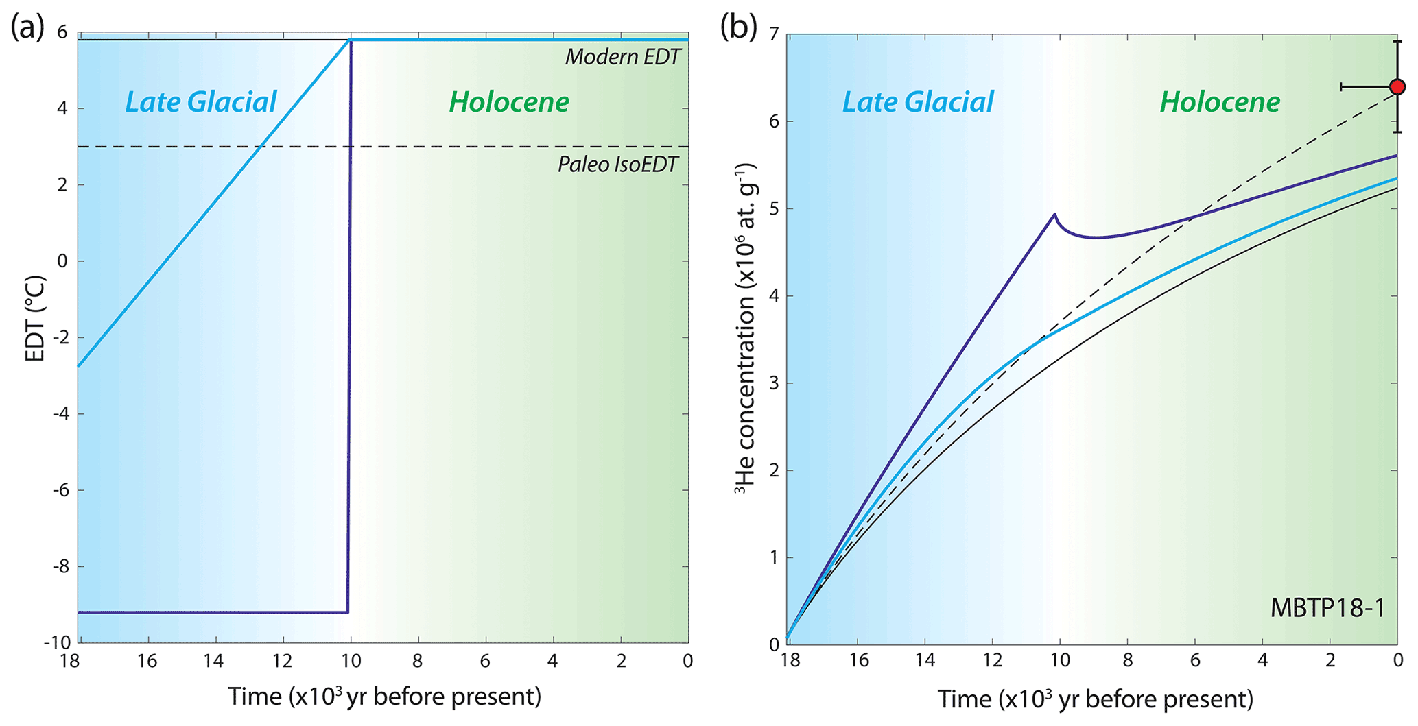
Figure 7(a) Simplified warming EDT scenario since the LGM (∼ 24 ka), with progressive and abrupt EDT changes in light and dark blue lines, respectively; (b) synthetic evolution of 3He concentration (blue lines) compared with the natural 3He concentration recorded in MBTP18-1 (red circle). The 3He concentration evolution is also indicated for a constant-temperature scenario at the modern EDT and paleoIsoEDT (set in Fig. 5; black solid and dashed lines, respectively). We were unable to reproduce the observed natural 3He concentration for any samples with pre-Holocene exposure under this simplified LGM EDT scenario.
To further investigate potential effects of a larger EDT differences between modern and past conditions and/or a more recent EDT change, we performed an additional set of numerical simulations using step-warming EDT scenarios with more free parameters. Scenarios with an EDT change occurring from 104 to 102 years ago and with a difference between past and modern EDTs (ΔEDT) up to 40 ∘C were tested iteratively on each pre-Holocene sample, assuming no initial 3He concentration and with total exposure time and EDT variables adjusted accordingly, as described above. Scenarios for which we could reproduce the observed natural 3He concentration (within uncertainties) were accepted, resulting in a range of different possible scenarios with varying ΔEDT and time of EDT change for each pre-Holocene sample (Fig. 8). For both sites, we observed a similar pattern between ΔEDT and time of EDT change: the further back in time the EDT change occurs, the greater the ΔEDT that is needed to reproduce observed natural 3He concentrations. In addition, for any given time of EDT change, ΔEDTs tend to be inversely correlated with sample elevation and 10Be exposure age. Within these similarities, the two sites differ by the magnitude of the ΔEDT required to reproduce observed natural 3He concentrations. For example, along the MBTP site (Fig. 8a), ΔEDTs of 5 ∘C occurring a few kyr ago are required to explain 3He concentrations measured in the highest and/or oldest sample (MBTP18-1), while ΔEDTs of 35 ∘C occurring a few kyr ago are required to explain 3He concentrations measured in the lowest and youngest pre-Holocene sample (MBTP18-11). For the same sites, ΔEDTs of 3 and 15 ∘C are required if the ΔEDT occurred within the last centuries. On the other hand, for the GELM site, our simulations found no ΔEDT solution if the EDT change is applied prior to 1 ka (within our ΔEDT limit of 40 ∘C; except for GELM18-12; Fig. 8b). In the case of EDT change occurring within the last centuries, ΔEDTs for the GELM samples are significantly larger than for MBTP samples, with ΔEDTs between 15 and > 30 ∘C required for the highest and/or oldest samples (GELM18-12 and -1). For the intermediate samples (GELM18-11 and -5), which also exhibit the greatest 3He-10Be age differences, numerical solutions could only be recovered for very recent EDT changes (≤ 200 yr) and with ΔEDT > 35 ∘C.
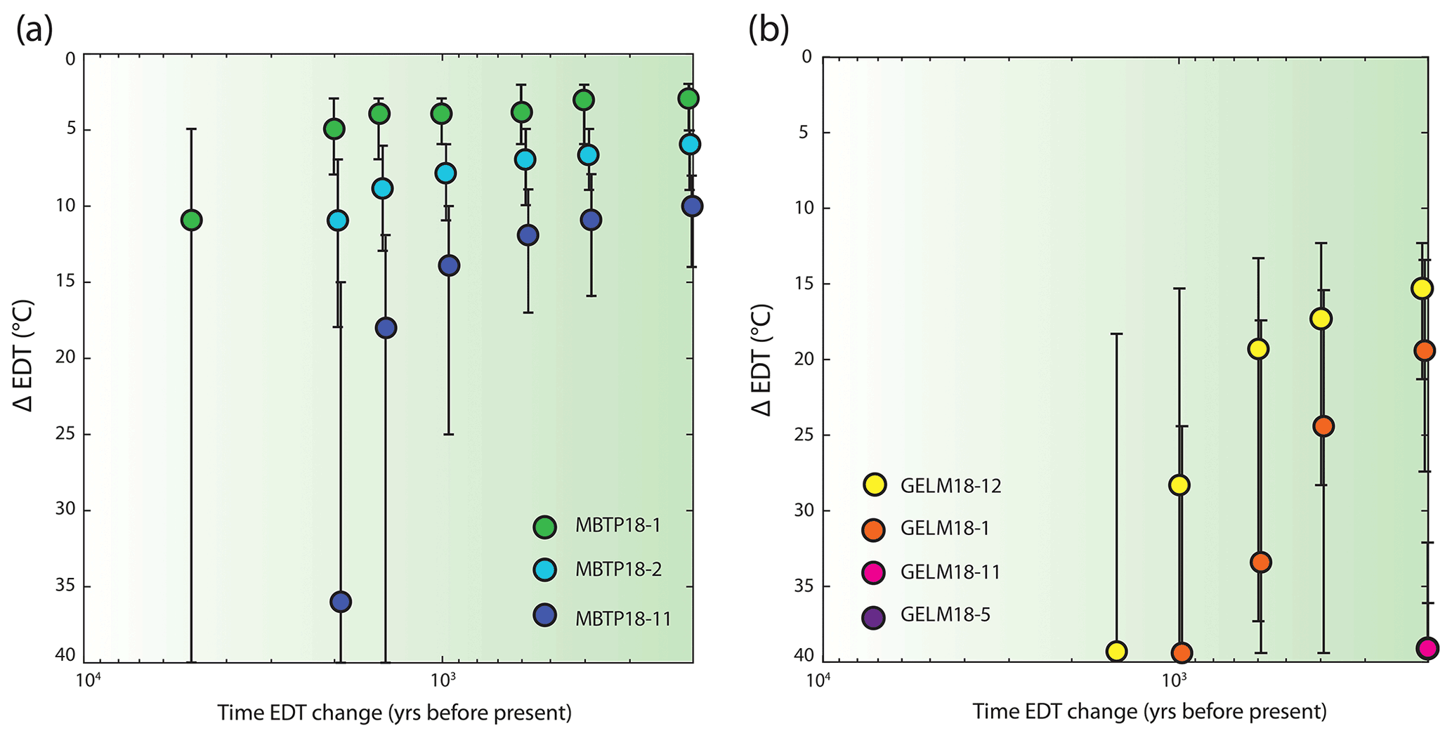
Figure 8One-step EDT change scenarios that reproduce the observed natural 3He concentration for each pre-Holocene MBTP (a) and GELM (b) sample, with ΔEDT solution as function of the time of EDT change. The error bars indicate all the possible ΔEDT solutions and the color circles indicate the best-matching scenario.
5.1 Paleoclimatic interpretation of 3He signals
All studied samples indicate the preservation of a 3He concentration consistent with temperatures that are colder than present-day EDT conditions at both the MBTP and the GELM sites (paleoIsoEDTs ∼ 3–9 and ∼ 12–20 ∘C lower than modern EDTs, respectively, Fig. 5). However, for both sites, the recorded 3He concentrations are apparently not concordant with simple time–EDT scenarios describing a plausible post-LGM mean temperature evolution in the European Alps (i.e., LGM mean temperature anomaly up to 15 ∘C, Fig. 7). Even when allowing for a larger EDT difference between LGM and the present day (up to 40 ∘C), modeled 3He concentrations remain significantly below the observed values at both sites. Such large EDT differences would not be supported by any set of mean temperature reconstructions for the European Alps since the LGM (e.g., Heiri et al., 2014a). Likewise, potential variation in seasonal temperature cannot contribute significantly to a larger pre-Holocene EDT anomaly. Indeed, global and regional paleoclimate studies rather suggest that a larger seasonal temperature amplitude occurred before the Holocene (e.g., Davis et al., 2003; Buizert et al., 2018), which would have the effect of increasing the paleoEDTs instead (Fig. 9).
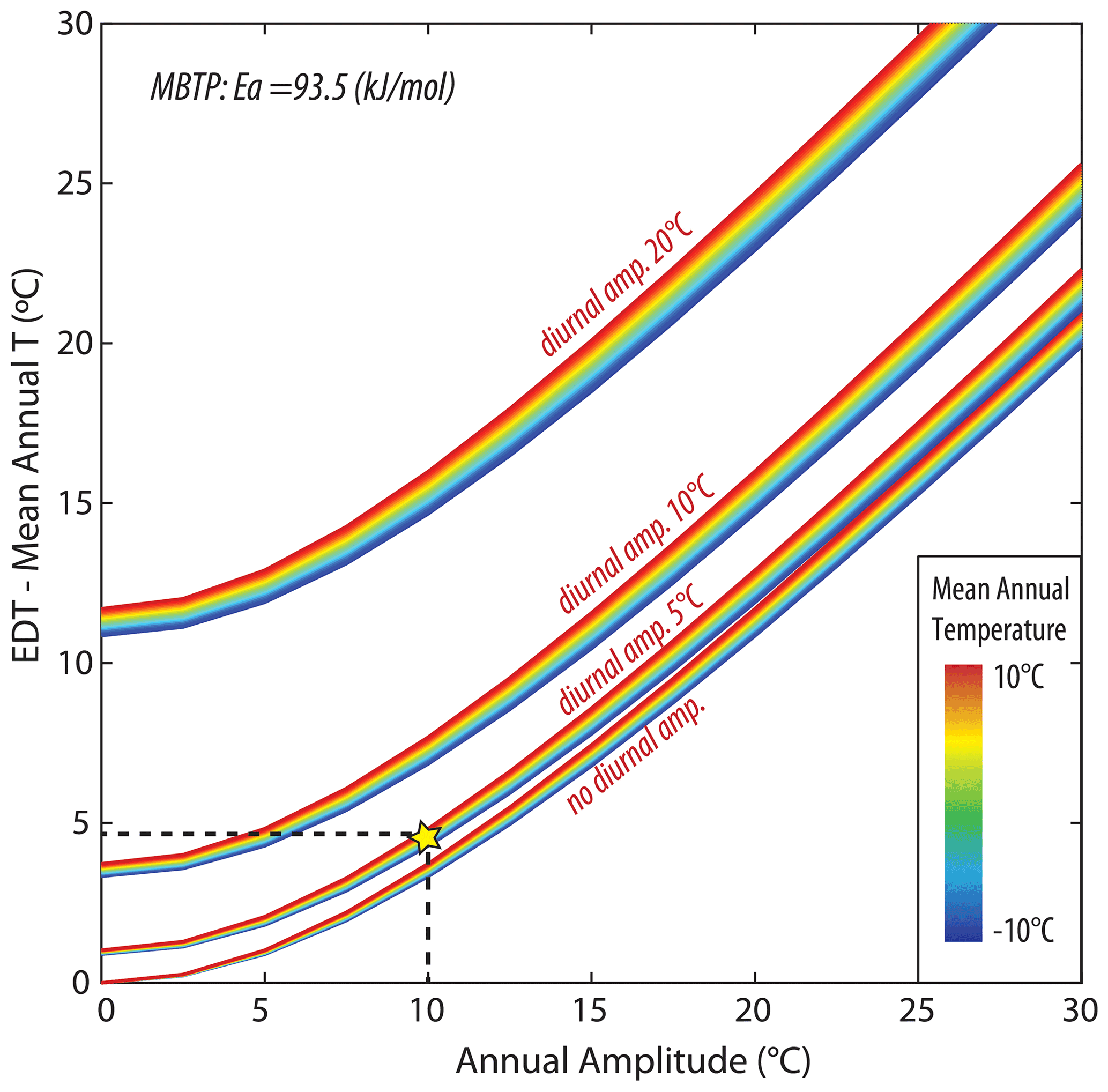
Figure 9Difference between EDT and mean annual temperature as a function of increasing seasonal temperature amplitude for different diurnal temperature amplitudes and assuming an Ea of 93.5 kJ mol−1 (MBTP site, Holocene-calibrated diffusion kinetics). The yellow star indicates the conditions used to estimate the modern EDT at the sampling sites. Decreasing the annual and/or diurnal amplitude can yield to up to a ∼ 5 ∘C decrease in the modern EDT. Similar results are obtained when using Ea = 98.5 kJ mol−1 (GELM site, Holocene-calibrated diffusion kinetics).
We attribute the result of modeled 3He concentrations that are significantly lower than the observed ones to the damping effect of modeled exposure during the Holocene period, which is characterized by relatively stable mean temperature conditions similar to the present day. By damping effect, we mean that modeling ∼ 10 kyr of exposure at temperatures similar to today results in a partial to total readjustment of the cosmogenic 3He thermal signal, with little to no inherited signal memory of the prior exposure to colder Late Glacial conditions. This hypothesis appears to contradict our theoretical tests, which indicate that the 3He thermal signal inherited from past EDTs 10 to 15 ∘C colder than today should a priori be (partly) preserved for 30–45 kyr under modern EDT conditions (Fig. 6). However, this time range relies on the assumption that bedrock surfaces were exposed for long enough to past colder conditions before the temperature change occurred in order to reach 3He steady-state concentrations. For both sample sites, the time required to reach steady state is around 20 kyr (Fig. 4). On the other hand, along the MBTP and GELM profiles, bedrock surfaces have not been exposed for more than 5–8 and 4–13 kyr before the Late Glacial–Holocene transition, respectively. This results in 3He accumulation up to 35 %–55 % (MBTP) and 30 %–85 % (GELM) of 3He steady-state concentrations when considering paleoIsoEDTs 10–15 ∘C lower than present-day EDTs. In such a case, 3He re-adjustment time estimates to modern EDTs are predicted to be reduced by ∼90 % to 80 % for the MBTP site and by >90 % to 60 % for the GELM site, implying we should recover the dominance of Holocene temperature conditions in the 3He signal from the sampled bedrock surfaces.
Our observed 3He concentrations can be reproduced by forward simulations with an EDT change occurring on much more recent timescales (Fig. 8). For the MBTP site, a ΔEDT of 7 to 5 ∘C within the last few thousand years to centuries predicts the observed natural 3He concentrations for two pre-Holocene samples: MBTP18-1 and -2. A ΔEDT of 12 to 8∘ is required for MBTP18-11. Such a ΔEDT estimate, considering mean temperature fluctuations up to 2 ∘C for the Holocene period (Davis et al., 2003), would also require variations in diurnal and/or annual temperature amplitudes to account for an additional 5 ∘C ΔEDT. However, this would imply the lowering of both diurnal and annual temperature amplitudes to null before modern conditions (Fig. 9), which contradicts global and regional records that indicate an increased seasonality in the early Holocene compared to the present day (Davis et al., 2003; Buizert et al., 2018) and which would result in a larger ΔEDT. Furthermore, the forward simulations discussed here used diffusion kinetics calibrated on Holocene samples (Fig. 8). Therefore, allowing a significant EDT change over the last 102–103 years is in contradiction with our calibration approach (see Sect. 3). If instead we use diffusion kinetics solely derived from laboratory experiments without Holocene calibration (Fig. 3, Table 2), a ΔEDT of 15 ∘C or greater is required to explain observed MBTP 3He concentrations for changes within the last 103 years (Fig. S2b). Such large ΔEDTs are significantly greater than expected EDT variations from changes in mean annual temperatures and/or in annual or diurnal temperature amplitudes during the Holocene. Even greater ΔEDTs are needed to explain the observed GELM 3He concentrations using either diffusion kinetics approach (Fig. S3b). Both cases are clearly incompatible with plausible Holocene paleoclimatic histories.
5.2 Sources of uncertainty
Cosmogenic 3He paleothermometry is still in an early stage of development for applications to Quaternary geology (Tremblay et al., 2014a, b, 2018), and there are several aspects of our approach that are under-constrained, which could contribute to our estimates of unrealistically cold Late Glacial temperatures. Below, we explore how uncertainties related to (1) estimating modern EDTs, (2) interpreting cosmogenic nuclide measurements, and (3) determining helium diffusion kinetics in quartz could each have affected our production–diffusion modeling and therefore our paleotemperature estimates.
5.2.1 Modern EDT estimates
Potential uncertainties in modern EDT estimates, used to define the EDT of the recent and stable period in the step-warming EDT scenarios (Sect. 4.3), cannot be ruled out. In particular, it is not known to what extent present-day conditions (based on decadal direct air and ground temperature measurements; see Sect. 3.1) are representative over centennial to millennial time scales. Correcting for overestimated diurnal and/or annual temperature amplitudes and/or mean annual temperatures would result in lower modern EDTs (Fig. 9). Assuming an overestimate of 50 % in modern diurnal and annual temperature amplitudes and up to 2 ∘C overestimate in MARST based on recorded mean temperature fluctuations (Davis et al., 2003; Ghadiri et al., 2018, 2020) and applied corrections to MAAT (see Sect. 3.1) would lead to ∼ 3.5 ∘C lowering of modern EDTs for MBTP and GELM sites. Applying such an estimated correction to the recent-period EDT potentially permits us to resolve observed 3He concentrations for two of the MBTP samples (MBTP18-1 and -2), with ΔEDT of 5 to 10 ∘C for a change occurring at ca. 10 ka (i.e., LGM scenario; Fig. S2c). It is also worth noting that natural 3He MBTP concentrations for those samples can be reproduced with minor ΔEDTs (≤ 1.5 ∘C) over recent timescales (102–103 years). When using laboratory-derived diffusion kinetics without Holocene calibration, a priori more appropriate to explore recent EDT changes, only scenarios with more than −10 ∘C ΔEDT within the last thousand years are accepted (Fig. S2d), inconsistent with paleoclimatic records over this recent time period. For GELM samples, correcting modern or recent EDT is not sufficient to reproduce the observed 3He concentrations with plausible ΔEDTs for an EDT change occurring at the Late Glacial–Holocene transition (ca. 10 ka; no solution) nor on more recent timescales (Fig. S3c and d).
5.2.2 Interpretation of cosmogenic nuclide measurements
Several sources of geological uncertainties may affect the results obtained in this study. First, our approach relies on the assumption that bedrock surfaces have experienced a simple exposure history along the time period recorded by 10Be concentrations, without pre-exposure or episodic coverage (i.e., non-erosive cold-based ice). Depth profiles of 10Be measurements on glacially polished bedrocks in the western Alps, with apparent exposure ages of 10–20 ka, indicate that an inherited 10Be concentration due to insufficient glacial erosion may persist and could lead to up to 9 % age overestimates (Prud'homme et al., 2020). Similarly, Wirsig et al. (2016b) suggested potential but limited pre-LGM (less than a few ka overestimate) inheritance for some GELM samples. While previous bedrock surface exposure would also imply an inherited 3He concentration, the latter would be subject to diffusion (partial or total) during glacier coverage, even at subzero temperatures and EDTs (Fig. S4). On the contrary, 10Be would experience only minor radioactive decay over 10–100 kyr timescales. This scenario of inheritance and/or complex exposure history would result in lower 3He concentrations recorded by bedrock surfaces regardless of the temperature history experienced by the rock surface during the total 10Be exposure period (i.e., lower concentration ratio; Balco et al., 2016). This scenario is also valid for post-LGM episodic coverage. Such effects are, however, expected to be minor, considering the limited potential 10Be inheritance (< 10 %) from pre-LGM exposure as well as the unlikelihood of prolonged coverage of the relatively steep (i.e., no loose sediments or thick snow accumulation) and high (i.e., above tree-line) sampled bedrock surfaces. Moreover, attempting to correct for these processes would result in opposite effects than what we observed for MBTP and GELM samples, with even lower paleoIsoEDT estimates and greater ΔEDTs required for warming EDT scenarios to recover observed natural 3He concentrations.
An additional source of uncertainty is postglacial erosion of sampled bedrock surfaces, assumed to be negligible in this study. Based on a combined approach exploiting cosmogenic 10Be and optically stimulated luminescence (OSL) systems, Lehmann et al. (2020) suggested potential high postglacial erosion rates (above 3.5 mm kyr−1) for low-elevation MBTP samples. Other regional estimates for crystalline bedrock commonly indicate Alpine postglacial erosion rates of 0.1 to 1 mm kyr−1 (Kelly et al., 2006; Dielforder and Hetzel, 2014; Wirsig et al., 2016b), which is in line with estimates from other studies (André, 2002; Balco, 2011). Relatively low postglacial erosion rates are further supported along our study sites by the presence of still-visible glacial striations (Wirsig et al., 2016b). Applying an erosion correction (0.1 to 1 mm kyr−1) will only moderately affect apparent 10Be exposure ages (< 1 ka change) and would result in lower predicted 3He concentrations compared to our observed ones.
In summary, geological uncertainties related to exposure history and postglacial surface erosion are generally small and overall do not resolve the significant discrepancy between the natural 3He signal recorded in pre-Holocene MBTP and GELM samples and modeled 3He concentrations from expected EDT histories.
On the other hand, some of the observed differences may relate to uncertainties regarding the 3He production rate () in quartz. Directly estimating in quartz from geological calibration sites is challenging, as 3He diffuses from quartz at Earth surface temperatures over a 102–104 year timescale. Alternative approaches using artificial targets (e.g., Vermeesch et al., 2009) or scaling measured in retentive minerals (i.e., olivine; e.g., Cerling and Craig, 1994; Goehring et al., 2010) have hence been used. While we adopted the Stone (2000)-scaled from Vermeesch et al. (2009; i.e., 116 ) in this study, a ∼ 10 % higher 3He production rate has also been proposed from olivine 3He measurements scaled to quartz (e.g., Masarik and Reedy, 1995; Ackert et al., 2011). Applying an increased (Stone-scaled = 128 ) in general leads to smaller ΔEDTs in order to match the measured 3He concentrations, as well as to an older range of possible times for the EDT change. For the MBTP site, however, we could not reproduce 3He concentrations for an EDT change at 10 ka (except for MBTP18-1; Fig. S2e, Holocene-calibrated diffusion kinetics). Likewise, for more recent changes (102–103 years; laboratory-derived diffusion kinetics without Holocene calibration; Fig. S2f), the resulting ΔEDTs (10 to 25 ∘C) are still not compatible with plausible Holocene temperature conditions. Similar results were obtained for the GELM Late Glacial samples when adopting a 10 % increase in (Fig. S3e and f).
In addition to a higher cosmogenic 3He production rate, another possibility that we have not accounted for is non-cosmogenic sources of 3He, specifically nucleogenic 3He produced by (n,α) reactions with 6Li. Not accounting for nucleogenic 3He would result in lower true cosmogenic 3He concentrations, which would have the effect of reducing the ΔEDTs at our sample sites toward more realistic values. However, we think it is unlikely that there is significant nucleogenic 3He in our samples for several reasons. First, the ratios we measured during the 800 ∘C heating step are on the order of 10−6 to 10−7 (Table S3). This is more than an order of magnitude above the ratio of ∼ 10−8 expected from decay and 6Li neutron capture (Niedermann, 2002). Second, no 3He above the detection limit was measured in the 1100 ∘C heating step despite nontrivial amounts of 4He being released in this step. This indicates that retentive mineral and fluid inclusions, if present in the samples, are not contributing a significant amount of non-cosmogenic 3He to the measured 3He amounts. Third, based on the diffusion kinetics of 3He in quartz, we anticipate that any nucleogenic 3He produced in the quartz itself over geologic timescales will be diffusively lost before the sampled rock surface is exhumed at near-surface temperatures. Furthermore, the production rate of nucleogenic 3He is low compared to the cosmogenic production rate of 3He. We do not have direct data of major and trace element for the MBTP and GELM samples in order to calculate the nucleogenic 3He production rate directly. However, we can say that a rough maximum estimate for the production rate of nucleogenic 3He in the GELM samples is ∼ 1 , which is based on a maximum Li concentration of 70 ppm for the Aare granite (Schaltegger and Krähenbühl, 1990) and the production rate estimate of Farley et al. (2006) for an “average” granite. This is 0.3 % of the local, scaled production rate of cosmogenic 3He for sample GELM18-9, which has the lowest cosmogenic 3He production rate of all of our samples. Given this maximum production rate estimate for nucleogenic 3He and using the Holocene-calibrated diffusion kinetics for our samples, we estimate that the maximum steady-state concentration of nucleogenic 3He is 2.8 × 10⁴ atoms g−1, which is 2 orders of magnitude smaller than the measured 3He concentrations in our samples and well within the uncertainties of those measurements. It is therefore unlikely that not correcting for nucleogenic 3He affected our modeled ΔEDTs in any significant way.
5.2.3 3He diffusion kinetics characterization
Noble gas diffusion in minerals is generally assumed to have an Arrhenius-type dependence on temperature, where diffusivity increases exponentially with temperature and inversely with the diffusion domain size (e.g., Baxter, 2010 and references therein). Interestingly, theoretical studies investigating the fundamentals of 3He diffusion in quartz predict considerably lower Ea (and much higher diffusivity) than expected when considering a perfect quartz crystal (∼ 20 to 50 kJ mol−1; Kalashnikov et al., 2003; Lin et al., 2016; Domingos et al., 2020; Liu et al., 2021), the latter suggesting that no 3He should be retained over geological timescales at Earth surface temperatures. These results are, however, in contradiction with common observations of 3He retention in natural rock surfaces (e.g., Brook et al., 1993; Brook and Kurz, 1993; Tremblay et al., 2018) and with typical Ea values empirically determined from laboratory stepwise-heating experiments (between 70 and 100 kJ mol−1; Shuster and Farley, 2005; Tremblay et al., 2014b). Furthermore, previous 3He stepwise-heating experiments conducted on quartz from various origins indicate a large variability in diffusion kinetics (i.e., Ea and D0) and diffusion behavior, wherein some quartz samples exhibit complex 3He diffusion behavior, while others exhibit a simple, linear Arrhenius dependence (Tremblay et al., 2014b). Both the observed variability and the discrepancy with theoretical predictions suggest that 3He diffusion in natural quartz is largely governed by sample-specific crystal defects (e.g., structural defects, radiation damages; Domingos et al., 2020), advocating for the use of sample-specific diffusion kinetics (Tremblay et al., 2014b). Complex, non-linear diffusion behavior has been previously observed for argon diffusion in feldspar (e.g., Berger and York, 1981; Harrison and McDougall, 1982), which is analogous to the complex 3He diffusion behavior observed in some quartz samples. Lovera et al. (1989, 1991) proposed a multi-diffusion domain (MDD) model to account for complex argon diffusion behavior, which describes the simultaneous diffusion of discrete, non-interacting intracrystalline sub-domains (e.g., sub-grain fragments) characterized by different effective diffusion length scales. Tremblay et al. (2014b) applied the MDD model framework to 3He diffusion in quartz for samples that exhibited complex Arrhenius behavior, and we have adopted the same approach here.
However, it remains an open question as to whether MDD-type models are applicable to quartz 3He paleothermometry. In Antarctica (Pensacola Mountains), both a single-diffusion domain model using diffusion kinetics from Shuster and Farley (2005) and a two-domain model using kinetics from four local erratics could successfully explain the 3He signal observed in a series of Holocene samples (Tremblay et al., 2014a; Balco et al., 2016), with a similar predicted 3He concentration evolution between the two approaches over this timescale (Balco et al., 2016). However, each approach could only partially explain the 3He signal recorded in samples with older 10Be exposure ages, with complex exposure history and/or significant inter-sample variability in diffusion kinetics (e.g., different quartz sources for the sandstone lithology) likely acting as compounding factors (Balco et al., 2016). Additional quartz 3He analyses using a MDD model and sample-specific diffusion kinetics were recently conducted on moraine boulders from the Gesso Valley in the Italian Alps with LGM to Late Glacial chronologies (Tremblay et al., 2018). PaleoIsoEDTs within the range of their respective modern EDTs were obtained for two out of five samples, with no clear trend between paleoIsoEDTs and boulder (10Be) exposure ages or relative moraine age in addition to significant intra-moraine variability. Tremblay et al. (2018) highlighted multiple sources of potential uncertainties related to local shading effects (i.e., vegetation, snow cover, topography), grain-size scaling, and complex boulder exposure histories, which could have contributed to the observed 3He signal inconsistencies.
In this study, bedrock-surface samples were purposefully collected along high-elevation valley profiles progressively deglaciated between the LGM and Holocene, with the aim of limiting the potential for complex exposure (see Sect. 5.2). Diffusion kinetics parameters were measured on one representative sample per profile (MBTP18-9 and GELM18-1). Although inter-sample diffusion kinetics variability cannot be excluded, the apparent homogeneous igneous lithology along each profile supports the representativeness of our chosen sample per profile for diffusion kinetics experiments. Based on this first-order assumption, we noted different 3He diffusion trends between MBTP and GELM representative samples. MBTP quartz exhibits a nearly simple (i.e., linear; Fig. 3a) Arrhenius diffusion behavior, and measured 3He concentrations recorded along the MBTP profile can potentially be interpreted as being at quasi-equilibrium with respect to modern EDTs (despite a slight trend towards a colder signal) when considering the potential sources of uncertainty (e.g., Holocene EDT, , Sect. 5.1 and 5.2; based on the Holocene-calibrated diffusion kinetics). On the contrary, GELM quartz is characterized by complex 3He diffusion behavior (Fig. 3b), and bedrock surfaces record a 3He thermal signal that is apparently well colder than their modern EDTs when using diffusion kinetics derived from a MDD framework (calibrated on Holocene samples). This apparent divergence cannot be resolved within the multiple sources of geologic uncertainties, nor can it be explained by plausible fluctuations in thermal variables (i.e., mean annual temperature and diurnal and/or annual amplitudes) during the Late Glacial and Holocene time periods. One possible interpretation of these results would be that the MDD model we applied to the GELM samples does not accurately represent the 3He diffusion in quartz that occurred during exposure time. This could be because the MDD model does not adequately represent the physical process of 3He diffusion in quartz. From a mineralogical perspective, it is indeed unclear if potential processes involved in the formation of sub(-grain) domains (e.g., cooling, alteration, deformation) are consistent with the assumed conditions of the MDD model, i.e., disconnected sub-domains with fixed volumes, Fickian and isotropic diffusion, and zero concentration boundary conditions (e.g., Lovera et al., 1991; Baxter, 2010). While MDD models have been successfully applied in a number of thermochronology applications (Reiners et al., 2005 and references therein), deformation processes may also lead to interconnected sub-grain microstructures (e.g., Reddy et al., 1999), in which case the MDD model may be inappropriate for obtaining accurate thermal constraints, as already acknowledged in the literature (e.g., Lovera et al., 2002; Harrison and Lovera, 2013). On the other hand, alternative diffusion models involving multi-path diffusion (e.g., Lee, 1995) also suffer from substantial theoretical and experimental gaps (Baxter, 2010; Harrison and Lovera, 2013).
Alternatively, we cannot rule out that an MDD model for quartz 3He paleothermometry (Tremblay et al., 2014b) is applicable on both MBTP and GELM quartz but that the diffusion kinetics is inaccurately constrained. The MDD models we implemented do not provide unique solutions to our laboratory-measured diffusion kinetics, which we then extrapolate down to Earth surface temperatures (< 30 ∘C). This is illustrated by the significant difference between modern EDTs and estimated paleoIsoEDTs observed for Holocene samples (both MBTP and GELM sites) when using laboratory-derived diffusion kinetics without Holocene calibration (Fig. S5), which therefore supports the additional Holocene calibration step applied in this study.
5.3 Potential role of permafrost processes
At last, we must consider alternative environmental factors besides paleoclimate air temperature variation that may influence ground surface conditions and explain the apparently 3He colder signals recorded in our samples. We compiled all quartz 3He paleoIsoEDTs available in the European Alps (Tremblay et al., 2018; Guralnik et al., 2018; this study; Fig. 10). This compilation, which includes samples with exposure ages ranging from the LGM to the Holocene, reveals no apparent relationship between 3He paleoIsoEDT and 10Be exposure age (Fig. 10a). However, we do observe a negative correlation between sample paleoIsoEDT and elevation (Fig. 10b). Furthermore, while samples at low to moderate elevations have paleoIsoEDTs that are relatively consistent with their estimated modern EDTs along an apparent linear lapse rate (around −0.5 ∘C per 100 m lapse rate), paleoIsoEDTs recorded in rock surfaces above ∼ 2200 clearly depart from modern EDTs and lapse rate trends, with significantly “colder” 3He signals. Although the compiled Alpine dataset is still limited, such an observed distribution raises the question of the influence of rock-surface elevation on 3He signal records. One hypothesis is that the recorded “colder” 3He signals in high-elevation samples may reflect recent changes in Alpine permafrost ground conditions. Indeed, bedrock-surface samples around or above ∼ 2200 m are located close to or in the lower range of sporadic to discontinuous permafrost distribution in the present-day Alps (Boeckli et al., 2012b; Magnin et al., 2015a). Recent warming after the Little Ice Age is expected to have led to permafrost degradation and restriction of its spatial distribution towards higher elevations (Magnin et al., 2015a, 2017). We hence cannot exclude that those high-elevation bedrock surfaces may have experienced permanent permafrost conditions until recently (i.e., last tens to hundreds of years), where the past MARSTs were thus lower (sub-zero range) than modern MARST estimates scaled on mean annual air temperature (Table 1; Sect. 3.1). In that case, the recent change in climate conditions over the last decades to centuries would have resulted in both mean annual temperature increases and the amplification of annual and diurnal temperature oscillations at the sampling sites greater than those constrained from air temperature records (Etzelmüller et al., 2020) due to the transition from a permafrost to a non-permafrost zone. This scenario would also be consistent with the apparent positive trend observed between exposure age ratios and elevation, especially for the GELM site (Fig. 2). This apparent positive trend contrasts with the inverse relationship expected from rock surfaces with a temperature history dominantly controlled by post-LGM ice lowering and general atmospheric warming (i.e., exposure age ratio decreasing with elevation). To test the hypothesis about recent permafrost degradation effects would, however, require further quartz 3He measurements at high-elevations and in other alpine/cold regions.
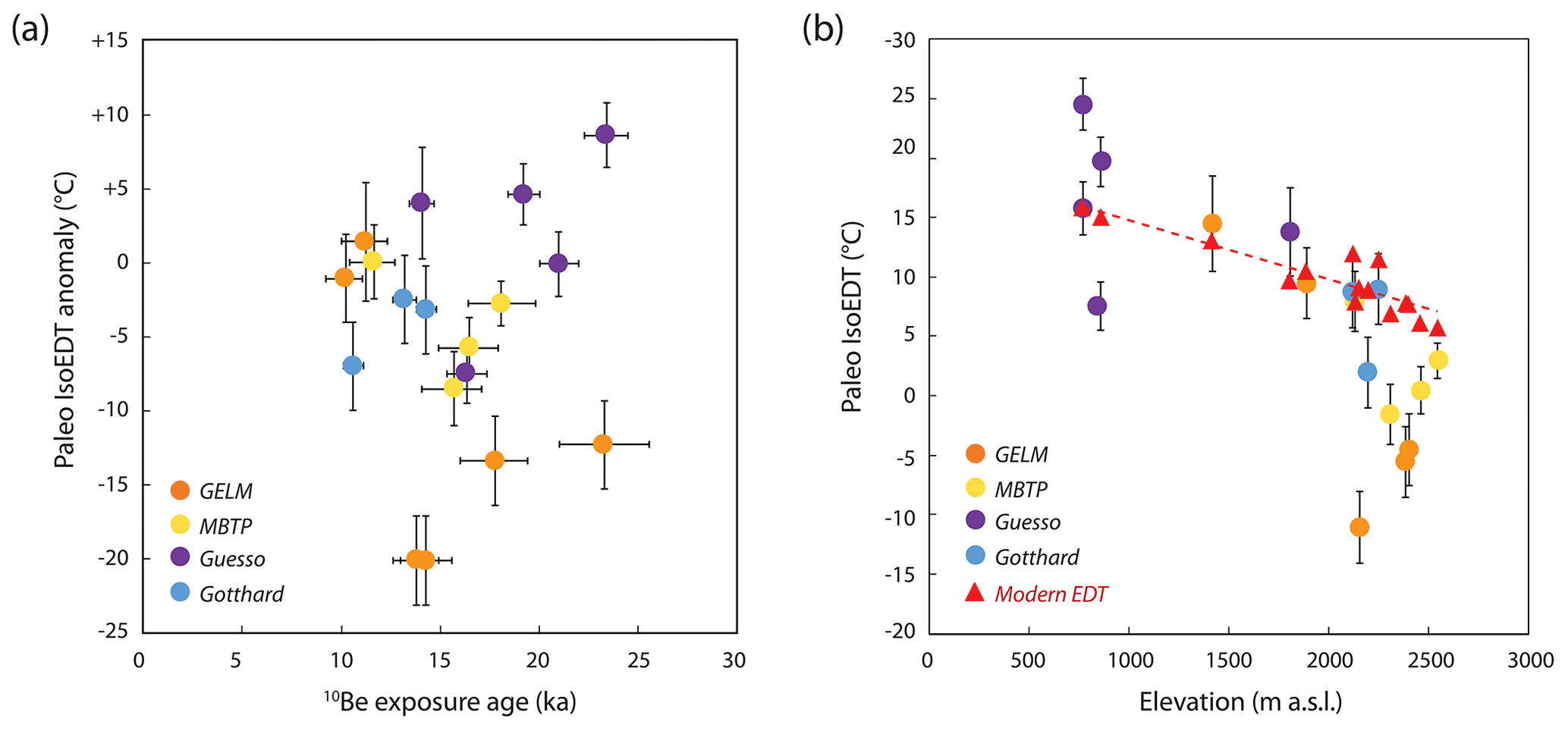
Figure 10(a) Relationship between 3He paleoIsoEDT anomaly and 10Be exposure age from available data from moraine boulders and glacially scoured bedrock surfaces in the Alps (results from this study; Tremblay et al., 2018, Gesso, and Guralnik et al., 2018, Gotthard). (b) Relationship between 3He paleoIsoEDT and elevation for same dataset as in panel (a).
Paleoglacier fluctuations in alpine settings lack direct constraints of associated past temperature and/or precipitation conditions, which are essential to improving our understanding of the response of glaciers and (para)glacial processes to past and future climate changes. In this study, we applied quartz 3He cosmogenic paleothermometry to derive in situ paleo-temperature (EDT) estimates along two deglaciation sequences gradually exposed from the Last Glacial Maximum to the Holocene in the western and northern European Alps (Mont Blanc and Aar massifs, MBTP and GELM, respectively). Investigation of quartz 3He diffusion kinetics indicates a clear difference between the two study sites, with quasi-linear vs. complex diffusion behaviors for MBTP and GELM sites, respectively. Based on the assumption that the same diffusion kinetics parameters apply to all samples at each site, forward numerical simulations of 3He production and diffusion suggest that no thermal signal from the Late Glacial period should be preserved in investigated rock surfaces with brief exposure durations (several kyr) before the transition to relatively stable Holocene climatic conditions like the present day. However, all our rock-surface samples exposed prior to Holocene indicate an apparent 3He thermal signal significantly colder than present-day conditions. Our recorded 3He signals cannot be explained by realistic post-LGM mean annual temperature evolution in the European Alps (as recorded by other paleoclimatic proxies), nor by changes in annual and/or diurnal temperature oscillations at the study sites.
When accounting for potential uncertainties related to Holocene thermal conditions and the quartz 3He production rate, the 3He signals (ΔEDT) recorded along the MBTP site can potentially be interpreted to be close to equilibrium with present-day and Holocene conditions, with minor change in mean annual temperature or diurnal and annual temperature oscillations. However, 3He-derived paleo-EDTs along the GELM site remain distinctively colder than present-day conditions. One hypothesis is that the multi-diffusion domain models applied to characterize the observed complex diffusion behavior in the GELM quartz do not accurately quantify quartz 3He diffusion for the samples of this site throughout their exposure histories. Alternatively, if the generally colder trend recorded along both profiles is possible, the assumed quartz 3He diffusion kinetics may inaccurately extrapolate to Earth surface temperatures, precluding quantitative EDT constraints from the observed 3He abundances in these samples. Finally, considering the high elevations of the investigated rock-surface samples (> 2000 m), it is also possible that our 3He thermal signals result from much more recent changes in Alpine permafrost ground conditions during the past decades and centuries. While the data presented in this study demonstrate the promising use of 3He cosmogenic paleothermometry to quantify past environmental changes, additional 3He analyses in high-alpine or cold settings would be necessary to clarify to which phenomena the 3He thermal signal is most responsive, i.e., between Late Pleistocene ambient temperature variations and recent changes in permafrost distribution.
The source codes used (1) to determine 3He diffusion kinetics from a step-heating experiment applying a MDD model framework and (2) to conduct forward simulation of 3He production and diffusion for a prescribed time–EDT scenario are available on Zenodo at https://doi.org/10.5281/zenodo.5808021 (Tremblay et al., 2021). The MDD code includes example stepwise-heating data from the experiment on MBT18-9, while the forward simulation code includes as an example a simplified LGM to present thermal history scenario for MBTP18-1.
No additional data are used in this paper that are not supplied in the Supplement.
The supplement related to this article is available online at: https://doi.org/10.5194/gchron-4-641-2022-supplement.
NG and PGV designed the study. NG led fieldwork campaigns with the support of BG and prepared samples for laboratory analysis. NG, GB, MMT, and DLS conducted the measurements. NG performed the numerical experiments using the model developed by MMT and GB. NG led the manuscript preparation, with contributions from all co-authors to the analysis and interpretation of the data, manuscript writing, and review.
At least one of the (co-)authors is a member of the editorial board of Geochronology. The peer-review process was guided by an independent editor, and the authors also have no other competing interests to declare.
Publisher's note: Copernicus Publications remains neutral with regard to jurisdictional claims in published maps and institutional affiliations.
This work was supported by the Swiss National Science Foundation (Grant no. PP00P2_170559), with measurements at BGC in part supported by the Ann and Gordon Getty Foundation. Pierre G. Valla acknowledges support from the French ANR-PIA program (ANR-18-MPGA-0006). Marissa M. Tremblay acknowledges support from the U.S. National Science Foundation (OPP-1935945) and the AAAS Marion Milligan Mason Fund. We thank Benjamin and Fred Lehmann and Guilhem A. Douillet for their help in the field when collecting samples. We thank Samuel Niedermann and two anonymous reviewers for their constructive comments that helped to improve this manuscript.
This research has been supported by the Schweizerischer Nationalfonds zur Förderung der Wissenschaftlichen Forschung (grant no. PP00P2_170559), the Agence Nationale de la Recherche (grant no. ANR-18-MPGA-0006), and the National Science Foundation (grant no. OPP-1935945).
This paper was edited by Klaus Mezger and reviewed by Samuel Niedermann and two anonymous referees.
Abrecht, J.: Geologic units of the Aar massif and their pre-Alpine rock associations: a critical review, Schweiz. Miner. Petrog., 74, 5–27, 1994.
Ackert, R. P., Mukhopadhyay, S., Pollard, D., DeConto, R. M., Putnam, A. E., and Borns, H. W.: West Antarctic Ice Sheet elevations in the Ohio Range: Geologic constraints and ice sheet modeling prior to the last highstand, Earth Planet. Sc. Lett., 307, 1–2, 83–93, https://doi.org/10.1016/j.epsl.2011.04.015, 2011.
Affolter, S., Häuselmann, A., Fleitmann, D., Lawrence Edwards, R., Cheng, H., and Leuenberger, M.: Central Europe temperature constrained by speleothem fluid inclusion water isotopes over the past 14,000 years, Science Advances, 5, eaav3809, https://doi.org/10.1126/sciadv.aav3809, 2019.
Allen, R., Siegert, M. J., and Payne, A. J.: Reconstructing glacier-based climates of LGM Europe and Russia – Part 2: A dataset of LGM precipitation/temperature relations derived from degree-day modelling of palaeo glaciers, Clim. Past, 4, 249–263, https://doi.org/10.5194/cp-4-249-2008, 2008.
André, M.-F.: Rates of postglacial rock weathering on glacially scoured outcrops (Abisko–Riksgränsen area, 68∘ N), Geogr. Ann. A, 84, 139–150, https://doi.org/10.1111/j.0435-3676.2002.00168.x, 2002.
Balco, G.: Contributions and unrealized potential contributions of cosmogenic-nuclide exposure dating to glacier chronology, 1990–2010, Quaternary Sci. Rev., 30, 3–27, https://doi.org/10.1016/j.quascirev.2010.11.003, 2011.
Balco, G., Stone, J. O., Lifton, N. A., and Dunai, T. J.: A complete and easily accessible means of calculating surface exposure ages or erosion rates from 10Be and 26Al measurements, Quat. Geochronol., 3, 174–195, https://doi.org/10.1016/j.quageo.2007.12.001, 2008.
Balco, G., Todd, C., Huybers, K., Campbell, S.., Vermeulen, M., Hegland, M., Goehring, B. M., and Hillebrand, T.: Cosmogenic-nuclide exposure ages from the Pensacola Mountains adjacent to the foundation ice stream, Antarctica, Am. J. Sci., 316, 542–577, https://doi.org/10.2475/06.2016.02, 2016.
Baroni, C., Gennaro, S., Cristina, M., Ivy-Ochs, S., Christl, M., Cerrato, R., and Orombelli, G.: Last Lateglacial glacier advance in the Gran Paradiso Group reveals relatively drier climatic conditions established in the Western Alps since at least the Younger Dryas, Quaternary Sci. Rev., 255, 106815, https://doi.org/10.1016/j.quascirev.2021.106815, 2021.
Bartlein, P. J., Harrison, S. P., Brewer, S., Connor, S., Davis, B. A. S., Gajewski, K., Guiot, J., Harrison-Prentice, T. I., Henderson, A., Peyron, O., Prentice, I. C., Scholze, M., Seppä, H., Shuman, B., Sugita, S., Thompson, R. S., Viau, E. A., Williams, J., and Wu, H.: Pollen-based continental climate reconstructions at 6 and 21 ka: a global synthesis, Clim. Dynam. 37, 775–802, https://doi.org/10.1007/s00382-010-0904-1, 2011.
Baxter, E. F.: Diffusion of noble gases in minerals, Rev. Mineral. Geochem., 72, 509–557, https://doi.org/10.2138/rmg.2010.72.11, 2010.
Becker, P., Seguinot, J., Jouvet, G., and Funk, M.: Last Glacial Maximum precipitation pattern in the Alps inferred from glacier modelling, Geogr. Helv., 71, 173–187, https://doi.org/10.5194/gh-71-173-2016, 2016.
Berger, G. W. and York, D.: Geothermometry from 40Ar/39Ar dating experiments, Geochim. Cosmochim. Ac., 45, 795–811, https://doi.org/10.1016/0016-7037(81)90109-5, 1981.
Beyerle, U., Purtschert, R., Aeschbach-Hertig, W., Imboden, D. M., Loosli, H. H., Wieler, R., and Kipfer, R.: Climate and Groundwater Recharge During the Last Glaciation in an Ice Covered Region, Science, 282, 731–734, https://doi.org/10.1126/science.282.5389.731, 1998.
Boeckli, L., Brenning, A., Gruber, S., and Noetzli, J.: A statistical approach to modelling permafrost distribution in the European Alps or similar mountain ranges, The Cryosphere, 6, 125–140, https://doi.org/10.5194/tc-6-125-2012, 2012a.
Boeckli, L., Brenning, A., Gruber, S., and Noetzli, J.: Permafrost distribution in the European Alps: calculation and evaluation of an index map and summary statistics, The Cryosphere, 6, 807–820, https://doi.org/10.5194/tc-6-807-2012, 2012b.
Borchers, B., Marrero, S. M., Balco, G., Caffee, M., Goehring, B., Lifton, N., Nishiizumi, K., Phillips, F. M., Schaefer, J., and Stone, J. O.: Geological calibration of spallation production rates in the CRONUS-Earth project, Quat. Geochronol., 31, 188–198, https://doi.org/10.1016/j.quageo.2015.01.009, 2016.
Brook, E. J. and Kurz, M. D.: Surface-exposure chronology using in situ cosmogenic 3He in antarctic quartz sandstone boulders, Quaternary Res., 39, 1–10, https://doi.org/10.1017/S0954102008001478, 1993.
Brook, E. J., Kurz, M. D., Ackert Jr., R. P., Denton, G. H., Brown, E. T., Raisbeck, G. M., and Yiou, F.: Chronology of glacier advances in Arena Valley, Antarctica, using in situ cosmogenic 3He and 10Be, Quaternary Res., 39, 11–23, https://doi.org/10.1006/qres.1993.1002, 1993.
Buizert, C., Keisling, B. A., Box, J. E., He, F., Carlson, A. E., Sinclair, G., and DeConto, R. M.: Greenland-wide seasonal temperatures during the last deglaciation, Geophys. Res. Lett., 45, 1905–1914, https://doi.org/10.1002/2017GL075601, 2018.
Cerling, T. E. and Craig, H.: Cosmogenic 3He production rates from 39∘ N to 46∘ N latitude, western USA and France, Geochim. Cosmochim. Ac., 58, 249–255, https://doi.org/10.1016/0016-7037(94)90462-6, 1994.
Christodoulides, C., Ettinger, K. V., and Fremlin, J. H.: The use of TL glow peaks at equilibrium in the examination of the thermal and radiation history of materials, Modern Geology, 2, 275–280, 1971.
Clark, P. U., Dyke, A. S., Shakun, J. D., Carlson, A. E., Clark, J., Wohlfarth, B., Mitrovica, J. X., Hostetler, S. W., and McCabe, A. M.: The Last Glacial Maximum, Science, 325, 710–714, https://doi.org/10.1126/science.1172873, 2009.
Clark, P. U., Shakun, J. D., Baker P. A., Bartlein, P. J., Brewer, S., Brook, E., Carlson, A. E., Cheng, H., Kaufman, D. S., Liu, Z., Marchitto, T. M., Mix, A. C., Morrill, C., Otto-Bliesner, B. L., Pahnk, K., Russell, J. M., Whitlock, C., Adkins, J. F., Blois, J. L., Clark, J., Colman, S. M., Curry, W. B., Flower, B. P., He, F., Johnson, T. C., Lynch-Stieglitz, J., Markgraf, V., McManus, J., Mitrovica, J. X., Moreno, P. I., and Williams, J. W.: Global climate evolution during the last deglaciation, P. Natl. Acad. Sci. USA, 109, 19, E1134–E1142, https://doi.org/10.1073/pnas.1116619109, 2012.
Cook, S. J., Swift, D. A., Kirkbride, M. P., Knight, P. G., and Waller, R. I.: The empirical basis for modelling glacial erosion rates, Nat. Commun., 11, 759, https://doi.org/10.1038/s41467-020-14583-8, 2020.
Davis, B. A. S., Brewer, S., Stevenson, A. C., Guiot, J., and Data contributors: The temperature of Europe during the Holocene reconstructed from pollen data, Quaternary Sci. Rev., 22, 1701–1716, https://doi.org/10.1016/S0277-3791(03)00173-2, 2003.
Dielforder, A. and Hetzel, R.: The deglaciation history of the Simplon region (southern Swiss Alps) constrained by 10Be exposure dating of ice-molded bedrock surfaces, Quaternary Sci. Rev., 84, 26–38, https://doi.org/10.1016/j.quascirev.2013.11.008, 2014.
Dobmeier, C.: Variscan P–T deformation paths from the southwestern Aiguilles Rouges massif (External massif, western Alps) and their implication for its tectonic evolution, Geol. Rundsch., 87, 107–123, https://doi.org/10.1007/s005310050193, 1998.
Domingos, R., Tremblay, M. M., Shuster, D. L., and Militzer, B.: Simulations and Experiments Reveal Effect of Nanopores on Helium Diffusion in Quartz, ACS Earth Space Chem., 4, 1906–1912, https://doi.org/10.1021/acsearthspacechem.0c00187, 2020.
Ehlers, J., Gibbard, P. L., and Hughes, P. D. (Eds.): Quaternary Glaciations – Extent and Chronology: A Closer Look, Developments in Quaternary Science, Vol. 15, Elsevier, Amsterdam, ISBN 978-0-444-53447-7, 2011.
Etzelmüller, B., Guglielmin, M., Hauck, C., Hilbich, C. Hoelzle, M., Isaksen, K., Noetzli, J., Oliva, M., and Ramos, M.: Twenty years of European mountain permafrost dynamics—the PACE legacy, Environ. Res. Lett., 15, 104070, https://doi.org/10.1088/1748-9326/abae9d, 2020.
Eynaud, F., de Abreu, L., Voelker, A., Schönfeld, J., Salgueiro, E., Turon, J-L., Penaud, A., Toucanne, S., Naughton F., Sanchez Goñi, M. F., Malizé, B., and Cacho, I.: Position of the Polar Front along the western Iberian margin during key cold episodes of the last 45 ka, Geochem. Geophy. Geosy., 10, Q07U05, https://doi.org/10.1029/2009GC002398, 2009.
Farley, K. A., Libarkin, J., Mukhopadhyay, S., and Amidon, W.: Cosmogenic and nucleogenic He-3 in apatite, titanite, and zircon, Earth Planet. Sc. Lett., 248, 451–461, https://doi.org/10.1016/j.epsl.2006.06.008, 2006.
Fechtig, H. and Kalbitzer, S.: The diffusion of argon in potassium-bearing solids, in: Potassium–Argon Dating, edited by: Schaeffer, O. A. and Zähringer, J., Springer, Heidelberg, https://doi.org/0.1007/978-3-642-87895-4_4, 1966.
Fick, S. E. and Hijmans, R. J.: WorldClim 2: new 1-km spatial resolution climate surfaces for global land areas, Int. J. Climatol., 37, 4302–4315, https://doi.org/10.1002/joc.5086, 2017.
Florineth, D. and Schlüchter, C.: Alpine evidence for atmospheric circulation patterns in Europe during the Last Glacial Maximum, Quaternary Res., 54, 295–308, https://doi.org/10.1006/qres.2000.2169, 2000.
Ghadiri, E., Vogel, N., Brennwald, M. S., Maden, C., Häuselmann, A. D., Fleitmann, D., Cheng, H., and Kipfer, R.: Noble gas-based temperature reconstruction on a Swiss stalagmite from the last glacial–interglacial transition and its comparison with other climate records, Earth Planet. Sc. Lett., 495, 192–201, https://doi.org/10.1016/j.epsl.2018.05.019, 2018.
Ghadiri, E., Affolter, S., Brennwald, M. S., Fleitmann, D., Häuselmann, A. D., Cheng, H., Maden, C., Leuenberger, M., and Kipfer, R.: Estimation of temperature – altitude gradients during the Pleistocene–Holocene transition from Swiss stalagmites, Earth Planet. Sc. Lett., 544, 116387, https://doi.org/10.1016/j.epsl.2020.116387, 2020.
Goehring, B. M., Kurz, M. D., Balco, G., Schaefer, J. M., Licciardi, J., and Lifton, N.: A reevaluation of in situ cosmogenic 3He production rates, Quat. Geochronol., 5, 410–418, https://doi.org/10.1016/j.quageo.2010.03.001, 2010.
Grämiger, L. M., Moore, J. R., Gischig, V. S., and Loew, S.: Thermomechanical stresses drive damage of Alpine valley rock walls during repeat glacial cycles, J. Geophys. Res.-Earth, 123, 2620–2646, https://doi.org/10.1029/2018JF004626, 2018.
Gribenski, N., Valla, P. G., Preusser, F., Roattino, T., Crouzet, C., and Buoncristiani, J.-F.: Out-of-phase Late Pleistocene glacial maxima in the Western Alps reflect past changes in North Atlantic atmospheric circulation, Geology, 49, 1096–1101, https://doi.org/10.1130/G48688.1, 2021.
Gruber, S., Peter, M., Hoelzle, M., Woodhatch, I., and Haeberli,W.: Surface temperatures in steep alpine rock faces: a strategy for regional-scale measurement and modelling, in: Proceedings of the 8th International Conference on Permafrost, Zurich, Switzerland, 21–25 July 2003, edited by: Arenson, L., Zürich, 325–330, ISBN-10: 9058096904, ISBN-13: 978-9058096906, 2003.
Gruber, S., Hoelzle, M., and Haeberli, W.: Rock-wall temperatures in the Alps: modelling their topographic distribution and regional differences, Permafrost Periglac., 15, 299–307, https://doi.org/10.1002/ppp.501, 2004.
Guralnik, B., Tremblay, M. M., Phillips, M., Gribenski, N., Valla, P., and Hippe, K.: Cosmogenic 3He-10Be-14C dating quantifies Alpine climate response to global warming, Goldschmidt Conference, Boston USA, 12–17 August 2018, Abstract no. 908, https://goldschmidtabstracts.info/2018/908.pdf (last access: 20 October 2022), 2018.
Haberkorn, A., Wever, N., Hoelzle, M., Phillips, M., Kenner, R., Bavay, M., and Lehning, M.: Distributed snow and rock temperature modelling in steep rock walls using Alpine3D, The Cryosphere, 11, 585–607, https://doi.org/10.5194/tc-11-585-2017, 2017.
Haeberli, W., Huggel, C., Paul, F., and Zemp, M.: 9.18 - The response of glaciers to climate change: observations and impacts, in: Treatise on Geomorphology, 2nd edn., edited by: Shroder, J. (J.) F., Academic Press, 404–439, ISBN 9780128182352, https://doi.org/10.1016/B978-0-12-818234-5.00011-0, 2022.
Hallet, B. A.: Theoretical Model of Glacial Abrasion, J. Glaciol., 23, 39–50, https://doi.org/10.3189/S0022143000029725, 1979.
Harrison, T. M. and Lovera, O. M.: The multi-diffusion domain model: past, present and future, Geological Society, London, Special Publications, 378, 91–106, https://doi.org/10.1144/SP378.9, 2013.
Harrison, T. M. and McDougall, I.: The thermal significance of potassium feldspar K–Ar ages inferred from 40Ar/39Ar age spectrum results, Geochim. Cosmochim. Ac., 46, 1811–1820, https://doi.org/10.1016/0016-7037(82)90120-X, 1982.
Hasler, A., Gruber, S., and Haeberli, W.: Temperature variability and offset in steep alpine rock and ice faces, The Cryosphere, 5, 977–988, https://doi.org/10.5194/tc-5-977-2011, 2011.
Heiri, O., Koinig, K. A., Spötl, C., Barrett, S., Brauer, A., Drescher-Schneider, R., Gaar, D., Ivy-Ochs, S., Kerschner, H., Luetscher, M., Moran, A., Nicolussi, K., Preusser, F., Schmidt, R., Schoeneich, P., Schwörer, C., Sprafke, T., Terhorst, B., and Tinner, W.: Palaeoclimate records 60–8 ka in the Austrian and Swiss Alps and their forelands, Quaternary Sci. Rev., 106, 186–205, https://doi.org/10.1016/j.quascirev.2014.05.021, 2014a.
Heiri, O., Brooks, S., Renssen, H., Bedford, A., Hazekamp, M., Ilyashuk, B., Jeffers, E. S., Lang, B., Kirilova, E., Kuiper, S., Millet, L., Samartin, S., Toth, M., Verbruggen, F., Watson, J., van Asch, N., Lammertsma, E., Amon, L., Birks, H. H., Birks, H. J. B., Mortensen, M. F., Hoek, W. Z., Magyari, E., Muñoz Sobrino, C., Seppä, H., Tinner, W., Tonkov, S., Vesli, S., and Lotter, A. F.: Validation of climate model-inferred regional temperature change for late-glacial Europe, Nat. Commun., 5, 1–7, https://doi.org/10.1038/ncomms5914, 2014b.
Herman, F., De Doncker, F., Delaney, I., Prasicek, G., and Koppes, M.: The impact of glaciers on mountain erosion, Nature Rev. Earth Environ., 2, 422–435, https://doi.org/10.1038/s43017-021-00165-9, 2021.
Ivy-Ochs, S.: Glacier variations in the European Alps at the end of the last glaciation, Cuad. Investig. Geografica, 41, 295–315, https://doi.org/10.18172/cig.2750, 2015.
Jaeger, J. M. and Koppes M. N.: The role of the cryosphere in source-to-sink systems, Earth-Sci. Rev., 153, 43–76, https://doi.org/10.1016/j.earscirev.2015.09.011, 2016.
Kalashnikov, E., Tolstikhin, I., Lehmann, B., and Pevzner, B.: Helium transport along lattice channels in crystalline quartz, J. Phys. Chem. Solids, 64, 2293–2300, https://doi.org/10.1016/S0022-3697(03)00264-6, 2003.
Kapannusch, R., Scherler, D., King G., and Wittmann, H.: Glacial influence on late Pleistocene 10Be-derived paleo-erosion rates in the north-western Himalaya, India, Earth Planet. Sc. Lett., 547, 116441, https://doi.org/10.1016/j.epsl.2020.116441, 2020.
Kelly, M. A., Ivy-Ochs, S., Kubik, P., von Blanckenburg, F., and Schlüchter, C.: Chronology of deglaciation based on 10Be dates of glacial erosional features in the Grimsel Pass region, central Swiss Alps, Boreas, 35, 634–643, https://doi.org/10.1080/03009480600690829, 2006.
Kerschner, H. and Ivy-Ochs, S.: Palaeoclimate from glaciers: examples from the Eastern Alps during the Alpine Lateglacial and early Holocene, Global Planet. Change, 60, 58–71, https://doi.org/10.1016/j.gloplacha.2006.07.034, 2008.
Kerschner, H., Kaser, G., and Sailer, R.: Alpine Younger Dryas glaciers as paleo-precipitation gauges, Ann. Glaciol., 31, 80–84, https://doi.org/10.3189/172756400781820237, 2000.
Koppes, M., Hallet, B., Rignot, E., Mouginot, J., Wellner, J. S., and Boldt, K.: Observed latitudinal variations in erosion as a function of glacier dynamics, Nature, 526, 100–103, https://doi.org/10.1038/nature15385, 2015.
Kuhlemann, J., Rohling, E. J., Krumrei, I., Kubik, I., Ivy-Ochs, S., Kucera, M.: Regional synthesis of Mediterranean atmospheric circulation during the Last Glacial Maximum, Science, 321, 1338–1340, https://doi.org/10.1126/science.1157638, 2008.
Labhart, T. P.: Aarmassiv und Gotthardmassiv, Gebrüder Borntraeger Verlagsbuchhandlung, Stuttgart, ISBN 10: 3443150195/ISBN 13: 9783443150198, 1977.
Lee, J. K. W.: Multipath diffusion in geochronology, Contrib. Mineral. Petr., 120, 60–82, https://doi.org/10.1007/BF00311008, 1995.
Lehmann, B., Herman, F., Valla, P. G., King, G. E., Biswas, R. H., Ivy-Ochs, S., Steinemann, O., and Christl, M.: Postglacial erosion of bedrock surfaces and deglaciation timing: New insights from the Mont Blanc massif (western Alps), Geology, 48, 139–144, https://doi.org/10.1130/G46585.1, 2020.
Li, H., Spötl, C., and Cheng, H.: A high-resolution speleothem proxy record of the Late Glacial in the European Alps: extending the NALPS19 record until the beginning of the Holocene, J. Quaternary Sci., 36, 29–39, https://doi.org/10.1002/jqs.3255, 2021.
Lin, K. J., Ding, H., and Demkowicz, M. J.: Formation, migration, and clustering energies of interstitial He in α-quartz and β-cristobalite, J. Nucl. Mater., 479, 224–231, https://doi.org/10.1016/j.jnucmat.2016.06.049, 2016.
Liu, H., Wang, L., Li, S., Yang, Y., Tian, H., Sun, F., Xu, C., Liu, L., Li, Y., Cui, Y., Li, Y., and Zhao, J.: A first-principles study of helium diffusion in quartz and coesite under high pressure up to 12 GPa, Geosci. Front., 12, 1001–1009, https://doi.org/10.1016/j.gsf.2020.09.009, 2021.
Lovera, O. M., Richter, F. M., and Harrison, T. M.: The 40Ar/39Ar thermochronometry for slowly cooled samples having a distribution of diffusion domain sizes, J. Geophys. Res., 94, 17917–17935, https://doi.org/10.1029/JB094iB12p17917, 1989.
Lovera, O. M., Richter, F. M., and Harrison, T. M.: Diffusion domains determined by 39Ar release during step heating, J. Geophys. Res., 96, 2057–2069, https://doi.org/10.1029/90JB02217, 1991.
Lovera, O. M., Grove, M., and Harrison, T. M.: Systematic analysis of K-feldspar 40Ar/39Ar step-heating experiments II: relevance of laboratory K-feldspar argon diffusion properties to Nature, Geochim. Cosmochim. Ac., 66, 1237–1255, https://doi.org/10.1016/S0016-7037(01)00846-8, 2002.
Luetscher, M., Boch, R., Sodemann, H., Spötl, C., Cheng, H., Edwards, R. L., Frisia, S., Hof, F., and Müller, W.: North Atlantic storm track changes during the Last Glacial Maximum recorded by Alpine speleothems, Nat. Commun., 6, 6344, https://doi.org/10.1038/ncomms7344, 2015.
Magnin, F., Brenning, A., Bodin, X., Deline, P., and Ravanel, L.: Statistical modelling of rock wall permafrost distribution: application to the Mont Blanc massif, Geomorphologie, 21, 145–162, https://doi.org/10.4000/geomorphologie.10965, 2015a.
Magnin, F., Deline, P., Ravanel, L., Noetzli, J., and Pogliotti, P.: Thermal characteristics of permafrost in the steep alpine rock walls of the Aiguille du Midi (Mont Blanc Massif, 3842 m a.s.l), The Cryosphere, 9, 109–121, https://doi.org/10.5194/tc-9-109-2015, 2015b.
Magnin, F., Josnin, J.-Y., Ravanel, L., Pergaud, J., Pohl, B., and Deline, P.: Modelling rock wall permafrost degradation in the Mont Blanc massif from the LIA to the end of the 21st century, The Cryosphere, 11, 1813–1834, https://doi.org/10.5194/tc-11-1813-2017, 2017.
Magny, M., Guiot, J., and Schoellammer, P.: Quantitative Reconstruction of Younger Dryas to Mid-Holocene Paleoclimates at Le Locle, Swiss Jura, Using Pollen and Lake-Level Data, Quaternary Res., 56, https://doi.org/10.1006/qres.2001.2257, 170–180, 2001.
Mair, D., Lechmann, A., Delunel, R., Yeşilyurt, S., Tikhomirov, D., Vockenhuber, C., Christl, M., Akçar, N., and Schlunegger, F.: The role of frost cracking in local denudation of steep Alpine rockwalls over millennia (Eiger, Switzerland), Earth Surf. Dynam., 8, 637–659, https://doi.org/10.5194/esurf-8-637-2020, 2020.
Mariotti, A., Blard, P.-H., Charreau, J., Toucanne, S., Jorry, S. J., Molliex, S., Bourlès, D. L., Aumaître, G., and Keddadouche, K.: Nonlinear forcing of climate on mountain denudation during glaciations, Nat. Geosci., 14, 16–22, https://doi.org/10.1038/s41561-020-00672-2, 2021.
Martin, L. C. P., Blard, P. H., Lavé, J., Jomelli, V., Charreau, J., Condom, T., Lupker, M., and ASTER Team: Antarctic-like temperature variations in the Tropical Andes recorded by glaciers and lakes during the last deglaciation, Quaternary Sci. Rev., 247, 106542, https://doi.org/10.1016/j.quascirev.2020.106542, 2020.
Masarik, J. and Reedy, R. C.: Terrestrial cosmogenic-nuclide production systematics calculated from numerical simulations, Earth Planet. Sc. Lett., 136, 381–395, https://doi.org/10.1016/0012-821X(95)00169-D, 1995.
Monegato, G., Scardia, G., Hajdas, I., Rizzini, F., and Piccin, A.: The Alpine LGM in the boreal ice-sheets game, Nature Sci. Reports, 7, 2078, https://doi.org/10.1038/s41598-017-02148-7, 2017.
Moseley, G. E., Spötl, C., Brandstätter, S., Erhardt, T., Luetscher, M., and Edwards, R. L.: NALPS19: sub-orbital-scale climate variability recorded in northern Alpine speleothems during the last glacial period, Clim. Past, 16, 29–50, https://doi.org/10.5194/cp-16-29-2020, 2020.
North Greenland Ice Core Project members: High-resolution record of Northern Hemisphere climate extending into the last interglacial period, Nature, 43, 147–151, https://doi.org/10.1038/nature02805, 2004.
Nichols, K. A. and Goehring, B. M.: Isolation of quartz for cosmogenic in situ 14C analysis, Geochronology, 1, 43–52, https://doi.org/10.5194/gchron-1-43-2019, 2019.
Niedermann, S: Cosmic-Ray-Produced Noble Gases in Terrestrial Rocks: Dating Tools for Surface Process, Rev. Mineral. Geochem., 47, 731–784, https://doi.org/10.2138/rmg.2002.47.16, 2002.
Peyron, O., Guiot, J., Cheddadi, R., Tarasov, P., Reille, M., de Beaulieu, J.-L., Bottema, S., and Andrieu, V.: Climatic Reconstruction in Europe for 18,000 YR B. P. from Pollen Data, Quaternary Res., 49, 183–196, https://doi.org/10.1006/qres.1997.1961, 1998.
Protin, M., Schimmelpfennig, I., Mugnier, J.-L., Ravanel, L., Le Roy, M., Deline, P., Favier, V., and Buoncristiani, J.-F.: Climatic reconstruction for the Younger Dryas/Early Holocene transition and the Little Ice Age based on paleo-extents of Argentière glacier (French Alps), Quaternary Sci. Rev., 221, 105863, https://doi.org/10.1016/j.quascirev.2019.105863, 2019.
Prud'homme, C., Vassallo, R., Crouzet, C., Cracaillet, J., Mugnier, J-L., and Cortès-Aranda, J.: Paired 10Be sampling of polished bedrock and erratic boulders to improve dating of glacial landforms: an example from the Western Alps, Earth Surf. Proc. Land., 45, 1168–1180, https://doi.org/10.1002/esp.4790, 2020.
Reddy, S. M., Potts, G. J., Kelley, S. P., and Arnaud, N. O.: The effects of deformation-induced microstructures on intragrain 40Ar/39Ar ages in potassium feldspar, Geology, 27, 363–366, https://doi.org/10.1130/0091-7613(1999)027<0363:TEODIM>2.3.CO;2, 1999.
Reiners, P. W., Ehlers, T. A., and Zeitler, P. K.: Past, Present, and Future of Thermochronology, Rev. Mineral. Geochem., 58, 1–18, https://doi.org/10.2138/rmg.2005.58.1, 2005.
Schaltegger, U. and Krähenbühl, U.: Heavy rare-earth element enrichment in granites of the Aar Massif (Central Alps, Switzerland), Chem. Geol., 89, 49–63, https://doi.org/10.1016/0009-2541(90)90059-G, 1990.
Seguinot, J., Ivy-Ochs, S., Jouvet, G., Huss, M., Funk, M., and Preusser, F.: Modelling last glacial cycle ice dynamics in the Alps, The Cryosphere, 12, 3265–3285, https://doi.org/10.5194/tc-12-3265-2018, 2018.
Seltzer, A. M., Ng, J., Aeschbach, W., Kipfer, R., Kulongoski, J. T., Severinghaus, J. P., and Stute, M.: Widespread six degrees Celsius cooling on land during the Last Glacial Maximum, Nature, 593, 228–232, https://doi.org/10.1038/s41586-021-03467-6, 2021.
Serra, E., Valla, P. G., Gribenski, N., Carcaillet, J., and Deline, P.: Post-LGM glacial and geomorphic evolution of the Dora Baltea valley (western Italian Alps), Quaternary Sci. Rev., 282, 107446, https://doi.org/10.1016/j.quascirev.2022.107446, 2022.
Shuster, D. L. and Farley, K. A.: Diffusion kinetics of proton induced 21Ne, 3He, and 4He in quartz, Geochim. Cosmochim. Ac., 69, 2349–2359, https://doi.org/10.1016/j.gca.2004.11.002, 2005.
Shuster, D. L., Farley, K. A., Sisterson, J. M., and Burnett D. S.: Quantifying the diffusion kinetics and spatial distributions of radiogenic 4He in minerals containing proton-induced 3He, Earth Planet. Sc. Lett., 217, 19–32, https://doi.org/10.1016/S0012-821X(03)00594-6, 2004.
Stone, J. O.: Air pressure and cosmogenic isotope production, J. Geophys. Res., 105, 753–759, https://doi.org/10.1029/2000JB900181, 2000.
Tremblay, M. M., Shuster D. L., and Balco, G.: Cosmogenic noble gas paleothermometry, Earth Planet. Sc. Lett., 400, 195–205, https://doi.org/10.1016/j.epsl.2014.05.040, 2014a.
Tremblay, M. M., Shuster, D. L., and Balco, G.: Diffusion Kinetics of 3He and 21Ne in Quartz and Implications for Cosmogenic Noble Gas Paleothermometry, Geochim. Cosmochim. Ac., 142, 186–204, https://doi.org/10.1016/j.gca.2014.08.010, 2014b.
Tremblay, M. M., Shuster, D., Spagnolo, M., Renssen, H., and Ribolini, A.: Temperatures recorded by cosmogenic noble gases since the last glacial maximum in the Maritime Alps, Quaternary Res., 91, 829–847, https://doi.org/10.1017/qua.2018.109, 2018.
Tremblay, M. M., Gribenski, N., Valla, P. G., Balco, G., Guralnik, B., and Shuster, D. L.: Thermochronology-At-Purdue/Gribenski2022: Gribenski2022_submissionv1.0.0 (v1.0.0), Zenodo [code], https://doi.org/10.5281/zenodo.5808021, 2021.
Vermeesch, P., Baur, H., Heber, V. S., Kober, F., Oberholzer, P., Schaefer, J. M., Schlüchter, C., Strasky, S., and Wieler, R.: Cosmogenic 3He and 21Ne measured in quartz targets after one year of exposure in the Swiss Alps, Earth Planet. Sc. Lett., 284, 417–425, https://doi.org/10.1016/j.epsl.2009.05.007, 2009.
Višnjević, V., Herman, F., and Prasicek, G.: Climatic patterns over the European Alps during the LGM derived from inversion of the paleo-ice extent, Earth Planet. Sc. Lett., 538, 116185, https://doi.org/10.1016/j.epsl.2020.116185, 2020.
Wirsig, C., Zasadni, J., Christl, M., Akçar, N., and Ivy-Ochs, S.: Dating the onset of LGM ice surface lowering in the High Alps, Quaternary Sci. Rev., 143, 37–50, https://doi.org/10.1016/j.quascirev.2016.05.001, 2016a.
Wirsig, C., Zasadni, J., Ivy-Ochs, S., Christl, M., Kober, F., and Schlüchter, C.: A deglaciation model of the Oberhasli, Switzerland, J. Quaternary Sci., 31, 46–59, https://doi.org/10.1002/jqs.2831, 2016b.
Wu, H. B., Guiot, J. L., Brewer, S., and Guo, Z. T.: Climatic changes in Eurasia and Africa at the last glacial maximum and mid-Holocene: reconstruction from pollen data using inverse vegetation modelling, Clim. Dynam., 29, 211–229, https://doi.org/10.1007/s00382-007-0231-3, 2007.
Zemp, M., Haeberli, W., Hoelzle, M., and Paul, F.: Alpine glaciers to disappear within decades?, Geophys. Res. Lett., 33, L13504, https://doi.org/10.1029/2006GL026319, 2006.