the Creative Commons Attribution 4.0 License.
the Creative Commons Attribution 4.0 License.
 | 03 Feb 2023
Bayesian age–depth modelling applied to varve and radiometric dating to optimize the transfer of an existing high-resolution chronology to a new composite sediment profile from Holzmaar (West Eifel Volcanic Field, Germany)
Wojciech Tylmann
Bernd Zolitschka
This study gives an overview of different methods to integrate information from a varve chronology and radiometric measurements in the Bayesian tool Bacon. These techniques will become important for the future as technologies evolve with more sites being revisited for the application of new and high-resolution scanning methods. Thus, the transfer of existing chronologies will become necessary because the recounting of varves will be too time consuming and expensive to be funded.
We introduce new sediment cores from Holzmaar (West Eifel Volcanic Field, Germany), a volcanic maar lake with a well-studied varve record. Four different age–depth models have been calculated for the new composite sediment profile (HZM19) using Bayesian modelling with Bacon. All models incorporate new Pb-210 and Cs-137 dates for the top of the record, the latest calibration curve (IntCal20) for radiocarbon ages as well as the new age estimation for the Laacher See Tephra. Model A is based on previously published radiocarbon measurements only, while Models B–D integrate the previously published varve chronology (VT-99) with different approaches. Model B rests upon radiocarbon data, while parameter settings are obtained from sedimentation rates derived from VT-99. Model C is based on radiocarbon dates and on VT-99 as several normal distributed tie points, while Model D is segmented into four sections: sections 1 and 3 are based on VT-99 only, whereas sections 2 and 4 rely on Bacon age–depth models including additional information from VT-99. In terms of accuracy, the parameter-based integration Model B shows little improvement over the non-integrated approach, whereas the tie-point-based integration Model C reflects the complex accumulation history of Holzmaar much better. Only the segmented and parameter-based age integration approach of Model D adapts and improves VT-99 by replacing sections of higher counting errors with Bayesian modelling of radiocarbon ages and thus efficiently makes available the best possible and most precise age–depth model for HZM19. This approach will value all ongoing high-resolution investigations for a better understanding of decadal-scale Holocene environmental and climatic variations.
- Article
(7933 KB) - Full-text XML
- BibTeX
- EndNote


Terrestrial archives from lakes have the potential to provide information about climate and the human history of its catchment area beyond instrumental and historical data (Berglund, 1986; Last and Smol, 2001a, b; Cohen, 2003). In the late 1980s, gravity coring (Kelts et al., 1986), piston coring (Nesje et al., 1987; Wright et al., 1984), and freeze coring techniques (Renberg and Hansson, 1993) for lacustrine sediment records improved tremendously, allowing a better quality of sediments to be recovered from modern lakes. Since then, the new fields of limnogeology and paleolimnology flourished alongside the increasing demand of societies for documentation of natural background data related to questions around acid rain (e.g. Battarbee et al., 1990), environmental pollution (e.g. Renberg et al., 1994), and a greater and greater focus on global climate change (e.g. Jenny et al., 2019).
To provide such information on not only local but also larger regional to global scales, investigations from different sites need to be compared and linked. However, such correlations are only successful if the contributing archives are based on robust chronologies. Therefore, precise and reliable age–depth models are the basis for sedimentary investigations and reconstructions of environmental and climatic changes of the past, as only they ensure intra-site comparability and enable recognition of larger scale patterns. A reliable chronology can be based on a combination of different dating techniques (multiple dating approach) such as radiometric dating, well-known events such as tephra layers (Turkey and Lowe, 2001; Davies, 2015), historic data (e.g. flood events), or varve counting. The term “varve” (Swedish for “layer”) was first introduced by De Geer (1912) for outcrops with proglacial sediments and describes finely laminated sediment structures with annual origin. The alternating pale and dark layers are driven by seasonal changes in temperature and precipitation that cause different chemical and biological processes within the lake and its catchment area. When anoxic conditions at the sediment–water interface are given at least seasonally, i.e. no bioturbation destroys laminations, varves are preserved and provide high-resolution and precise chronologies in calendar years (Zolitschka et al., 2015; Lamoureux, 2001).
Until the 1980s, varve chronologies were the only option for calendar year chronologies of sediment records, while AMS radiocarbon dating was still in its infancy and calibration of radiocarbon ages was restricted to tree rings of the middle and late Holocene (if applied at all; Pearson et al., 1977; Olsson, 1986). The first reviews about methodological advances in the study of annually laminated sediments appeared at the same time (Anderson and Dean, 1988; O'Sullivan, 1983; Saarnisto, 1986), and the first long and varve-dated reconstructions were published for Elk Lake, USA (Dean et al., 1984), and Lake Valkiajärvi, Finland (Saarnisto, 1985).
Meerfelder Maar and Holzmaar were the first varve-dated lacustrine records covering the entire Holocene and the Late Glacial for central Europe (Zolitschka, 1989, 1988), followed by records concentrating on the Late Glacial to Holocene transition at Soppensee, Switzerland (Lotter, 1991), and at Lake Gosciaz, Poland (Goslar et al., 1993). As such, the Holzmaar record became one of the best-studied lacustrine records in Europe (if not worldwide).
To produce the chronology for HZM19 we test and compare different methods integrating varve counts with radiometric measurements using Bayesian age–depth modelling. The advantage of any modelling approach is that all possible calendar ages of calibrated radiocarbon dates and their probability density functions (PDFs) will be tested by using a repeated random sampling method (Blaauw, 2010; Telford et al., 2004). In addition, using the Bayes theorem allows for the incorporation of information about the accumulation history known prior to modelling. Thus, calendar ages, which are monotonic with depth and have positive accumulation rates (in yr cm−1; in sedimentological terms, accumulation rates as they are used for Bayesian age–depth modelling are equivalent to “sedimentation rates”, as corroborated by the units used), are calculated (Lacourse and Gajewski, 2020; Trachsel and Telford, 2017). This is different and an advantage if compared to the “CLassical Age–depth Modelling” carried out by CLAM (Blaauw, 2010).
Currently established programs that use Bayesian statistics are OxCal (Bronk Ramsey, 2008), BChron (Haslett and Parnell, 2008), and Bacon (Blaauw and Christen, 2011), all of which differ in terms of parameter settings and handling of outliers. In this study, we focus on varve-counting integration methods using Bacon (rBacon version 2.5.7; Blaauw et al., 2021; Blaauw and Christen, 2011) for the R programming language (version 4.1.1; R Core Team, 2021), as it is one of the most often used software packages in paleo studies and provides many different ways for implementing additional information. Bacon uses a Markov chain Monte Carlo (MCMC) sampling strategy to model the accumulation history piecewise using a gamma autoregressive semi-parametric model (Blaauw and Christen, 2011). The accumulation rate of each segment depends on the accumulation rate of the previous segment. Dates are treated using a Student's t distribution. Although Bacon provides default values, the accumulation rate is controlled by two adjustable prior distributions (prior model), the accumulation rate as a gamma distribution and the memory, which describes the dependence of accumulation rates between neighbouring depths as a beta distribution. Both of the latter parameters are defined by a shape and a strength prior, respectively, in addition to a mean prior. Furthermore, we make use of the number of segments (thick parameter) recommended by Bacon. The program also allows for the incorporation of information about hiatus and slump events in the profile.
We concentrate on approaches using the Bacon package for the R statistical programming software (Blaauw and Christen, 2011), whereas the literature also provides comparable methods for alternative Bayesian age–depth modelling software, such as OxCal (Martin-Puertas et al., 2021; Bronk Ramsey, 2008; Vandergoes et al., 2018), which was also used to integrate varve counting and radiometric dating for the Holocene sediment record HZM96-4a/4b from Holzmaar (Prasad and Baier, 2014). As Bacon provides many different options to incorporate information into the age–depth model, in the literature only a few approaches are provided integrating varve and radiocarbon ages (Bonk et al., 2021; Vandergoes et al., 2018; Shanahan et al., 2012). For that reason, we summarize these approaches and compare them directly with each other. This will lead to faster decisions for future studies facing a comparable situation. As chronologies are always a “running target”, especially as new scientific methods and approaches appear, it is no wonder that the varve chronology for Holzmaar sediments has developed from its first attempt as “Varve Time 1990” (VT-90) (Zolitschka, 1990) to VT-99 10 years later (Zolitschka et al., 2000). In the course of applying ultra high-resolution (sub-millimetre-scale) scanning techniques to a new set of sediment cores from Holzmaar (HZM19), VT-99 is transferred to HZM19 making use of marker layers and radiocarbon ages for correlation and Bayesian age–depth modelling for the creation of an updated varve chronology (VT-22).
Different to earlier studies, we make use of available radiocarbon dates from Holzmaar not only to correct the varve chronology but to combine them with the independent radiocarbon chronology using Bayesian modelling. This integration approach is not commonly used for lacustrine records yet. Here we select three different methods to integrate varve and radiometric dating and apply them to the Holzmaar data. The aim of our study is to transfer and optimize the existing varve chronology from HZM-B/C to the new sediment record HZM19. In addition, we offer an overview about different approaches for age–depth modelling and their effects on model outcomes to researchers who face comparable challenges, thus supporting their decision making.
For this reason, we discuss the possibilities of integrating and improving the chronology by combining the varve chronology with modelling approaches using Bacon. This is accomplished by testing and comparing integration methods with regard to accuracy and precision obtained from the interpolated varve chronology itself and from a Bayesian model without any varve information relying on radiocarbon dates only. With this integration of all age information we produce the most reliable age estimations for the HZM19 record: VT-22. Based on the best model approach, this master chronology of VT-22 serves as the chronological backbone for ongoing and future biological, geochemical, and geophysical investigations conducted with the new Holzmaar sediment cores (e.g. García et al., 2022).
2.1 Regional settings
The late Quaternary volcanic maar lake Holzmaar (425 m a.s.l., 50∘7′8′′ N, 6∘52′45′′ E) is located in the western central part of the Rhenish Massif in the West Eifel Volcanic Field (WEVF; Rhineland-Palatinate, Germany, Fig. 1). The WEVF consists of more than 100 volcanic cones and maars, of which only 9 are water-filled examples today (Meyer, 2013; Schmincke, 2014). The volcanism in the Eifel region was caused by uplift of the Rhenish Shield since 700–800 ka, which started in the NW near Ormont (Meyer and Stets, 2002; Schmincke, 2007). Volcanic activities reached a peak at ca. 600–450 ka in the central WEVF and then decreased towards Bad Bertrich in the SE (Schmincke, 2007). The uplift is responsible for many eruptive centres at NW–SE-trending tectonic faults, along which several phreatomagmatic maar explosions occurred (Büchel, 1993; Lorenz, 1984; Lorenz et al., 2020; Meyer, 1985). One of these eruptions formed the Holzmaar system at ca. 40–70 ka (Büchel, 1993), consisting of three maars with the maar lake of Holzmaar, the raised bog of Dürres Maar, and the dry Hetsche or Hitsche Maar (from SE to NW). With 100 m in diameter, the latter is the smallest maar of the WEVF (Fig. 1).

Figure 1ESRI Satellite image of the Holzmaar volcanic system and its catchment area (indicated by a dashed white line) with Holzmaar, Dürres Maar, Hetsche Maar, and Sammetbach (blue line, flow direction indicated by arrows). The upper left insert shows the location of Holzmaar in Germany (red star). The upper right insert shows bathymetric map with isobaths in metres and coring locations (HZM19-07, -08, -10, and -11) marked by red stars.
The catchment area of Holzmaar (2.06 km2) includes the Sammetbach, a creek that flows in and out of the lake. Due to the low erosive energy of the stream, no delta formed in the lake (Scharf, 1987; Zolitschka, 1998a). The geology in the catchment area consists of Devonian metamorphic slates, greywackes, and quartzites in addition to Quaternary loess and volcanic rocks related to eruptions of the Holzmaar system (Meyer, 2013). Holzmaar has been located within a conservation area since 1975 protecting the surrounding beech forest (Fagus sylvatica L.), while ca. 60 % of the catchment area is in agricultural use (Kienel et al., 2005).
The lake of Holzmaar has a diameter of 300 m (water surface: 58 000 m2) and with a maximum water depth of 19–20 m shows a deep and steep-sided morphology typical for maar lakes. Only a small and shallow embayment in the SW interrupts the nearly circular and 1100 m long shoreline. This appendix-like bay developed due to an artificial damming in the late Middle Ages, which was constructed to supply a downstream water mill (Zolitschka, 1998a). For the last glacial, paleolimnological investigations indicate oligotrophic conditions, but eutrophication already started at the onset of the Late Glacial (García et al., 2022). During the Holocene, water quality was affected by human activities, which started during the Neolithic (around 6500 cal BP) according to pollen analysis (Litt et al., 2009). Together with the inflow of the Sammetbach this caused a steady but slow process of eutrophication and today leads to mesotrophic to eutrophic conditions (Lücke et al., 2003; Scharf and Oehms, 1992; Zolitschka, 1990). The lake is holomictic and dimictic with an anoxic hypolimnion during summer stratification (Scharf and Oehms, 1992). Altogether, this caused a high potential for varves to be formed and preserved.
2.2 Holzmaar lithology
In 2019 new sediment cores were retrieved from Holzmaar to compile the new record HZM19 (see Sect. 3.1, Fig. 2). The lithological description of HZM19 follows the characterization of Zolitschka (1998a, b), dividing the HZM84-B/C profile into 12 lithozones (H1–H12). We added the sediment colours found in HZM19 to this description.
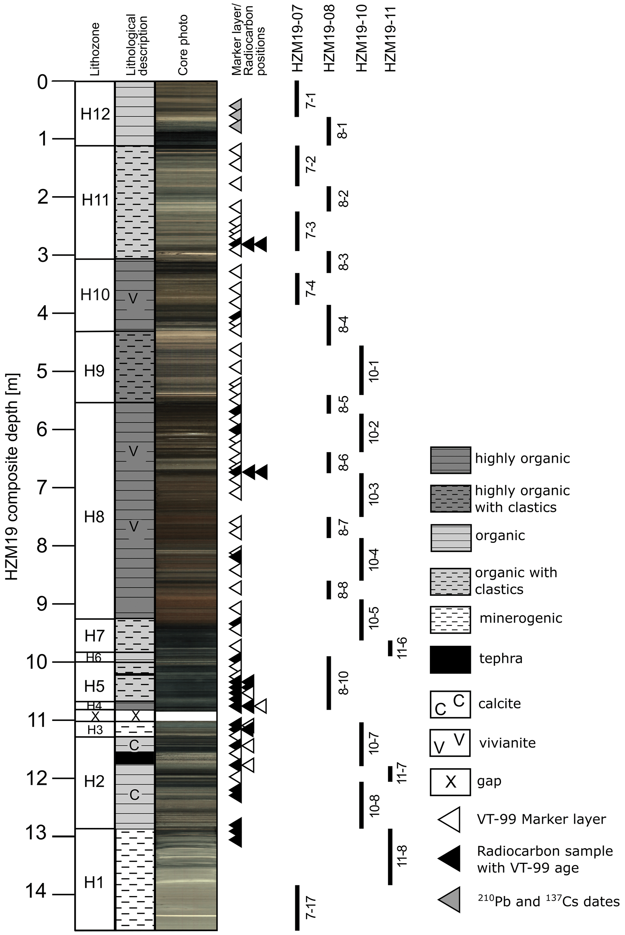
Figure 2Composite profile of HZM19 with (from left to right) lithozones H1 to H12 (see Table A1), lithological description, core photography taken immediately after core splitting, positions of marker layers and radiometric samples (see Tables A5 and A7), and core sections used for the composite profile (see Table A4).
Except H1, all lithozones cover finely laminated diatomaceous gyttja with varying minerogenic and organic content and colour. All lithozone depths are summarized in Table A1 in Appendix A. The transition from light greenish grey (10Y 8/1) and greyish brown (2.5Y 5/2) minerogenic, finely laminated, and weakly carbonaceous silts and clays in H1 (12.9–14.6 m) to carbonaceous laminated gyttja in light olive brown (2.5Y 5/3), black (10YR 2/1), and light-yellow brown (2.5Y 6/3) color with slightly higher organic content in H2 (11.3–12.9 m) indicates the transition from the Pleniglacial to the Late Glacial (Fig. 2).
Within H2, the distinct and almost 20 cm thick coarse-grained tephra from the Laacher See eruption (LST, 11.5–11.7 m) is deposited, which is a well-dated isochrone (Reinig et al., 2021) of European lake sediments (Fig. 2). The following lithozone H3 (10.9–11.3 m) shows a high minerogenic content and almost no organic components with colours of light greenish grey (5GY 7/1) and grey brown (10YR 5/2), representing the Younger Dryas (YD) at the end of the Pleistocene. Unfortunately, almost a third (12.9 cm) of the YD lithozone H3 is missing due to a technical gap (Fig. 2).
The Holocene sediment shows a periodic change from sections with higher organic content in black (2.5Y 2.5/1) and light olive brown (2.5Y 5/3) (H4: 10.7–10.9 m; H6: 9.9–10.0 m) to sections with high organic and clastic content in slightly brighter colours like grey (10YR 5/1) (H5: 10.0–10.7 m; H7: 9.3–9.9 m). The tephra of the Ulmener Maar eruption (UMT, ca. 3 mm thick) occurs in H5 at 10.24 m. The longest lithozone H8 (5.5–9.3 m) contains distinctly varved dark reddish brown (5YR 3/2) sediments with high organic content changing towards the top to very dark greyish brown (10YR 3/2) and brown (10YR 4/3) with several up to 5 mm thick lenses of authigenic vivianite. In addition, a low carbonate content was recognized. Furthermore, turbidites are observed more frequently from H8 to the top of HZM19 (Fig. 2).
Above H8, the clastic content increases and brightens up to light olive brown (2.5Y 5/3) and greyish brown (2.5Y 5/2) hues in H9 (4.3–5.5 m). In H10 (3.1–4.3 m) colours change to darker hues, e.g. olive grey (5Y 4/2) and black (5Y 2.5/2), while the organic content remains high and terrestrial macrofossils like pieces of wood or leaf remains occur more frequently towards the top. The organic content is decreasing slightly in H11 (1.1–3.1 m), which also contains clastic components and terrestrial plant material, as well as turbidites with paler colours, e.g. olive brown (2.5Y 5/3) and grey (2.5Y 5/1). The uppermost lithozone H12 (1.1 m to the top of HZM19) shows unconsolidated organic sediment with a homogenous blackish (5Y 2.5/1) colour for the lower part and brighter dark olive grey (5Y 3/2) sediment at the very top (Fig. 2).
2.3 Previous Holzmaar chronology
First varve counts and documentation of the annual origin for the finely laminated sediments preserved in the Holzmaar record were carried out in the late 1980s (Zolitschka, 1990, 1991, 1992), presenting the initial Holocene and Late Glacial varve chronology VT-90. Varve time (VT) refers to varve (calendar) years before 1950 CE (Common Era), which is equivalent to the commonly used reference timescale for radiocarbon dates provided in cal BP (calibrated years before present, i.e. 1950 CE). The chronology of VT-90 was elaborated for the HZM84-B/C composite record recovered in 1984 and was counted back to the onset of the Late Glacial, i.e. to 12 794 VT-90. This varve chronology was subsequently extended by counting the deeper, periglacial section back to the Last Glacial Maximum, i.e. to an age of 22 500 VT-90 (Brauer, 1994; Brauer et al., 1994).
By including the new sediment cores of HZM90-E/F/H, VT-90 was modified, resulting in VT-94. These overlapping sediment core series, as well as all other mentioned cores, have been recovered from the deepest part of Holzmaar, i.e. from within the 20 m isobath (Fig. 1). The recounting revealed an underestimation of the youngest 5000 years, for which 555 years have been added. This initial underestimation was mainly caused by sections with very thin varves being difficult to count (Zolitschka, 1998b). Another discrepancy occurred within the sediments of the YD, for which 245 years had to be added. Altogether, the difference from VT-90 to VT-94 comprises an addition of 800 years, shifting the basal age of the Late Glacial back to 13 594 VT-94 (Zolitschka, 1998b).
To crosscheck the varve chronology with an independent dating method, 41 samples of terrestrial macrofossils along the entire profile have been analysed using the AMS (accelerator mass spectrometry) radiocarbon method (Hajdas et al., 1995, and one unpublished radiocarbon date). A comparison between VT-94 and the calibrated radiocarbon chronology shows a discrepancy of +346 years between 3500 and 4500 VT-94 (Hajdas et al., 1995; Hajdas-Skowronek, 1993). This correction factor was estimated by χ2 minimization and added by linear interpolation between 3500 and 4500 VT-94. The outcome was VT-95, which consists of three segments. Segment I is covered by an “absolute” chronology until 3500 VT-95, while segment II (3500–4846 VT-95) was extended based on the discrepancy detected between varve and calibrated radiocarbon chronologies. Segment III covers sediments from 4846 to 13 940 VT-95 and is considered a floating chronology (Hajdas et al., 1995; Zolitschka, 1998b).
In 1996 new sediment cores (HZM96-4a/4b) have been obtained from Holzmaar and VT-95 was transferred to this new record using 26 distinct marker layers with their related VT and error. The age–depth model was subsequently obtained by linear interpolation (Baier et al., 2004). At the same time, novel varve counts for the Meerfelder Maar sediment record established 1880 varve years between the two isochrones of Laacher See Tephra (LST, eruption ca. 40 km NE from Holzmaar) and Ulmener Maar Tephra (UMT, eruption ca. 13 km NE from Holzmaar) (Brauer et al., 1999), which both are also archived in the Holzmaar sediment record. However, this well-constrained time interval was only 1560 years long for the Holzmaar record. The obviously missing 320 years have been positioned and added to VT-95 based on pollen data from Holzmaar (Leroy et al., 2000), assuming a hiatus for the middle part of the YD biozone at 12 025 VT-95. This resulted in the latest version (VT-99) of the Holzmaar varve chronology (Zolitschka et al., 2000) with a basal age of 14 260 VT-99 for the Late Glacial.
Varve quality and error estimations were first discussed and described based on multiple counts of selected and representative thin sections (Zolitschka, 1991). Later, different varve quality classes have been described in more detail for VT-90 (Zolitschka et al., 1992) and for VT-95 (Zolitschka, 1998b) with error estimations in the 1σ range (Table A2). Similar error margins were confirmed by counting more recent sediment profiles (HZM96-4a/4b) from Holzmaar (Prasad and Baier, 2014). In this study, the uppermost part was discussed as showing even higher counting uncertainties. However, no alternative error margins can be provided for this section. Thus, we use the data of Table A2 for further evaluations.
3.1 Sediment core collection
In August 2019, Holzmaar was revisited and four parallel cores (HZM19-07, HZM19-08, HZM19-10, HZM19-11) have been retrieved from the centre of the lake in 19 m water depth (Fig. 1) using a UWITEC piston corer with diameters of 90 mm (HZM19-07, -08, -10) and 60 mm (HZM19-11) from a coring platform. The coring locations are distributed evenly along a 12 m long transect with 4 to 4.4 m distance between coring locations. The recovered sediment cores have lengths of 2 m (HZM19-07, -08, -10) and 3 m (HZM19-11), which have been split in the field into 1 and 1.5 m long sections, respectively. In total, HZM19-07 covers a sediment depth of 15.5 m (0–15.5 m), while the other sites provided different depth ranges: HZM19-08 (0.25–10 m), HZM19-10 (4–14 m), and HZM19-11 (1–19 m). The water–sediment interface was perfectly recovered with HZM19-07-01 as the piston stopped 15 cm above the sediment surface. At the GEOPOLAR lab (University of Bremen) the cores have been split in halves lengthwise, photographed and visually described using a Munsell colour chart and according to the description guideline by Schnurrenberger et al. (2003). Cross correlation of all sediment core sections was conducted macroscopically using 48 distinct layers (Table A3).
The four parallel cores HZM19-07, -08, -10, and -11 were aligned and correlated to form the composite profile HZM19 (Fig. 2), which includes 24 core sections and reaches to a basal depth of 14.64 m (Table A4). One technical sediment gap exists at a composite depth of 10.90 m. To determine the precise length of this gap, we use core photography from a previous Holzmaar core (HZM90-H5u) and determined the technical gap to have a length of 12.9 cm (Fig. A1 in the Appendix).
3.2 Chronology
3.2.1 Pb-210 and Cs-137 dating
The isotopes Pb-210 and Cs-137 have been used to radiometrically date the uppermost part of HZM19 at the University of Gdańsk. In total, 61 samples were taken with a thickness of 2 cm. The activity of Cs-137 was determined directly by gamma-ray spectrometry from freeze-dried and homogenized samples. Gamma measurements were carried out using a HPGe well-type detector (GCW 2021) with a relative efficiency of 27 % and full width at half maximum (FWHM) of 1.9 at the energy of 1333 keV (Canberra). Energy and efficiency calibration were done using reference material CBSS-2 (Eurostandard CZ) in the same measurement geometry as the samples. The counting time for each sediment sample was 24 h.
Activity of total Pb-210 was determined indirectly by measuring Po-210 using alpha spectrometry. Dry and homogenized sediment samples of 0.2 g were spiked with a Po-209 yield tracer and digested with concentrated HNO3, HClO4, and HF at a temperature of 100 ∘C using a CEM Mars 6 microwave digestion system. The solution obtained was evaporated with 6 M HCl to dryness and then dissolved in 0.5 M HCl. Polonium isotopes were spontaneously deposited within 4 h on silver discs. Activities were measured using a 7200-04 APEX Alpha Analyst integrated alpha-spectroscopy system (Canberra) equipped with PIPS A450-18AM detectors. Samples were counted for 24 h. A certified mixed alpha source (U-234, U-238, Pu-239, and Am-241; SRS 73833-121, Analytics, Atlanta, USA) was used to check the detector counting efficiencies.
3.2.2 Bayesian age–depth modelling
Only few studies use the Bayesian approach that integrates varve counting information with radiocarbon dates (Bonk et al., 2021; Vandergoes et al., 2018; Shanahan et al., 2012; Fortin et al., 2019). We extracted three different methods and for comparison include one model only with radiocarbon data, i.e. excluding any VT-99 information. Thus, four different age–depth models (A–D) are presented in this study.
- A.
A model based only on radiocarbon dates is first discussed.
- B.
The parameter-based varve integration method introduced by Vandergoes et al. (2018) is then discussed, which compares several varve integration techniques for sediments from Lake Ohau (New Zealand) using both OxCal and Bacon. Here, we select the integration approach with Bacon, where the “varve counts function” is the source for the prior parameter of mean accumulation rate. Major changes in accumulation history recorded by the varve data are derived by using the R package “segmented” (Muggeo, 2022). It dissects the sediment sequence and for each resulting segment an individual mean accumulation rate prior is defined.
- C.
The tie-point-based integration used by Shanahan et al. (2012) is then discussed, which integrates the varve chronology from Lake Bosumtwi (Ghana) based on certain tie points with normally distributed age uncertainties of the cumulative error. They address the problem of integrating all individual varve counts, as they cannot be considered as independent chronological data points. Thus, they would be weighted too strongly in the model. The compromise they have chosen for this study is placing one varve tie point every 100 years. As there is no varve counting available for HZM19 but VT-99 ages based on marker layers, we implement them with cumulative errors as tie points instead.
- D.
The segmented and parameter-based integration introduced by Bonk et al. (2021) is the final method discussed and provides the most complex method for varve integration. The problem of not or poorly varved sections in the sediment profile of Lake Gosciaz (Poland) is compensated by dividing the profile into three sections and interpolating the section with low-quality varves using Bayesian modelling. For the Holzmaar record, we define four sections: sections 2 and 4 are based on Bayesian modelling, while sections 1 and 3 rely on VT-99. Section 3 is treated as a floating chronology and placed based on the sum of calibrated radiocarbon probabilities lying within this section. To tighten the two Bayesian modelled sections and the following varved sections, an anchor tie point based on the oldest age of the younger sections is implemented.
For each model we use radiocarbon dates published by Hajdas et al. (1995, 2000) (Table A5) and the calibration curve IntCal20 (Reimer et al., 2020) and make use of the default accumulation strength and memory priors. We also implement a surface age of cal BP as a tie point with a normal distributed error to anchor the chronology to present-day.
4.1 Transfer of VT-99 to HZM19
The varve chronology VT-99 (Zolitschka et al., 2000) was transferred to HZM19 by using 43 predefined marker layers and 41 radiocarbon sampling positions analysed by Hajdas et al. (1995, 2000) (Fig. A2) with their specific VT-99 ages and errors (Tables A2, A5). Both marker layers and radiocarbon sampling positions have been identified and justified by comparison with documents describing the samples as well as core photography from previous studies and sediment profiles, such as HZM90-E/F/H and HZM96-4a/4b. All marker layers cover an age range from 141 to 14 158 VT-99. After assignment, the ages of these marker layers have been linearly interpolated, and cumulative counting errors were calculated based on the 1σ errors provided with Table A2. All 84 marker layers distribute in HZM19 from 1.16 to 12.93 m and cover the entire VT-99 age range (Table A5). During the transfer of marker layers to HZM19 and comparison between HZM19 and previous Holzmaar sediment cores (HZM84-B/C, HZM92-E/-F/-H, HZM96-4a/4b), differences in position of the lowermost marker layers occurred (Fig. A2). All records show differences in distances between marker layers (ML) 1 (14 156 VT-99), ML-2 (14 152 VT-99), and ML-3 (13 646 VT-99), making a clear assignment of these layers difficult. Thus, we excluded these three marker layers for the transfer of VT-99 to HZM19. The lowermost applied marker layer is therefore ML-4, with a varve age of 13 087 VT-99 at a depth of 11.86 m. Because of inconsistencies in documentation, we excluded two more VT-99 ages, HZM-46 and HZM-10.1, i.e. those related to the radiocarbon ages (Table A5).
The marker layer density reaches a mean value of 5.5 dpm (dates per millennium), being most frequent before 10 000 and after 6000 cal BP (Fig. 3). We use a linear interpolation to receive an age–depth model based only on VT-99 with a resulting accuracy of 282 years as a mean age range and a maximum age range of 744 years (Table A6).
The radiocarbon dating density of HZM reaches an overall mean value of 2.7 dpm (Fig. 3), which is 35 % higher than the 2 dpm recommended for Bayesian modelling by Blaauw et al. (2018). However, their distribution is uneven. Radiocarbon dates are most frequent for ages > 10 000 cal BP with 3–7 dpm (mean: 5 dpm) (Fig. 3). A minimum density of radiocarbon dates (0–1 dpm) is obtained from 10 000 to 6000 cal BP (mean: 0.5 dpm). Therefore, a chronology based on the available radiocarbon data within this section should be interpreted with caution. Dating density for the uppermost 6000 years is higher and varies between 1 and 4 dpm (mean: 2.2 dpm).
When we compare VT-99 with radiocarbon ages calibrated with the latest calibration curve IntCal20 (Reimer et al., 2020), an overall agreement with marker layers is observed. Only for the lowermost part below approximately 10.64 m do we observe an increasing underestimation of VT-99 in relation to IntCal20-calibrated radiocarbon ages (Fig. A3, Table A5). This was already observed by Hajdas et al. (2000) in comparison to Intcal98 but has not been corrected yet.
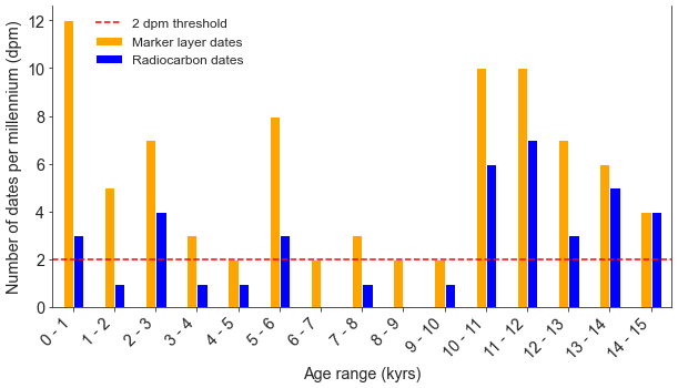
Figure 3Number of dating points per millennium (dpm) of HZM19 for marker layers (n: 84; mean: 5.5 dpm) and radiocarbon dates (n: 41; mean: 2.7 dpm). The dotted red line marks the recommended threshold of 2 dpm for Bayesian modelling suggested by Blaauw et al. (2018). Surface age and three ages estimated by Cs-137 are excluded.
4.2 Pb-210 and Cs-137 dating
The profile of unsupported Pb-210 activity concentration shows a gradual rather than an exponential decrease within the first metre of HZM19 (Fig. 4). Additionally, a plateau from 8 to 30 cm is interpreted as a section with rapid deposition of homogenous material and will be treated for further analyses as a slump event. Despite this irregularity, the gradual decrease in unsupported Pb-210 activity with depth indicates high sedimentation rates. We use the CFCS (constant flux and constant sedimentation) model to estimate mean sedimentation rates of 1.09±0.13 cm yr−1. This value should be treated with caution but suggests that the uppermost metre (including a 22 cm thick slump) was deposited over ca. 70 years.

Figure 4Results of unsupported Pb-210 (a) and Cs-137 (b) measurements with error bars for the uppermost 110 cm of HZM19. Shaded areas indicate the plateau shown by Pb-210 data, and black arrows mark peaks assigned to radiochronological events (given numbers are ages in years CE).
The variability in Cs-137 activity concentrations delivers three potential historical markers (Fig. 4). The Cs-137 profile is smooth, lacking sharp peaks due to high sedimentation rates and likely sediment focusing. The first traces of Cs-137 are recognizable at 101.2 cm and indicate atomic bomb testing in the early 1950s. At 89.2 cm, there is a significant increase signalling atmospheric fallout in the early 1960s in response to peak atomic bomb testing. Finally, at 69.2 cm a strong increase in Cs-137 documents the 1986 Chernobyl accident (Fig. 4, Table A7). This interpretation is generally in line with the results of Pb-210 dating. The shape of the Cs-137 record also corresponds nicely to the results of Sirocko et al. (2013), who measured Cs-137 on sediments from Schalkenmehrener Maar and Ulmener Maar (both in the WEVF). For both of these cases, the 1986 Chernobyl peak is also much larger than the one related to atomic bomb tests in 1963.
4.3 Age–depth modelling
Four different Bayesian age–depth models are calculated, of which three include varve ages (Models B–D) and one only radiocarbon ages (Model A). Common to all model runs are the default memory priors and the use of the IntCal20 calibration curve (Reimer et al., 2020). Furthermore, based on the Pb-210 and Cs-137 dating analysis, a slump at a composite depth of 8–30 cm was implemented. Another slump was assigned to a depth of 11.52–11.71 m at the isochrone of LST. As known from previous varve and pollen studies of the Holzmaar record (Brauer et al., 1999; Leroy et al., 2000), 320 years are missing during the YD and have been included into VT-99 at 12 025 VT-99. Based on the study of Leroy et al. (2000), we were able to locate the position of the YD hiatus to a depth of 11.09 m, which we implemented for each model with a maximum duration of 320 years. In addition to marker layers and radiocarbon dates, we included the surface age of cal BP and three events dated by Cs-137 (Table A7).
Preliminary test runs reveal two necessary changes to be made for the calculations. (1) The default number of iterations is too low to produce a robust model for the entire HZM19 sediment sequence. Thus, we use the Baconvergence() function of Bacon to estimate the number of iterations needed. This function repeats the calculations and tests if the MCMC mixing of the core results in a robust model by calculating the “Gelman and Rubin Reduction Factor” (Brooks and Gelman, 1998). Good mixing is indicated by a threshold of <1.05, which in our case was reached after three repetitions when the number of iterations was increased to 40 000. This results in a better mix of MCMC iterations but also in long calculation times (>5 h). (2) For each test run, Bacon predicted ages that were consistently too old for the LST, which is probably caused by the slightly too old ages of the surrounding radiocarbon dates (Table A5). To gain a better comparability with studies from other sites, we decided to include the latest LST age of 13 006 ± 9 cal BP (Reinig et al., 2021, Table A7).
In addition, we extended the age–depth model to a maximum depth of 14.64 m, as ongoing analyses exceed the lowermost dated level. However, in the following sections we only discuss the model output between the first (ML36/1) and the last (HZM-19) marker layer at 12.93 m (Table A5) and compare it with the interpolated varve chronology (VT-99).
After each calculation and if the Bacon output indicates a highly variable log of objectives or MCMC iterations, we made use of the scissor() command to achieve a better mixing of the output. All Bacon model outputs with their settings and additional information are shown in Fig. 5, and related ages are listed in Table A6.
The model without varve integration (Model A) is based on the year of sediment recovery (surface age), three dates estimated by Cs-137 analyses, the age for the LST (Reinig et al., 2021) and 41 calibrated radiocarbon probability density functions (Fig. 5a). Different to Hajdas et al. (1995), this model includes the outlier of HZM-23 but excludes HZM-24 and other described outliers (Table A5).
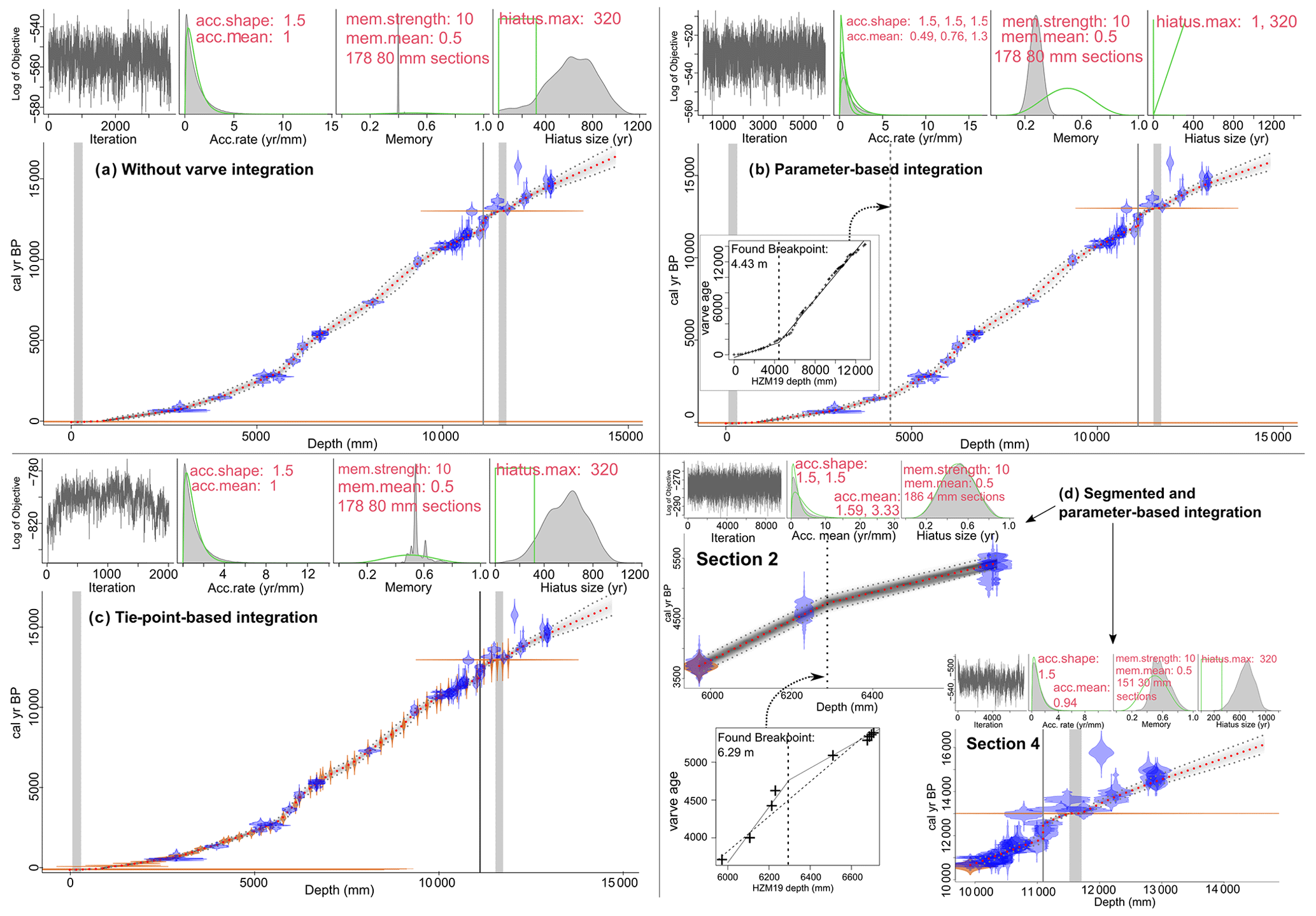
Figure 5Bacon output for Models A (a), B (b), C (c), and D (d) (sections 2 and 4). In each age-depth model plot (a–d): MCMC iterations, prior (green) and posterior (grey) for accumulation rate distribution, memory, and hiatus with defined settings in red. The main graph in each age–depth model plot shows the model with calibrated radiocarbon date probabilities (blue), tie points with normal distribution (orange), and the posterior age–depth model with mean (dotted red line) and 95 % confidence intervals (dotted grey line). The vertical grey lines (from left to right) in the main graphs show the slump event, defined hiatus, and Laacher See Tephra. Two boundaries indicating major changes in accumulation rate are provided as vertical dotted lines.
Model A results in an age of 14 615 cal BP [14 339, 14 926] at the lowermost dated depth of 12.93 m with a mean age uncertainty of 468 years. The maximum age uncertainty of approx. 1056 years occurs at a depth of 8.86 m within lithozone H8 (Table A6), where radiocarbon dating density is <1 dpm (Fig. 3).
The parameter-based integration (Model B) integrates VT-99 using all dates as in Model A and adjusts the prior information given for the calculation based on the varve accumulation history. We follow the procedure presented by Vandergoes et al. (2018) and calculate a breakpoint based on ages and depths of the marker layers at 4.43 m, i.e. at 1312 VT-99 (Fig. 5b). This boundary is implemented as an additional hiatus to the Bacon code with a duration of 1 year. The accumulation rate prior is set based on published sedimentation rates (Zolitschka et al., 2000). We calculate with a mean of 0.49 yr mm−1 for the uppermost part (−9 to 1312 VT-99), with 1.30 yr mm−1 from 1312 to the YD hiatus at 12 025 VT-99 and with 0.76 yr mm−1 from the YD hiatus to the lowermost age of 14 158 VT-99. Model B is calculated using the same parameters as for Model A and with the same treatment of outliers.
The resulting posterior model shows similarities to Model A, having a maximum mean age of 14 456 cal BP [14 236, 14 749] at a depth of 12.93 m and a mean 95 % confidence interval of 456 years with a maximum of 1064 years at 8.78 m, i.e. within the period of lowest radiocarbon dating density (Fig. 3).
The tie-point-based integration (Model C) is based on the approach used by Shanahan et al. (2012). We include 43 marker layers with related VT-99 ages and cumulative errors as normal distributed tie points into the model, which adds to the dates used in Models A and B and sums up to 89 dates. This approach increases the amount of chronological information and fills areas with larger gaps between radiocarbon dates. The model was run with default settings provided by Bacon (Fig. 5c). Bacon recognizes the outliers in the same way as by previously described models.
Model C results in a maximum age of 14 614 cal BP [14 332, 14 919] (at 12.93 m) with a mean 95 % confidence interval of 329 years, which is better than for Models A and B. A maximum age range of 749 years is given at a depth of 9.18 m, which is also slightly better than for previously presented models. However, Model C produced the MCMC iterations with the highest noise, and it was therefore difficult to cut out a well-mixed section (Fig. 5c, upper left).
The segmented and parameter-based integration (Model D) is a more complex method of varve integration used by Bonk et al. (2021) and was adapted for the HZM19 profile by dividing the varve chronology of VT-99 into four sections. This separation is based on variations in counting uncertainty and radiocarbon sampling density and an increasing offset of VT-99 to the latest calibration curve IntCal20 (Fig. A3).
Section 1 (0–5.98 m) and section 3 (6.70–9.90 m) are transferred and interpolated based on VT-99 marker layers, as they are consistent with calibrated radiocarbon data (section 1) and have well-preserved varves with small counting errors of ±0.7 % (section 3). Section 2 (5.98–6.70 m) and section 4 (9.90–14.60 m) are reported as showing higher counting uncertainties (section 2) or increasing differences between VT-99 and the calibration curve (section 4). Thus, we replace the varve chronology in sections 2 and 4 with Bayesian age–depth modelling (Fig. 5d). Section 4 also contains very dense radiocarbon dates (Hajdas et al., 2000), which increase the predictability of Bacon (Fig. 3).
Section 1 is based on linear interpolation for ages of the sediment surface ( cal BP), three dates derived by Cs-137 analyses (Table A7), and 25 ages of marker layers with a basal age of 3704±134 cal BP at the position of HZM-25 (Table A5).
The modelled section 2, previously identified as a section with sedimentation rates >2.86 yr mm−1 and therefore a source of high counting uncertainties and underestimation of varve ages (Zolitschka et al., 2000), consists of five radiocarbon dates (Table A5) and the basal age of section 1 (3704±134 cal BP) as anchor point for section 2. To reduce the resulting gap between sections 1 and 2, we reduce the error estimation for the anchor point to ±70 years (±0.5σ). As there is a major change in sedimentation rates within this section, we calculated a boundary similar to that in Model B using the marker layers of this section (Fig. 5d). This allows for defining a boundary at the depth of 6.29 m with adjusted accumulation means of 3.33 yr mm−1 above (5.98–6.29 m) and 1.59 yr mm−1 below (6.29–6.70 m) using published sedimentation rate data (Zolitschka et al., 2000). Based on suggestions by the software, the “thick” parameter was set to 4 mm. The resulting model covers and age range from 3709 [3591, 3825] to 5419 cal BP [5329, 5548] (Fig. 5d, section 2).
Section 3 interpolates 16 marker layers (Table A5), which are treated as a floating chronology. The placement of the anchor point relates to the basal age of the lowermost calibrated radiocarbon date (HZM-4.3) in section 2 (Table A5) and the maximum sum of the four calibrated radiocarbon PDFs within this part, with a summed probability of 0.076 at 5450±165 cal BP (Fig. A4a).
In comparison to the original VT-99, this approach results in a shift of +65 years for all marker layers within section 3 (Fig. A4b). Thus, a basal age of 10 619 ± 213 cal BP is obtained for section 3.
The basal age of section 3 is implemented as the anchor tie point for the Bacon calculation of section 4 with a reduced error of 100 years to bring both sections closer to each other. In addition to the difficulties based on missing sediment within the YD, this section is the source of the highest counting uncertainties for VT-99. Section 4 is based on 25 radiocarbon dates and the latest age estimation for the LST (Table A5). As in section 2, we adjusted the sedimentation rate prior (= 0.94 yr mm−1) based on VT-99 accumulation rate data (Zolitschka et al., 2000). The Bacon software suggests a segment length of 30 mm that we applied. The resulting model covers an age range from 10 663 [10 457, 10 864] to 14 485 cal BP [14 287, 14 721] at 12.93 m (Fig. 5d, section 4).
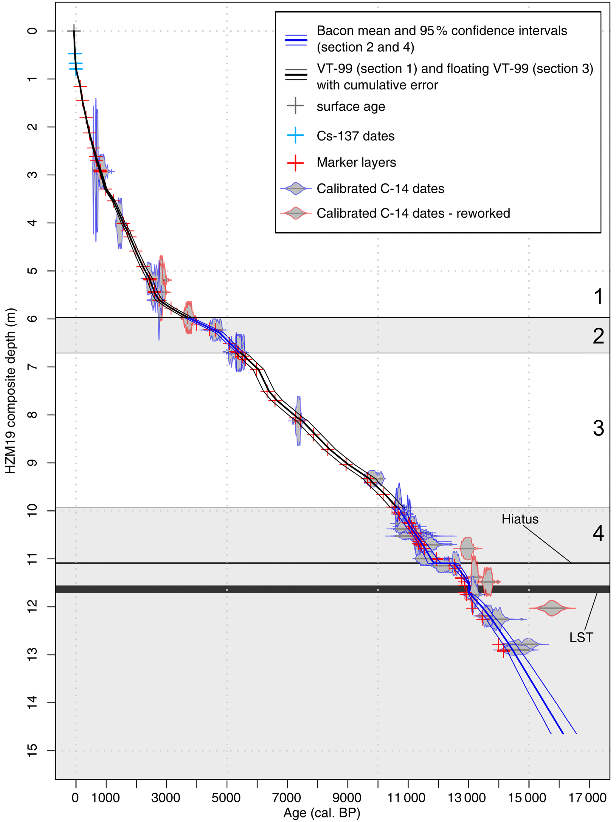
Figure 6Age–depth model for HZM19 based on Model D, with sections 1 and 3 based on VT-99 (section numbers at the right) and sections 2 and 4 based on Bayesian modelling (shaded).
If all sections are merged, the continuous age–depth relationship forming Model D (Fig. 6) consists of 63 % VT-99 ages and 37 % Bacon-modelled ages with 80 missing years in total between the sections, as it is not possible to determine the exact start and end ages of the models. This segmented and parameter-based integration model results in a maximum age of 14 485 cal BP [14 287, 14 721] (at 12.93 m) with a mean age uncertainty of 229 years, which is the smallest of all four tested models. The maximum age range is 447 years at 11.09 m depth, and it is thus considerably smaller compared to those of Models A to C (Table A6).
4.4 Comparison of model output with VT-99
The comparison of all presented models differs in terms of the means and accuracies of predicted ages along the core (Fig. 7a1; b1; c1; d1), which becomes more evident in comparison with VT-99 (Fig. 7a2, 3; b2, 3; c2, 3; d2, 3). These differences in mean modelled age and mean VT-99 age vary in direction and amplitude (Fig. 7a2; b2; c2; d2). The largest age differences during the Holocene occur in Model A and B with up to 300 years between 4 and 6 m depth (Fig. 7a2; b2). The defined boundary in Model B results in large differences within the boundary area, predicting much younger ages than VT-99. Due to the small cumulative counting uncertainty of VT-99 in the upper part of the profile, the mean of Model B outranges the VT-99 error in most sections above 6 m (Fig. 7b2).
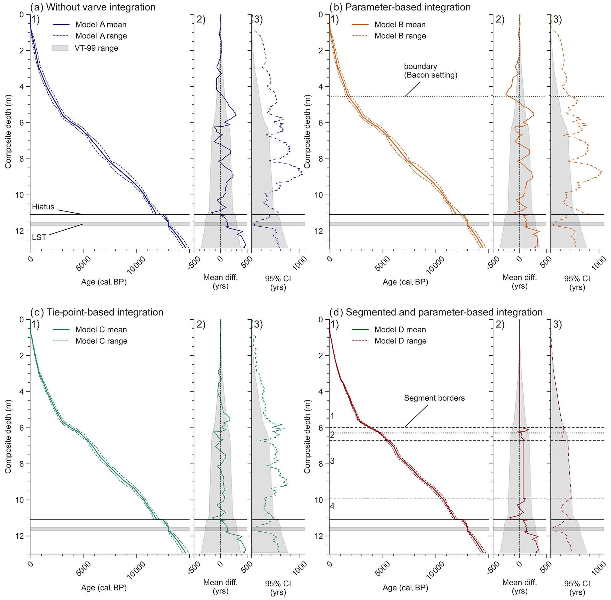
Figure 7Results of Models A (a), B (b), C (c), and D (d) plotted against composite depth (1), compared to VT-99 as the difference in mean ages (model mean–VT-99 mean) (2), and plotted vs. VT-99 confidence intervals (CIs) (3).
The approach used for Model C reduces the difference between VT-99 and the model, which is probably a result of increased dating density (Fig. 7c2). This approach also leads to less overestimations and underestimations of the model's mean age and the VT-99 age range (Fig. 7c2). Only the segmented insertion of VT-99 in Model D results in comparable ages during the Holocene (Fig. 7d2)
In the Late Glacial component below 11 m, all models produce ages that are constantly older than VT-99 (Fig. 7a2, b2, c2, d2). The age differences are even higher (up to 477 years) when the Bacon prior for accumulation rates was not adjusted to VT-99 (Fig. 7a2, c2). In the other cases the maximum age differences are 369 and 354 years for Model B and Model D, respectively (Fig. 7b2, d2). Hajdas et al. (2000) already observed a shift between the varve ages of radiocarbon-dated samples and calibrated ages using the INTCAL98 calibration curve (Stuiver et al., 1998) and discuss the difference using the LST age estimation from Meerfelder Maar (12 880 VT). However, no adjustment has been made to fit the VT-99 ages to the calibration curve. With the LST dated to 13 006 ± 9 cal BP (Reinig et al., 2021) and the use of the INTCAL20 calibration curve, an underestimation of VT-99 compared to the calibration curve still exists (Fig. A3). Therefore, a correction of ages older than 12 800 cal BP is needed to ensure comparability of HZM19 to other sites.
In order to find the best method to transfer VT-99 to HZM19 and to improve the chronology by using Bayesian modelling, a closer look at each model's accuracy is necessary (Fig. 7a3, b3, c3, d3). In comparison to the cumulative VT-99 counting error, Models A and B show maximum differences in age uncertainties of up to +655 and +665 years, respectively (Table A6). Both models predict ages with larger uncertainties than the estimated counting error for VT-99, especially above 9.82 m and particularly with increasing distance to radiocarbon-dated levels. Therefore, no improvement in the accuracy of age estimations is observed when using the parameter-based approach (Model B).
The tie-point-based Model C also predicts larger uncertainties than VT-99 above 9.82 m (Fig. 7c), whereas the overall difference in the age range is reduced to a mean of 47 years with a maximum of +401 years (Table A6). Only the segmented and parameter-based Model D shows no significantly enlarged age uncertainties and an overall improved mean age range as it adapts the cumulative error of the varve chronology in sections 1 and 3 (Table A6). The overall improvement occurs in sections 2 and 4, which is the result of more detailed prior settings for the model run. However, all age models result in more accurate age estimations in the Late Glacial part, where the cumulative counting error is higher and radiocarbon dating sampling is dense. However, we still see that Models C and D perform best within this section, as they predict ages with constantly lower uncertainty ranges than VT-99. This is in contrast to the other models, which show increased and therefore larger uncertainties at a depth of ca. 11 m. As we calculate this section in Model D with the same data as for Models A and B, we assume that the better adjustment of the sedimentation rate mean prior of Model D influences the model's accuracy. In terms of accuracy, there are no general improvements in calculating a single model for the entire record, but improvements are realized by adjusting the priors in a more detailed way.
4.5 Comparison of model output with common isochrones
The tephra layers of UMT and LST have been identified for sediments from Holzmaar and Meerfelder Maar (Brauer et al., 1999). The varve age of 11 000 VT-99 for UMT was derived from the Holzmaar chronology (Zolitschka, 1998b), while the YD hiatus of this site did not allow any calendar year estimation for LST. As no such hiatus exists between these two isochrones at Meerfelder Maar, the age for the LST was derived as 1880 varve years older than UMT, i.e. as 12 880 VT-99. A recent study presents a new age for the LST that is 126 years older (Reinig et al., 2021). This age of 13 006 cal BP was implemented for the calculation of Models A–D.
When we compare all models, the age estimations for UMT are close to the published ages, with the UMT dated ca. 20–50 years earlier, and thus match well within the 95 % confidence interval (Fig. A5, Table A6). Due to the new age of LST, the distances between both isochrones vary from 2030 (Model D) to 2057 years (Model C), which is 150–177 years more than for Meerfelder Maar (Fig. A5).
The main differences occur in the prediction of the end of the YD that defines the transition to the Holocene. The rapid cooling and subsequent warming left behind easy to recognize traces in many European lake records, increasing the comparability between sites. The entire YD is not covered by HZM19 due to a technical gap. Nevertheless, we are able to estimate depth and time range based on detailed pollen investigations (Leroy et al., 2000). Using VT-99, Leroy et al. (2000) date the onset of the YD, i.e. the Allerød–Younger Dryas transition (AL/YD), to 12 606 VT-99 and the Younger Dryas–Preboreal (YD/PB) transition to 11 632 VT-99, with a 320-year hiatus at 12 025 VT-99. For HZM19 these boundaries occur at 10.88 m (YD/PB) and at 11.26 m (AL/YD) with the hiatus found at 11.11 m (Figs. 7, A5).
All model runs predict a YD duration in the range of 1012 (Model C) to 1073 (Model D) years, which is longer than the 974 years given by VT-99 (Fig. A5, Table A6). However, the predicted times are closer to the duration counted for Meerfelder Maar (1080 years) (Brauer et al., 1999) or the even longer time span detected for Lake Gosciaz (1150 years) (Bonk et al., 2021).
Moreover, the onset and end of the YD have been predicted within the 95 % confidence interval comparable to VT-99 (Fig. A5, Table A6) and to the Meerfelder Maar record. Only the AL/YD transition varies between 12 694 (Model C) and 12 737 cal BP (Model B) and is thus predicted earlier than for VT-99 (12 606 VT-99). However, this age range still covers the age estimations from Lake Gosciaz (12 620 cal BP [12 389, 12 753]) and Meerfelder Maar (12 680 cal BP [12 640, 12 720]) (Fig. A5). In contrast, the YD/PB transition varies between 11 655 (Model D) and 11 723 cal BP (Model B), which is slightly earlier than estimated by Meerfelder Maar (11 600 cal BP [11 570, 11 630]) and much earlier than the age estimation for Lake Gosciaz (11 470 cal BP [11 264, 11 596]) (Fig. A5). These discrepancies between the boundaries of the YD biozone obtained by VT-99 and those obtained by the model runs are probably related to the new and 126-year-older age for the LST, which is included with all models. Thus, age discrepancies are attenuating towards the UMT with 110 years at the AL/YD transition and 57 years at the YD/PB transition (Fig. A5).
All models predict convincing age estimations for the isochrones of UMT, whereas the prediction of the YD between both isochrones remains somewhat ambiguous due to a documented hiatus and too few radiocarbon ages being available for this biozone.
In terms of accuracy and precision, the varve integration technique applied in Model D and introduced by Bonk et al. (2021) results in the most convincing age estimations for HZM19. Especially in terms of accuracy, none of the completely Bayesian-modelled age–depth relationships improved the small age uncertainties in VT-99 in the upper part. Only in sections with markedly higher radiocarbon sampling density or in sections with high varve counting uncertainty did the Bacon models perform better and result in more accurate age estimations than VT-99.
In comparison, Model B shows nearly no improvement over the approach without varve integration (Model A). The reason is probably the low-resolution definition of sedimentation rate changes (boundaries) for HZM19, which does not reflect the complex accumulation history. Vandergoes et al. (2018) also reject this integration model. We suggest that this form of varve integration is more useful for less complex and shorter sediment records.
Better results are observed applying Model C, which is actually the easiest to apply. The accuracy is improved compared to Models A and B as the dating density increases significantly. Based on the Bayesian approach, this leads to smaller age ranges as higher uncertainties occur with increasing distances to dated levels. The resulting mean age is more constrained by VT-99. The accuracy might be improved by additional adjustments of the sedimentation rate prior (here: based on VT-99). However, varve ages inserted as tie points are included with the normal distribution. Therefore, they should not be interpreted as independent measurements with PDFs that are not normally distributed. Bayesian statistics could weight tie points too heavily when they are included densely. Therefore, this approach should be interpreted with care.
The best result in precision and especially accuracy is achieved by the segmented and parameter-based Model D. This approach is the most challenging and takes advantage of both the high accuracy of varve counting and the Bayesian approach for densely radiocarbon-dated sections. The main difference from the other models is that Model D replaces the sections of lower dating accuracy with modelled ages that incorporate varve information and radiocarbon measurements, which results in a much better performance.
For upcoming geochemical and geophysical studies of the HZM19 record, we will use Model D. As parts of VT-99 (63 %) are included in the new chronology, we will refer to it as chronology “VT-22”, which delivers highly accurate age estimations for each depth of the Holocene sediment profile HZM19. Altogether, this will improve the comparability of the Holzmaar record with other sites.
As limnogeological and varve studies proceed, new techniques for sediment analysis develop. Thus, previous studies can be improved by reinvestigation. However, many of the previously studied sediment cores are not available for analysis anymore. We expect such cases to happen more frequently in the future. Rarely will the rather time-consuming and expensive chronological studies be funded a second time, especially if the counting of varves is involved. This increases the need for finding the best ways to adapt varve chronologies obtained during previous studies and to transfer them efficiently and precisely to new sediment cores.
For the well-dated Holzmaar record, we tested three different approaches for the integration of varve counting and radiocarbon dating using Bayesian modelling and applied them to the new composite profile from Holzmaar (HZM19). We conclude that all models result in accurate and precise age estimations. However, with higher dating density and more prior settings used to adjust Bacon model runs, the model output is enhanced. This is confirmed by results of Model D, which improved and corrected the age estimations considerably. In contrast, Models B and C show nearly no improvement compared to VT-99, just like the output of Model A without varve integration.
Multiple varve counting is still one of the best approaches of building a reliable chronology for lacustrine sediment archives. However, the occurrence of hiatuses or errors in varve counts lead to larger uncertainties with increasing depth that need to be corrected by using independent dating techniques. Therefore, if varve and radiocarbon data are available, as is the case for Holzmaar, the transfer of both to form a new and integrated chronology is the best option.
We use Bacon for this study of varve integration. The parameter adjustment of Bacon is complex and beginners in particular have problems understanding each single parameter and the effect it has on model results. We compare different models and settings, which helps when selecting the best-suited approach and considering the parameters that have to be adjusted. We suggest increasing the independent dating density and adjusting prior settings in as detailed a manner as possible to gain a more precise chronology for the varve integration attempt.
Optimizing the Holzmaar chronology is the first step in order to provide a precise and robust age–depth model for upcoming and high-resolution multi-proxy investigations to unveil all the environmental details recorded by the varved sediment archive of Holzmaar.
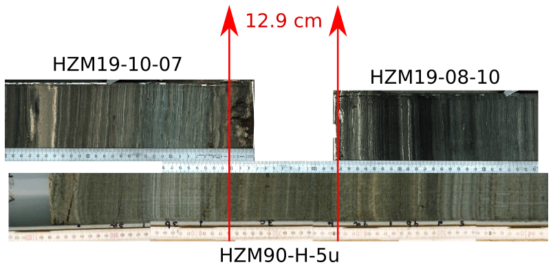
Figure A1Determination of the technical gap for HZM19 during the YD. This gap exists between sections HZM19-10-07 and HZM19-08-10 and is bridged by section HZM90-H5u from an earlier coring campaign.
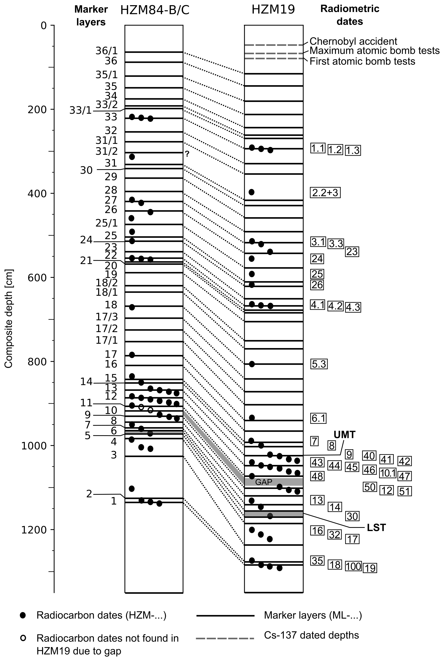
Figure A2Correlation of HZM84-B/C and HZM19. Positions of marker layers (MLs, indicated to the left) are marked as solid lines and connected by dotted lines between both profiles. Positions of radiocarbon dates (numbers indicated in rectangular boxes to the right) are marked as solid circles. Dotted grey horizontal lines refer to Cs-137-dated depths. The positions of the Ulmener Maar Tephra (UMT), Laacher See Tephra (LST), and the technical gap are indicated.
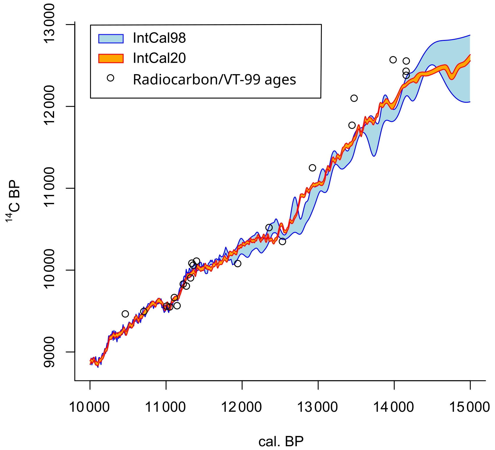
Figure A3Radiocarbon ages vs. Intcal98- and Intcal20-calibrated ages between 10 000 and 15 000 cal BP. Black circles show radiocarbon ages from Holzmaar vs. VT-99 age (reworked samples excluded). An underestimation of these ages occurs after 12 500 cal BP, where VT-99 seems to be too young.
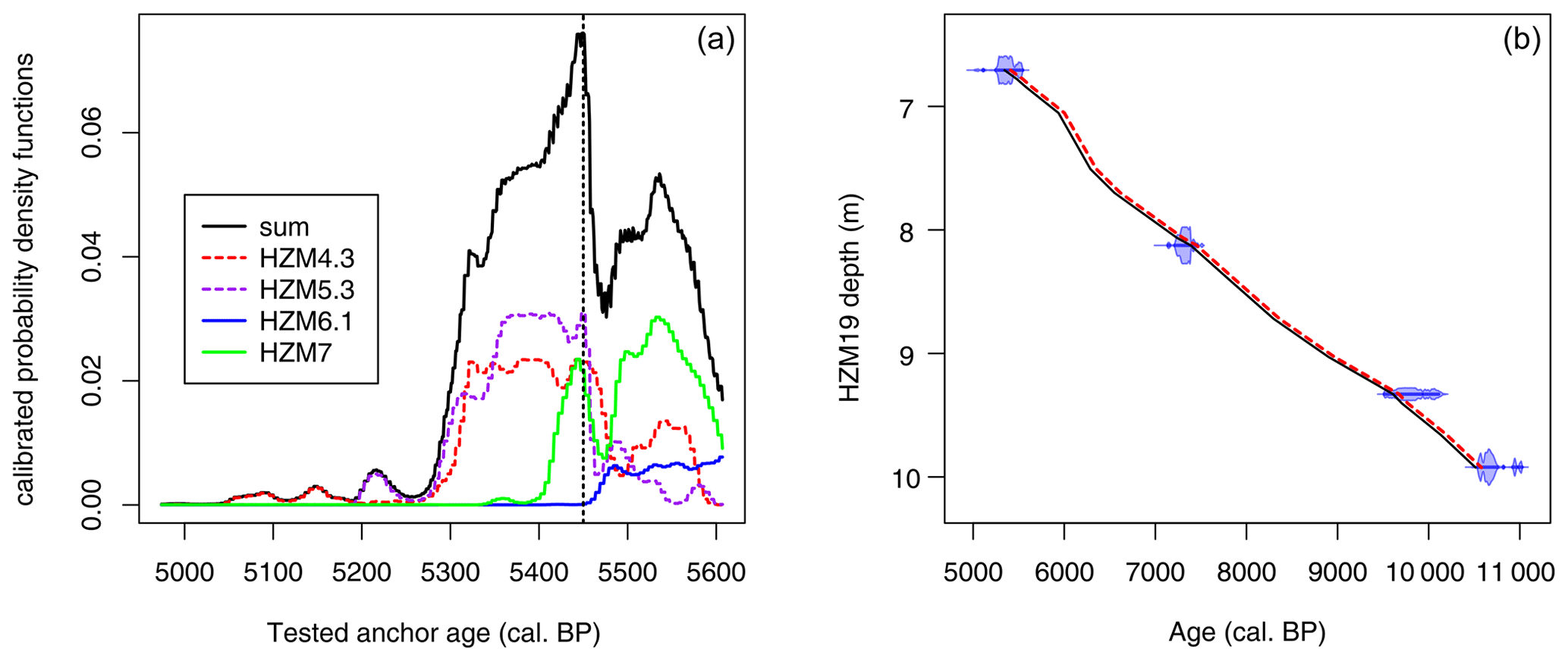
Figure A4Calculations for the floating VT-99 chronology of Model D, section 3. (a) Calculation of the anchoring age for the varve chronology based on matched and summed calibrated probability density function values of all radiocarbon samples within this section. The maximum summed probability occurs at an anchor age of 5450 cal BP. (b) Original VT-99 (black line) vs. floating VT-99 (+65 years, dotted red line) with calibrated radiocarbon samples vs. depth.
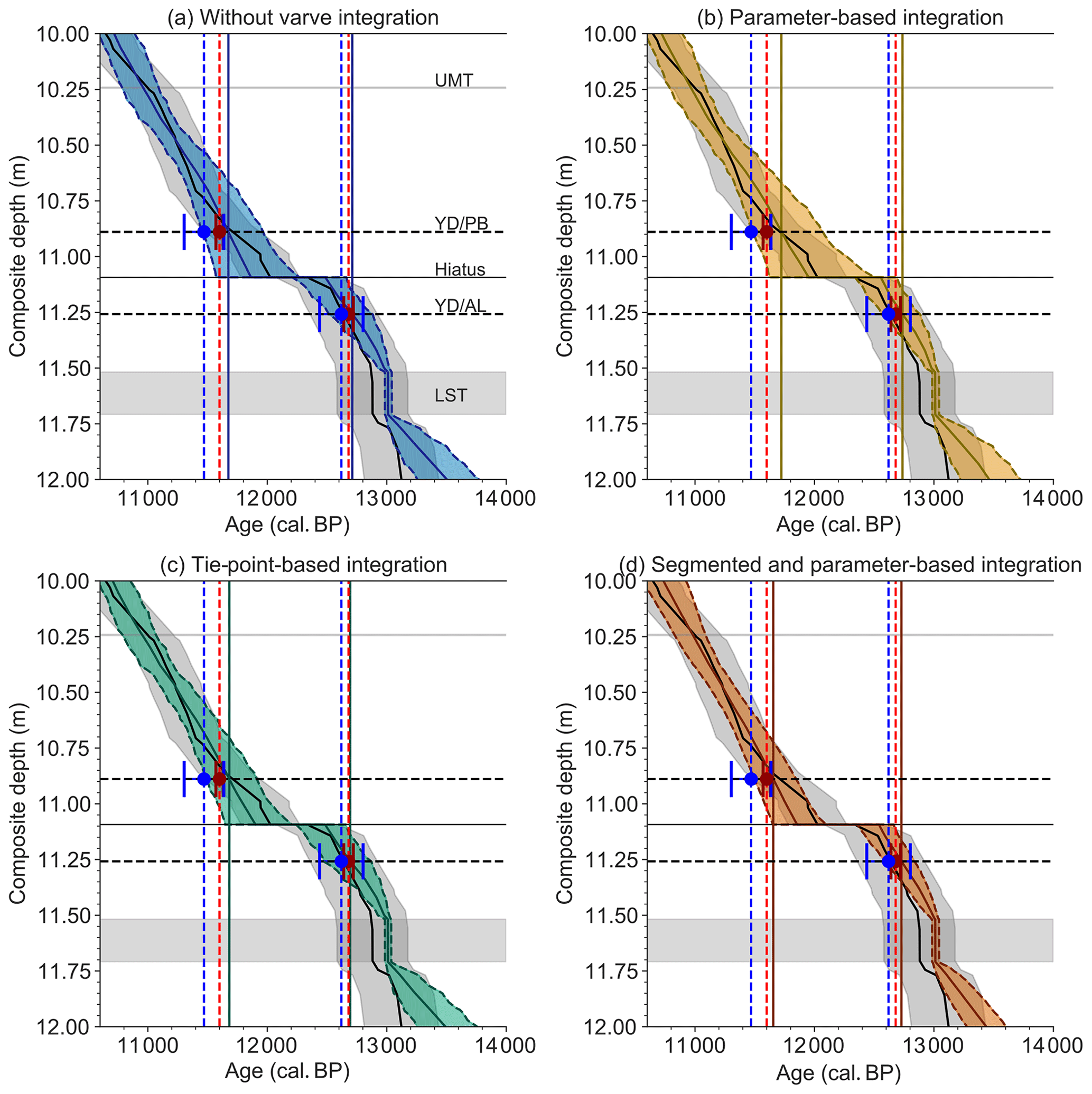
Figure A5Close-up plots for the Late Glacial to early Holocene transition for Models A (a), B (b), C (c), and D (d) with VT-99 mean age (solid black line) and error (shaded in grey) for comparison. Horizontal lines in all panels correspond to the labels in (a). Vertical lines refer to the Younger Dryas transitions for each model (solid lines), while dotted lines refer to mean ages derived by different sites (Lake Gosciaz in blue from Bonk et al., 2021; Meerfelder Maar in red from Brauer et al., 1999).
Table A1Core section and composite depths of lithozones H1 to H12 for HZM19.
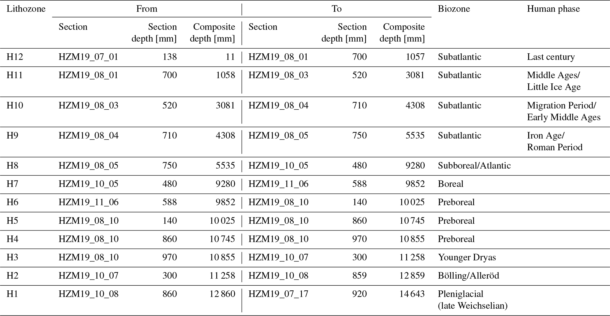
Table A2Error (1σ) estimations for different varve quality periods for the Holzmaar record (Zolitschka, 1998b), updated from VT-95 to VT-99.
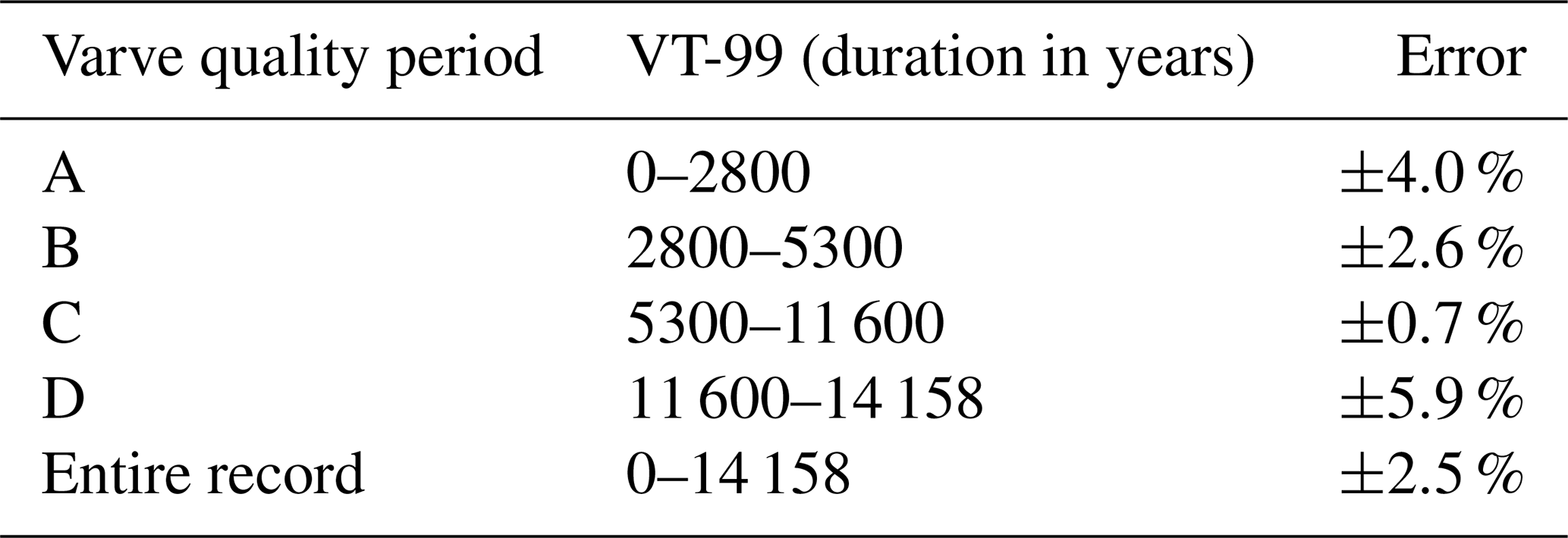
Table A3List of markers used for correlation of core sections in HZM19.

Table A4Core section depths of the composite profile HZM19 with resulting composite end depths for each core.

Table A5Marker layers (in italics) and radiocarbon dates (Hajdas et al., 2000, 1995, plus one unpublished radiocarbon date) vs. composite depth of HZM19. The calibrated median 14C age is calculated using OxCal with the IntCal20 calibration curve. Inconsistent calibrated ages are shown in brackets.
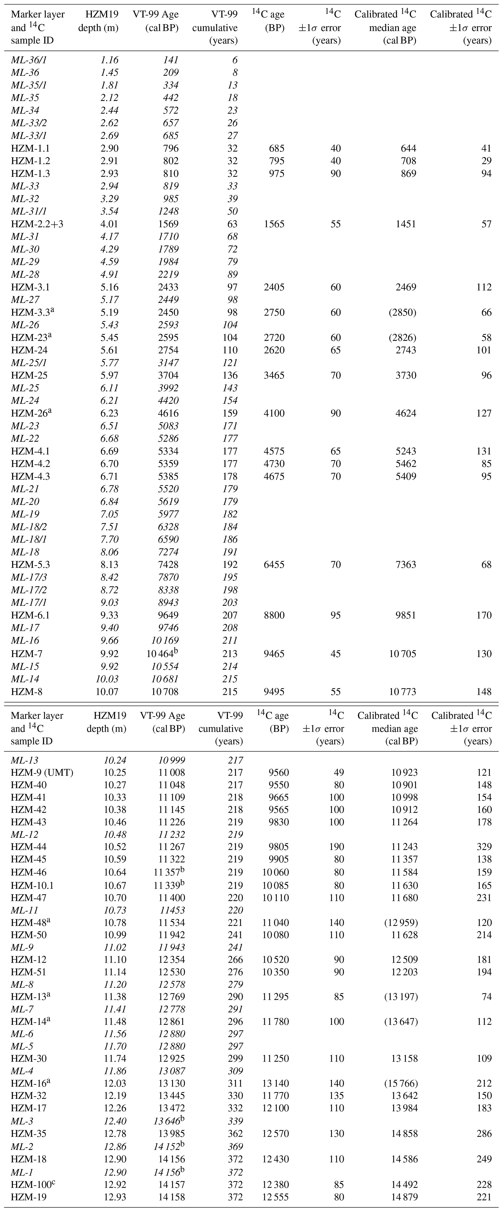
a Dates described to contain reworked organic material or being fractionated during graphitization (see Hajdas et al., 1995). b VT-99 dates excluded from modelling due to inconsistencies in documentation. c Unpublished radiocarbon age (KIA-1460).
Table A6Age estimations for VT-99 and Models A–D with their 95 % confidence intervals in brackets for the Ulmener Maar Tephra (UMT), the Younger Dryas–Preboreal-transition (YD/PB), the YD duration, the Allerød–Younger Dryas-transition (AL/YD), the predicted YD hiatus with duration and position, the Laacher See Tephra (LST), the maximum model age at 12.93 m with its mean and maximum age ranges, the position of the maximum age range, and the maximum difference between VT-99 and each of the model ranges.
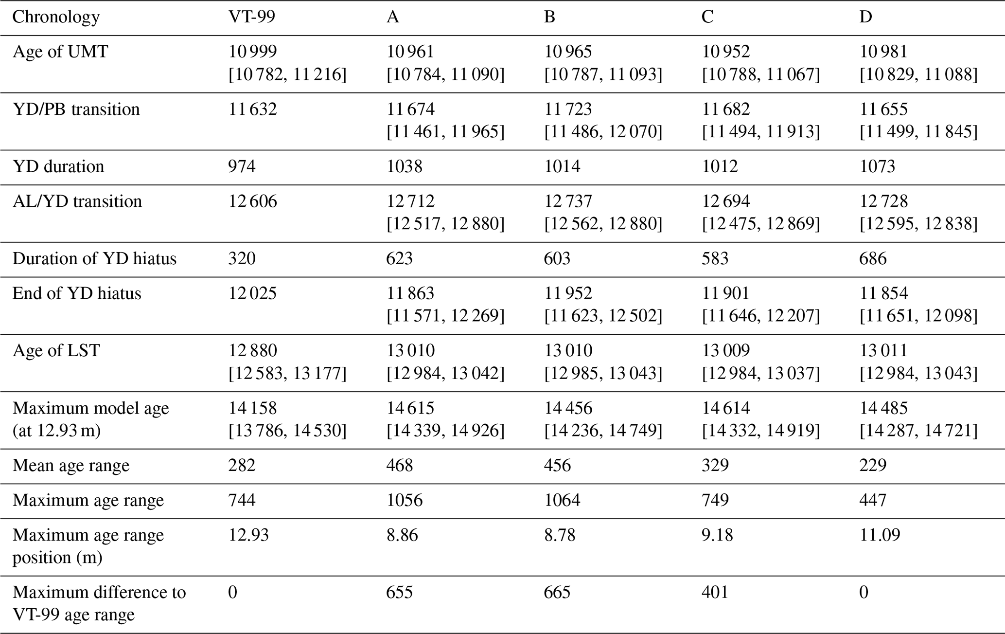
Table A7Additional dates for the HZM19 chronology with composite depths, ages (cal BP), and errors used for Bacon calculations. LST ages with error are from Reinig et al. (2021).
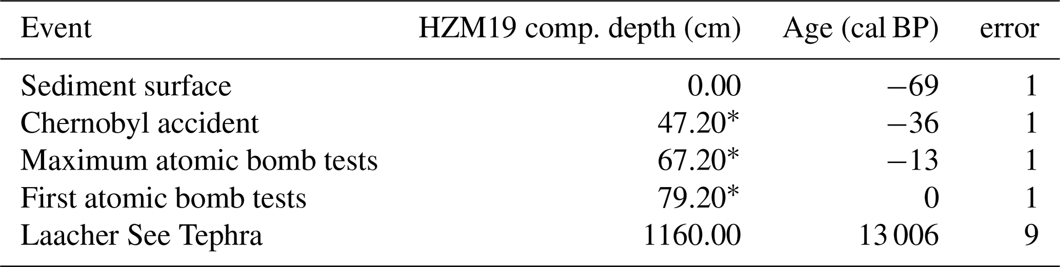
* 22 cm subtracted due to slump event documented by Pb-210 data.
The results of the different age–depth models carried out for the lacustrine sediment record from Holzmaar are accessible via the PANGAEA data-archiving and publication system at https://doi.org/10.1594/PANGAEA.949393 (Birlo et al., 2022).
SB and BZ conducted the fieldwork and conceptualized the study. SB described and sampled the sediment, modified and ran the Bayesian age–depth models, visualized the data, and drafted the first version of the manuscript. WT measured and interpreted lead and cesium data. All authors contributed to the writing and to revising of the manuscript.
The contact author has declared that none of the authors has any competing interests.
Publisher's note: Copernicus Publications remains neutral with regard to jurisdictional claims in published maps and institutional affiliations.
We would like to thank Christian Ohlendorf, Rafael Stiens, and An-Sheng Lee for participating in the coring campaign of 2019 and also for their subsequent help with core opening, sediment preparation, and scanning in the GEOPOLAR lab. Furthermore, we want to thank Maarten Blaauw, Arne Ramisch, and Alicja Bonk for helpful discussions.
This paper was edited by Irka Hajdas and reviewed by Natalia Piotrowska and one anonymous referee.
Anderson, R. Y. and Dean, W. E.: Lacustrine varve formation through time, Palaeogeogr. Palaeocl., 62, 215–235, https://doi.org/10.1016/0031-0182(88)90055-7, 1988.
Baier, J., Lücke, A., Negendank, J. F. W., Schleser, G.-H., and Zolitschka, B.: Diatom and geochemical evidence of mid- to late Holocene climatic changes at Lake Holzmaar, West-Eifel (Germany), Quaternary Int., 113, 81–96, https://doi.org/10.1016/S1040-6182(03)00081-8, 2004.
Battarbee, R. W., Howells, G. D., Skeffington, R. A., Bradshaw, A. D., Battarbee, R. W., Mason, B. J., Renberg, I., and Talling, J. F.: The causes of lake acidification, with special reference to the role of acid deposition, Philos. T. R. Soc. B, 327, 339–347, https://doi.org/10.1098/rstb.1990.0071, 1990.
Berglund, B. E. (Ed.): Handbook of Holocene Palaeoecology and Palaeohydrology, John Wiley & Sons Ltd., Chichester, 869 pp., 1986.
Birlo, S., Tylmann, W., and Zolitschka, B.: Bayesian age-depth modelling applied to varve counting and radiometric dating to develop a high-resolution chronology for a new composite sediment profile from Holzmaar (Germany), PANGAEA [data set], https://doi.org/10.1594/PANGAEA.949393, 2022.
Blaauw, M.: Methods and code for “classical” age-modelling of radiocarbon sequences, Quat. Geochronol., 5, 512–518, https://doi.org/10.1016/j.quageo.2010.01.002, 2010.
Blaauw, M. and Christen, J. A.: Flexible paleoclimate age-depth models using an autoregressive gamma process, Bayesian Anal., 6, 457–474, https://doi.org/10.1214/11-BA618, 2011.
Blaauw, M., Christen, J. A., Bennett, K. D., and Reimer, P. J.: Double the dates and go for Bayes – Impacts of model choice, dating density and quality on chronologies, Quaternary Sci. Rev., 188, 58–66, https://doi.org/10.1016/j.quascirev.2018.03.032, 2018.
Blaauw, M., Christen, J. A., Lopez, M. A. A., Vazquez, J. E., V, O. M. G., Belding, T., Theiler, J., Gough, B., and Karney, C.: rbacon: Age-Depth Modelling using Bayesian Statistics, CRAN [code], https://CRAN.R-project.org/package=rbacon (last access: 23 February 2022), 2021.
Bonk, A., Müller, D., Ramisch, A., Kramkowski, M. A., Noryœkiewicz, A. M., Sekudewicz, I., Ga̧siorowski, M., Luberda-Durnaś, K., Słowiński, M., Schwab, M., Tjallingii, R., Brauer, A., and Błaszkiewicz, M.: Varve microfacies and chronology from a new sediment record of Lake Gościa̧ż (Poland), Quaternary Sci. Rev., 251, 106715, https://doi.org/10.1016/j.quascirev.2020.106715, 2021.
Brauer, A.: Weichselzeitliche Seesedimente des Holzmaars – Warvenchronologie des Hochglazials und Nachweis von Klimaschwankungen, PhD thesis, Universität Trier, Documenta naturae, 85, 1–210, 1994.
Brauer, A., Hajdas, I., Negendank, J. F. W., Rein, B., Vos, H., and Zolitschka, B.: Warvenchronologie – eine Methode zur absoluten Datierung und Rekonstruktion kurzer und mittlerer solarer Periodizitäten, Geowissenschaften, 12, 325–332, 1994.
Brauer, A., Endres, C., Günter, C., Litt, T., Stebich, M., and Negendank, J. F. W.: High resolution sediment and vegetation responses to Younger Dryas climate change in varved lake sediments from Meerfelder Maar, Germany, Quaternary Sci. Rev., 18, 321–329, https://doi.org/10.1016/S0277-3791(98)00084-5, 1999.
Bronk Ramsey, C.: Deposition models for chronological records, Quaternary Sci. Rev., 27, 42–60, https://doi.org/10.1016/j.quascirev.2007.01.019, 2008.
Brooks, S. P. and Gelman, A.: General Methods for Monitoring Convergence of Iterative Simulations, J. Comput. Graph. Stat., 7, 434–455, https://doi.org/10.1080/10618600.1998.10474787, 1998.
Büchel, G.: Maars of the Westeifel, Germany, in: Paleolimnology of European Maar Lakes, edited by: Negendank, J. F. W. and Zolitschka, B., Springer, Berlin, Heidelberg, 1–13, https://doi.org/10.1007/BFb0117585, 1993.
Cohen, A. S.: Paleolimnology. The history and evolution of lake systems, Oxford University Press, Oxford, 500 pp., ISBN 0-19-513353-6, 2003.
Davies, S. M.: Cryptotephras: the revolution in correlation and precision dating, J. Quaternary Sci., 30, 114–130, https://doi.org/10.1002/jqs.2766, 2015.
De Geer, G.: A geochronology of the last 12,000 years, Proceedings of the International Geological Congress, Stockholm (1910), 1, 241–253, 1912.
Dean, W. E., Bradbury, J. P., Anderson, R. Y., and Barnosky, C. W.: The Variability of Holocene Climate Change: Evidence from Varved Lake Sediments, Science, 226, 1191–1194, https://doi.org/10.1126/science.226.4679.1191, 1984.
Fortin, D., Praet, N., McKay, N. P., Kaufman, D. S., Jensen, B. J. L., Haeussler, P. J., Buchanan, C., and De Batist, M.: New approach to assessing age uncertainties – The 2300-year varve chronology from Eklutna Lake, Alaska (USA), Quaternary Sci. Rev., 203, 90–101, https://doi.org/10.1016/j.quascirev.2018.10.018, 2019.
García, M. L., Birlo, S., and Zolitschka, B.: Paleoenvironmental changes of the last 16,000 years based on diatom and geochemical stratigraphies from the varved sediment of Holzmaar (West-Eifel Volcanic Field, Germany), Quaternary Sci. Rev., 293, 107691, https://doi.org/10.1016/j.quascirev.2022.107691, 2022.
Goslar, T., Kuc, T., Ralska-Jasiewiczowa, M., Rózánski, K., Arnold, M., Bard, E., van Geel, B., Pazdur, M., Szeroczyńska, K., Wicik, B., Wiȩckowski, K., and Walanus, A.: High-resolution lacustrine record of the late glacial/holocene transition in central Europe, Quaternary Sci. Rev., 12, 287–294, https://doi.org/10.1016/0277-3791(93)90037-M, 1993.
Hajdas, I., Zolitschka, B., Ivy-Ochs, S. D., Beer, J., Bonani, G., Leroy, S. A. G., Negendank, J. W., Ramrath, M., and Suter, M.: AMS radiocarbon dating of annually laminated sediments from lake Holzmaar, Germany, Quaternary Sci. Rev., 14, 137–143, https://doi.org/10.1016/0277-3791(94)00123-S, 1995.
Hajdas, I., Bonani, G., and Zolitschka, B.: Radiocarbon Dating of Varve Chronologies: Soppensee and Holzmaar Lakes after Ten Years, Radiocarbon, 42, 349–353, https://doi.org/10.1017/S0033822200030290, 2000.
Hajdas-Skowronek, I.: Extension of the radiocarbon calibration curve by AMS dating of laminated sediments of Lake Soppensee and Lake Holzmaar, PhD thesis, ETH Zurich, https://doi.org/10.3929/ETHZ-A-000916163, 1993.
Haslett, J. and Parnell, A.: A simple monotone process with application to radiocarbon-dated depth chronologies, J. R. Stat. Soc. C-Appl., 57, 399–418, https://doi.org/10.1111/j.1467-9876.2008.00623.x, 2008.
Jenny, J.-P., Koirala, S., Gregory-Eaves, I., Francus, P., Niemann, C., Ahrens, B., Brovkin, V., Baud, A., Ojala, A. E. K., Normandeau, A., Zolitschka, B., and Carvalhais, N.: Human and climate global-scale imprint on sediment transfer during the Holocene, P. Natl. Acad. Sci. USA, 116, 22972–22976, https://doi.org/10.1073/pnas.1908179116, 2019.
Kelts, K., Briegel, U., Ghilardi, K., and Hsu, K.: The limnogeology-ETH coring system, Schweiz. Z. Hydrol., 48, 104–115, https://doi.org/10.1007/BF02544119, 1986.
Kienel, U., Schwab, M. J., and Schettler, G.: Distinguishing climatic from direct anthropogenic influences during the past 400 years in varved sediments from Lake Holzmaar (Eifel, Germany), J. Paleolimnol., 33, 327–347, https://doi.org/10.1007/s10933-004-6311-z, 2005.
Lacourse, T. and Gajewski, K.: Current practices in building and reporting age-depth models, Quaternary Res., 96, 28–38, https://doi.org/10.1017/qua.2020.47, 2020.
Lamoureux, S.: Varve Chronology Techniques, in: Tracking Environmental Change Using Lake Sediments: Basin Analysis, Coring, and Chronological Techniques, edited by: Last, W. M. and Smol, J. P., Springer Netherlands, Dordrecht, 247–260, https://doi.org/10.1007/0-306-47669-X_11, 2001.
Last, W. M. and Smol, J. P. (Eds.): Tracking Environmental Change Using Lake Sediments, Vol. 1, Basin Analysis, Coring, and Chronological Techniques, Springer Netherlands, Dordrecht, 548 pp., eBook ISBN 0-306-47669-X, Print ISBN 0-7923-6482-1 2001a.
Last, W. M. and Smol, J. P. (Eds.): Tracking Environmental Change Using Lake Sediments, Vol. 2, Physical and Geochemical Methods, Springer Netherlands, Dordrecht, 504 pp., eBook ISBN 0-306-47670-3, Print ISBN 1-4020-0628-4, 2001b.
Leroy, S. A. G., Zolitschka, B., Negendank, J. F. W., and Seret, G.: Palynological analyses in the laminated sediment of Lake Holzmaar (Eifel, Germany): duration of Lateglacial and Preboreal biozones, Boreas, 29, 52–71, https://doi.org/10.1111/j.1502-3885.2000.tb01200.x, 2000.
Litt, T., Schölzel, C., Kühl, N., and Brauer, A.: Vegetation and climate history in the Westeifel Volcanic Field (Germany) during the past 11 000 years based on annually laminated lacustrine maar sediments, Boreas, 38, 679–690, https://doi.org/10.1111/j.1502-3885.2009.00096.x, 2009.
Lorenz, V.: Explosive Volcanism of the West Eifel Volcanic Field/Germany, in: Developments in Petrology, Vol. 11, edited by: Kornprobst, J., Elsevier, 299–307, https://doi.org/10.1016/B978-0-444-42273-6.50026-2, 1984.
Lorenz, V., Lange, T., and Büchel, G.: Die Vulkane der Westeifel, Jahresberichte und Mitteilungen des Oberrheinischen Geologischen Vereins, 102, 379–411, https://doi.org/10.1127/jmogv/102/0022, 2020.
Lotter, A. F.: Absolute Dating of the Late-Glacial Period in Switzerland Using Annually Laminated Sediments, Quaternary Res., 35, 321–330, https://doi.org/10.1016/0033-5894(91)90048-A, 1991.
Lücke, A., Schleser, G. H., Zolitschka, B., and Negendank, J. F. W.: A Lateglacial and Holocene organic carbon isotope record of lacustrine palaeoproductivity and climatic change derived from varved lake sediments of Lake Holzmaar, Germany, Quaternary Sci. Rev., 22, 569–580, https://doi.org/10.1016/S0277-3791(02)00187-7, 2003.
Martin-Puertas, C., Walsh, A. A., Blockley, S. P. E., Harding, P., Biddulph, G. E., Palmer, A., Ramisch, A., and Brauer, A.: The first Holocene varve chronology for the UK: Based on the integration of varve counting, radiocarbon dating and tephrostratigraphy from Diss Mere (UK), Quat. Geochronol., 61, 101134, https://doi.org/10.1016/j.quageo.2020.101134, 2021.
Meyer, W.: Zur Entstehung der Maare in der Eifel, Z. Dtsch. Ges. Geowiss., 136, 141–155, https://doi.org/10.1127/zdgg/136/1985/141, 1985.
Meyer, W.: Geologie der Eifel, 4th Edn., Schweizerbart Science Publishers, Stuttgart, Germany, ISBN 978-3-510-65279-2, 2013.
Meyer, W. and Stets, J.: Pleistocene to Recent tectonics in the Rhenish Massif (Germany), Neth. J. Geosci., 81, 217–221, https://doi.org/10.1017/S0016774600022460, 2002.
Muggeo, V. M. R.: segmented: Regression Models with Break-Points/Change-Points Estimation, CRAN [code], https://CRAN.R-project.org/package=segmented, last access: 23 February 2022.
Nesje, A., Søgnen, K., Elgersma, A., and Dahl, S. O.: A Piston Corer for Lake Sediments, Norsk. Geogr. Tidsskr., 41, 123–125, https://doi.org/10.1080/00291958708621986, 1987.
Olsson, I. U.: Radometric dating, in: Handbook of Holocene Palaeoecology and Palaeohydrology, edited by: Berglund, B. E., John Wiley & Sons, Chichester, 273–312, ISBN 0 471 90691 3, 1986.
O'Sullivan, P. E.: Annually-laminated lake sediments and the study of Quaternary environmental changes – a review, Quaternary Sci. Rev., 1, 245–313, https://doi.org/10.1016/0277-3791(83)90008-2, 1983.
Pearson, G. W., Pilcher, J. R., Baillie, M. G. L., and Hillam, J.: Absolute radiocarbon dating using a low altitude European tree-ring calibration, Nature, 270, 25–28, https://doi.org/10.1038/270025a0, 1977.
Prasad, S. and Baier, J.: Tracking the impact of mid- to late Holocene climate change and anthropogenic activities on Lake Holzmaar using an updated Holocene chronology, Global Planet. Change, 122, 251–264, https://doi.org/10.1016/j.gloplacha.2014.08.020, 2014.
R Core Team: R: A Language and Environment for Statistical Computing, R Foundation for Statistical Computing, Vienna, Austria, https://www.r-project.org/, last access: 25 September 2021.
Reimer, P. J., Austin, W. E. N., Bard, E., Bayliss, A., Blackwell, P. G., Bronk Ramsey, C., Butzin, M., Cheng, H., Edwards, R. L., Friedrich, M., Grootes, P. M., Guilderson, T. P., Hajdas, I., Heaton, T. J., Hogg, A. G., Hughen, K. A., Kromer, B., Manning, S. W., Muscheler, R., Palmer, J. G., Pearson, C., van der Plicht, J., Reimer, R. W., Richards, D. A., Scott, E. M., Southon, J. R., Turney, C. S. M., Wacker, L., Adolphi, F., Büntgen, U., Capano, M., Fahrni, S. M., Fogtmann-Schulz, A., Friedrich, R., Köhler, P., Kudsk, S., Miyake, F., Olsen, J., Reinig, F., Sakamoto, M., Sookdeo, A., and Talamo, S.: The INTCAL20 Northern Hemisphere Radiocarbon Age Calibration Curve (0–55 cal kBP), Radiocarbon, 62, 725–757, https://doi.org/10.1017/RDC.2020.41, 2020.
Reinig, F., Wacker, L., Jöris, O., Oppenheimer, C., Guidobaldi, G., Nievergelt, D., Adolphi, F., Cherubini, P., Engels, S., Esper, J., Land, A., Lane, C., Pfanz, H., Remmele, S., Sigl, M., Sookdeo, A., and Büntgen, U.: Precise date for the Laacher See eruption synchronizes the Younger Dryas, Nature, 595, 66–69, https://doi.org/10.1038/s41586-021-03608-x, 2021.
Renberg, I. and Hansson, H.: A pump freeze corer for recent sediments, Limnol. Oceanogr., 38, 1317–1321, https://doi.org/10.4319/lo.1993.38.6.1317, 1993.
Renberg, I., Persson, M. W., and Emteryd, O.: Pre-industrial atmospheric lead contamination detected in Swedish lake sediments, Nature, 368, 323–326, https://doi.org/10.1038/368323a0, 1994.
Saarnisto, M.: Long varve series in Finland, Boreas, 14, 133–137, https://doi.org/10.1111/j.1502-3885.1985.tb00905.x, 1985.
Saarnisto, M.: Annually laminated lake sediments, in: Handbook of Holocene palaeoecology and palaeohydrology, edited by: Berglund, B. E., John Wiley and Sons Ltd, Chichester, 343–370, ISBN 0 471 90691 3, 1986.
Scharf, B.: Limnologische Beschreibung, Nutzung und Unterhaltung von Eifelmaaren, Ministerium für Umwelt und Gesundheit Rheinland-Pfalz, Mainz, ISBN 880253746, 1987.
Scharf, B. W. and Oehms, M.: Physical and chemical characteristics, in: Limnology of Eifel maar lakes. Ergebnisse der Limnologie, Vol. 38, edited by: Scharf, B. W. and Björk, S., E. Schweizerbart, Stuttgart, 63–83, ISBN 978-3-510-47039-6, 1992.
Schmincke, H.-U.: The Quaternary Volcanic Fields of the East and West Eifel (Germany), in: Mantle Plumes: A Multidisciplinary Approach, edited by: Ritter, J. R. R. and Christensen, U. R., Springer, Berlin, Heidelberg, 241–322, https://doi.org/10.1007/978-3-540-68046-8_8, 2007.
Schmincke, H.-U.: Vulkane der Eifel, 2nd Edn., Springer, Berlin, Heidelberg, https://doi.org/10.1007/978-3-8274-2985-8, 2014.
Schnurrenberger, D., Russell, J., and Kelts, K.: Classification of lacustrine sediments based on sedimentary components, J. Paleolimnol., 29, 141–154, https://doi.org/10.1023/A:1023270324800, 2003.
Shanahan, T. M., Beck, J. W., Overpeck, J. T., McKay, N. P., Pigati, J. S., Peck, J. A., Scholz, C. A., Heil, C. W., and King, J.: Late Quaternary sedimentological and climate changes at Lake Bosumtwi Ghana: New constraints from laminae analysis and radiocarbon age modeling, Palaeogeogr. Palaeocl., 361–362, 49–60, https://doi.org/10.1016/j.palaeo.2012.08.001, 2012.
Sirocko, F., Dietrich, S., Veres, D., Grootes, P. M., Schaber-Mohr, K., Seelos, K., Nadeau, M.-J., Kromer, B., Rothacker, L., Röhner, M., Krbetschek, M., Appleby, P., Hambach, U., Rolf, C., Sudo, M., and Grim, S.: Multi-proxy dating of Holocene maar lakes and Pleistocene dry maar sediments in the Eifel, Germany, Quaternary Sci. Rev., 62, 56–76, https://doi.org/10.1016/j.quascirev.2012.09.011, 2013.
Stuiver, M., Reimer, P. J., Bard, E., Beck, J. W., Burr, G. S., Hughen, K. A., Kromer, B., McCormac, G., Van Der Plicht, J., and Spurk, M.: INTCAL98 Radiocarbon Age Calibration, 24,000–0 cal BP, Radiocarbon, 40, 1041–1083, https://doi.org/10.1017/S0033822200019123, 1998.
Telford, R., Heegaard, E., and Birks, H.: All age–depth models are wrong: but how badly?, Quaternary Sci. Rev., 23, 1–5, https://doi.org/10.1016/j.quascirev.2003.11.003, 2004.
Trachsel, M. and Telford, R. J.: All age–depth models are wrong, but are getting better, Holocene, 27, 860–869, https://doi.org/10.1177/0959683616675939, 2017.
Turkey, C. S. M. and Lowe, J. J.: Tephrochronology, in: Tracking Environmental Change Using Lake Sediments: Basin Analysis, Coring, and Chronological Techniques, edited by: Last, W. M. and Smol, J. P., Springer Netherlands, Dordrecht, 451–471, https://doi.org/10.1007/0-306-47669-X_16, 2001.
Vandergoes, M. J., Howarth, J. D., Dunbar, G. B., Turnbull, J. C., Roop, H. A., Levy, R. H., Li, X., Prior, C., Norris, M., Keller, L. D., Baisden, W. T., Ditchburn, R., Fitzsimons, S. J., and Bronk Ramsey, C.: Integrating chronological uncertainties for annually laminated lake sediments using layer counting, independent chronologies and Bayesian age modelling (Lake Ohau, South Island, New Zealand), Quaternary Sci. Rev., 188, 104–120, https://doi.org/10.1016/j.quascirev.2018.03.015, 2018.
Wright, H. E., Mann, D. H., and Glaser, P. H.: Piston Corers for Peat and Lake Sediments, Ecology, 65, 657–659, https://doi.org/10.2307/1941430, 1984.
Zolitschka, B.: Spätquartäre Sedimentationsgeschichte des Meerfelder Maares (Westeifel).–Mikrostratigraphie jahreszeitlich geschichteter Seesedimente, E&G Quaternary Sci. J., 38, 87–93, https://doi.org/10.3285/eg.38.1.08, 1988.
Zolitschka, B.: Jahreszeitlich geschichtete Seesedimente aus dem Holzmaar und dem Meerfelder Maar, Z. Dtsch. Ges. Geowiss., 140, 25–33, https://doi.org/10.1127/zdgg/140/1989/25, 1989.
Zolitschka, B.: Jahreszeitlich geschichtete Seesedimente ausgewählter Eifelmaare – paläolimnologische Untersuchung als Beitrag zur spät- und postglazialen Klima- und Besiedlungsgeschichte, PhD thesis, Universität Trier, Documenta naturae, 60, 226 pp., 1990.
Zolitschka, B.: Absolute dating of late Quaternary Lacustrine sediments by high resolution varve chronology, Hydrobiologia, 214, 59–61, https://doi.org/10.1007/BF00050932, 1991.
Zolitschka, B.: Climatic change evidence and lacustrine varves from maar lakes, Germany, Clim. Dynam., 6, 229–232, https://doi.org/10.1007/BF00193535, 1992.
Zolitschka, B.: A 14,000 year sediment yield record from western Germany based on annually laminated lake sediments, Geomorphology, 22, 1–17, https://doi.org/10.1016/S0169-555X(97)00051-2, 1998a.
Zolitschka, B.: Paläoklimatische Bedeutung laminierter Sedimente: Holzmaar (Eifel, Deutschland), Lake C2 (Northwest-Territorien, Kanada) und Lago Grande di Monticchio (Basilicata, Italien), Habil. thesis, Universität Potsdam, Relief Boden Paläoklima, 13, 176 pp., 1998b.
Zolitschka, B., Haverkamp, B., and Negendank, J. F. W.: Younger Dryas Oscillation – Varve Dated Microstratigraphic, Palynological and Palaeomagnetic Records from Lake Holzmaar, Germany, in: The Last Deglaciation: Absolute and Radiocarbon Chronologies, edited by: Bard, E. and Broecker, W. S., Springer Berlin Heidelberg, Berlin, Heidelberg, 81–101, https://doi.org/10.1007/978-3-642-76059-4_6, 1992.
Zolitschka, B., Brauer, A., Negendank, J. F. W., Stockhausen, H., and Lang, A.: Annually dated late Weichselian continental paleoclimate record from the Eifel, Germany, Geology, 28, 783–786, https://doi.org/10.1130/0091-7613(2000)28<783:ADLWCP>2.0.CO;2, 2000.
Zolitschka, B., Francus, P., Ojala, A. E. K., and Schimmelmann, A.: Varves in lake sediments – a review, Quaternary Sci. Rev., 117, 1–41, https://doi.org/10.1016/j.quascirev.2015.03.019, 2015.
- Abstract
- Introduction
- Regional settings and the Holzmaar sediment record
- Materials and methods
- Results and interpretation
- Evaluation of different varve integration techniques
- Conclusion
- Appendix A
- Data availability
- Author contributions
- Competing interests
- Disclaimer
- Acknowledgements
- Review statement
- References