the Creative Commons Attribution 4.0 License.
the Creative Commons Attribution 4.0 License.
 | 07 Feb 2023
Calculation of uncertainty in the (U–Th) ∕ He system
Peter E. Martin
James R. Metcalf
Rebecca M. Flowers
Although rigorous uncertainty reporting on (U–Th) He dates is key for interpreting the expected distributions of dates within individual samples and for comparing dates generated by different labs, the methods and formulae for calculating single-grain uncertainty have never been fully described and published. Here we publish two procedures to derive (U–Th) He single-grain date uncertainty (linear and Monte Carlo uncertainty propagation) based on input 4He, radionuclide, and isotope-specific FT (alpha-ejection correction) values and uncertainties. We also describe a newly released software package, HeCalc, that performs date calculation and uncertainty propagation for (U–Th) He data. Propagating uncertainties in 4He and radionuclides using a compilation of real (U–Th) He data (N=1978 apatites and 1753 zircons) reveals that the uncertainty budget in this dataset is dominated by uncertainty stemming from the radionuclides, yielding median relative uncertainty values of 2.9 % for apatite dates and 1.7 % for zircon dates (1 s equivalent). When uncertainties in FT of 2 % or 5 % are assumed and additionally propagated, the median relative uncertainty values increase to 3.5 % and 5.8 % for apatite dates and 2.6 % and 5.2 % for zircon dates. The potentially strong influence of FT on the uncertainty budget underscores the importance of ongoing efforts to better quantify and routinely propagate FT uncertainty into (U–Th) He dates. Skew is generally positive and can be significant, with ∼ 17 % of apatite dates and ∼ 6 % of zircon dates in the data compilation characterized by skewness of 0.25 or greater assuming 2 % uncertainty in FT. This outcome indicates the value of applying Monte Carlo uncertainty propagation to identify samples with substantially asymmetric uncertainties that should be considered during data interpretation. The formulae published here and the associated HeCalc software can aid in more consistent and rigorous (U–Th) He uncertainty reporting, which is also a key first step in quantifying whether multiple aliquots from a sample are over-dispersed, with dates that differ beyond what is expected from analytical and FT uncertainties.
- Article
(3551 KB) - Full-text XML
- BibTeX
- EndNote


The (U–Th) He method for geochronology and thermochronology was initially developed as a reliable technique approximately 3 decades ago (Farley et al., 1996; Wernicke and Lippolt, 1994; Wolf et al., 1996; Zeitler et al., 1987). Since that time, numerous advances such as the ability to measure the (U–Th) He date of individual grains (e.g., House et al., 2000), improvements in kinetic models to account for the effects of radiation damage accumulation and annealing on He diffusion kinetics (e.g., Flowers et al., 2009; Gautheron et al., 2009; Guenthner et al., 2013), and the development of thermal history modeling tools that improve interpretation of these data (Gallagher, 2012; Ketcham, 2005) have led to the widespread application of this technique and large amounts of data generation. However, with this progress has come recognition of the need to more rigorously and consistently report uncertainties in individual (U–Th) He dates (Flowers et al., 2022; Ketcham et al., 2022). For example, the intra-sample variability of (U–Th) He dates often exceeds that predicted by analytical uncertainty due to differences in He diffusion kinetics among grains and scatter from other factors (e.g., Brown et al., 2013; Fitzgerald et al., 2006; Flowers et al., 2022b). Better accounting for the uncertainties of individual analyses is a key step in determining whether multiple individual analyses from a sample are actually “over-dispersed” and would help develop a more complete understanding of the causes of data dispersion by allowing the scatter attributable to analytical uncertainty to be subtracted from the overall dispersion pattern. In addition, more rigorous uncertainty reporting would improve confidence in large-N datasets, facilitate inter-laboratory data comparisons, and ultimately increase the precision and accuracy of thermal history reconstructions.
One current challenge to comprehensive uncertainty propagation is that, although individual laboratories have derived the methods for propagating uncertainty components into single-grain (U–Th) He dates, these methods and the resulting formal analytical uncertainty in (U–Th) He dates have never been described or thoroughly assessed in the literature. It also is unclear if different labs propagate uncertainties in the same manner. Uncertainty propagation in the (U–Th) He system is complicated by the fact that the age equation has no analytical solution, precluding the direct application of typical uncertainty propagation formulae that combine individual uncertainty components in quadrature through a given function. This problem may be circumvented by approximations of the He age equation that solve directly for time (e.g., Meesters and Dunai, 2005) or by the use of the general “error propagation equation” using the first derivatives of the uncertainty components with respect to time (Bevington and Robinson, 2003). However, linear uncertainty propagation methods rely on an assumption that the derivative of the first term of the Taylor series is a linear function at the scale of the uncertainties being combined (Bevington and Robinson, 2003; McLean et al., 2011). As this assumption is often violated in the (U–Th) He system, uncertainties have the potential to be skewed (i.e., asymmetric), and uncertainties propagated using standard linear uncertainty propagation may be inaccurate.
Comprehensive uncertainty accounting in individual (U–Th) He dates involves propagating not only the analytical uncertainties associated with measurements of parent and daughter amounts, but also propagating uncertainties associated with alpha-ejection corrections (FT corrections, which account for He ejected from the crystal via alpha decay). The analytical uncertainty on parent and daughter amounts is generally well-characterized, and the geometric uncertainty in FT values is increasingly well-constrained (e.g., Cooperdock et al., 2019; Glotzbach et al., 2019; Zeigler et al., 2022). As FT uncertainties are better quantified, propagating both analytical and FT uncertainties into the reported uncertainty of (U–Th) He dates is desirable (e.g., Flowers et al., 2022a).
Here we explain how analytical and FT uncertainties in (U–Th) He dates may be combined to derive a single-grain (U–Th) He date uncertainty. To address the shortcomings of linear uncertainty propagation, we primarily adopt a Monte Carlo approach to quantitatively constrain (U–Th) He uncertainty. This procedure is both accurate and mathematically simple, and it enables evaluation of asymmetric uncertainties (which linear uncertainty propagation does not provide). For completeness and to ease retrospective data comparisons, we also include a method to compute date uncertainty that uses more traditional linear uncertainty propagation. In addition, this paper presents a new program written in Python 3.8 termed HeCalc (Helium date and uncertainty Calculator; Martin, 2022) that is capable of both Monte Carlo and linear methods of uncertainty propagation. We conclude by using HeCalc to reduce a compilation of real data to determine the typical contributions of each uncertainty component to date uncertainty in actual practice.
The currently quantifiable uncertainties in single-grain (U–Th) He dates include analytical uncertainties associated with parent and daughter isotopic measurements and geometric uncertainties associated with FT corrections. These are discussed in detail in Flowers et al. (2022a) and summarized more briefly here. We use the word “uncertainty” as a probabilistic statement of the distribution of repeated measurements (e.g., for a 238U measurement of 10 ± 1 µg g−1 at 1σ, 68.27 % of repeated measurements will fall between 9 and 11 µg g−1), while “error” refers to the deviation of a measured value from the true value. The uncertainty in decay constants is negligible relative to other sources of uncertainty and causes systematic error across all (U–Th) He measurements; it is therefore not incorporated in our uncertainty calculation methods.
In the (U–Th) He technique, the parent nuclides (uranium, thorium, and samarium; 238U, 235U, 232Th, 147Sm) are typically measured using inductively coupled plasma mass spectrometry (ICP-MS), while the daughter product (helium; 4He) is usually measured on a quadrupole or magnetic sector noble gas mass spectrometer. Most commonly, quantification of 4He and its parent nuclides is performed via isotope dilution to permit conversion from isotopic ratio measurements to molar amounts. Given the measurements of parent and daughter products, a (U–Th) He date may be calculated using the equation for 4He ingrowth.
Here, each nuclide is given as an amount, t is time, and λ is the decay constant for each parent nuclide given in the subscript.
Because of the kinetic energy associated with alpha decay, individual alpha particles (i.e., 4He nuclei) travel between 4 and 34 µm in solid matter before coming to rest, depending on the mineral density and parent or intermediate daughter nuclide (Farley et al., 1996; Ketcham et al., 2011). This redistribution of the daughter product can cause He ejection from a crystal. By assuming a homogenous parent nuclide distribution, measuring the physical dimensions of a single grain, and applying a geometric model to those physical dimensions, the proportion of alpha particles retained in a grain (the fraction trapped; FT) can be calculated for each nuclide's mean stopping distance (Ketcham et al., 2011). Determination of grain dimensions to calculate FT is usually accomplished via size measurement of individual grains using photomicrographs with a calibrated digital camera (Cooperdock et al., 2019; Glotzbach et al., 2019). Using the FT parameter, the effects of alpha ejection on a date can be corrected using a modified version of the 4He ingrowth equation with the isotope-specific FT values (, , , FT) included (Ketcham et al., 2011).
We refer to dates calculated with this correction applied as “alpha-ejection-corrected” or simply “corrected” dates, while dates calculated with no correction applied using Eq. (1) are referred to as “uncorrected” or “raw” dates.
For this work, it is assumed that the amount and uncertainty of each nuclide have been constrained. The natural U isotopic ratio (137.818 ± 0.023 1 s; Hiess et al., 2012) is usually used to calculate 235U in a sample based on the 238U amount measured. In these cases, the uncertainty in 235U is perfectly correlated with 238U; treatment of these uncertainties as though they were independent could lead to inaccurate uncertainty calculations. Whether or not the uncertainty in the other radionuclides is correlated depends on the details of isotope spiking procedures and must be evaluated on an individual lab basis.
Uncertainty and systematic error in FT values likely stem from a combination of inaccurate grain measurements, assumptions regarding the specific geometry of a given grain (i.e., deviations from the “idealized” shapes in Ketcham et al., 2011), and undetected parent nuclide zonation (e.g., Farley et al., 1996). When the magnitudes of these effects are constrained then the corresponding uncertainties can be propagated into the FT value uncertainty and FT values can be corrected for systematic error. Several approaches have been developed to approximate the 3D shape of individual grains to assess uncertainty associated with grain geometry estimates, generally finding that the geometric uncertainty in FT ranges between 2 %–8 % and 1 s (Cooperdock et al., 2019; Evans et al., 2008; Glotzbach et al., 2019; Herman et al., 2007; Zeigler et al., 2022). The magnitude of systematic error depends on grain shape and the details of the method used for FT value determination (e.g., Cooperdock et al., 2019; Glotzbach et al., 2019; Zeigler et al., 2022). Measurement of parent nuclide zonation is not currently done in typical workflows, so this source of uncertainty in FT is generally unquantified, but it could be included in FT uncertainty in the future if labs characterize zonation prior to dating, for example via grain mapping or depth profiling of parent isotope zonation using laser-ablation ICP-MS methods (Farley et al., 2011; Johnstone et al., 2013). The isotope-specific FT values are highly correlated (Zeigler et al., 2022), so we include correlated FT uncertainty in the methods below.
Several additional sources of dispersion in (U–Th) He dates exist, including alpha implantation (e.g., Murray et al., 2014) and the influence of defects on He diffusion (e.g., Zeitler et al., 2017). These factors potentially contribute to intra-sample variability but would not cause dispersion in repeated measurements of the same grain and are thus best considered as part of multi-aliquot data compilations.
Here, (U–Th) He dates are calculated by first estimating a date using an approximation of the helium age equation that solves directly for time. Using this estimate as an initial value, the exact date is then calculated iteratively using the Newton–Raphson method. We describe two independent methods (linear uncertainty propagation and Monte Carlo uncertainty modeling) of calculating the uncertainty in this date given the uncertainty components described in Sect. 2 above. We exclusively use the term “linear uncertainty propagation” rather than “analytical” or “standard” propagation to avoid confusion with analytical error arising from instrument noise and standards used in analytical measurements, respectively. The linear method allows precise and repeatable calculations, while the Monte Carlo method is slightly more accurate and allows for calculation of skewed probability distributions, as discussed further in Sect. 5.
3.1 Date calculation
The initial value for iterative age calculation is obtained by calculating an approximated noniterative solution of the (U–Th) He age equation as described by Meesters and Dunai (2005). We slightly modify the production term in this method to permit calculation of parent-specific alpha-ejection-corrected effective helium production rates:
where pj is the 4He production rate, N is the number of alpha particles produced by a given decay chain, and jFT, λj, and jM are the alpha-ejection correction factor, decay constant, and concentration of radionuclide j (i.e., 238U, 235U, 232Th, and 147Sm), respectively.
Using the resulting date approximation as an initial guess (t0), the (U–Th) He date is then found using the relatively simple but highly efficient Newton–Raphson method.
Here, ti and ti+1 are successive approximations of the date, and f(ti) and f′(ti) are the implicit age equation (the helium age equation set at zero; Eq. 5) and its first derivative with respect to t, respectively. This calculation is repeated until the difference between successive iterations is less than 1 year. This method benefits from an accurate initial guess and a quadratic rate of convergence such that generally only three to five iterations are required, though for dates >500 Ma (where the noniterative approximation produces relative errors of >0.1 %; Meesters and Dunai, 2005) as many as 10 iterations may be needed.
3.2 Linear uncertainty propagation
Here we provide a method of calculating date uncertainty using linear propagation of uncertainty. We apply the general formula for uncertainty propagation through a function f(), including cross-terms for correlated error where such correlations exist (Bevington and Robinson, 2003).
The following equations presume that 235U has not been measured directly, but equations that include directly quantified 235U are provided in Appendix A, and the HeCalc software released with this paper includes an option to account for either means of constraining 235U. As an alternative to using HeCalc, these equations could be replicated in spreadsheet programs with a one-time expenditure of effort.
Applying the uncertainty propagation equation to the (U–Th) He age equation, including potential covariance in the radionuclide and FT uncertainties (i.e., the potential that the uncertainties are not fully independent), indicates that the uncertainty in a (U–Th) He date is as follows.
Here, for example, σHe is the uncertainty in the 4He measurement, and is the covariance between 238U and 232Th. Note that the covariance terms collapse to 0 if no correlation exists between uncertainties, while positive covariance will increase the overall uncertainty.
While solving the (U–Th) He age equation for t explicitly is not possible, finding the first derivative of t with respect to each variable is possible through implicit differentiation. Specifically,
where X is each variable in the (U–Th) He age equation with an uncertainty. Using this relationship, the relevant derivatives are as follows.
Here, each summation term involves addition of the four radionuclides with the same variable convention described in Sect. 2.1.1 and used in place of 235U.
These equations are printed in their expanded forms, along with versions that allow for direct quantification of 235U, in Appendix A.
3.3 Monte Carlo uncertainty modeling
Monte Carlo uncertainty propagation is based on the approach of combining the uncertainty in measured parameters with any given probability distribution (including non-Gaussian distributions as may be caused by compositional zoning; Hourigan et al., 2005) by randomly sampling each distribution a large number of times and propagating those randomly generated parameters through some function of interest (Eq. 2; Fig. 1). This method yields a probability density histogram that describes the true uncertainty to arbitrary precision depending on the number of simulations run (Anderson, 1976; Possolo and Iyer, 2017). As such, the application of Monte Carlo techniques is mathematically straightforward, in this case requiring no knowledge beyond that required to calculate a (U–Th) He date. In addition to this benefit, Monte Carlo uncertainty analysis does not require a function of interest to have a linear first term of the Taylor series to accurately calculate uncertainty; when this assumption is violated (as in the (U–Th) He age equation), uncertainties propagated using linear uncertainty propagation (Eq. 7) can be inaccurate. While the Monte Carlo method has historically been hindered by computational expense, the increases in computational power in recent decades make this more accurate approach an attractive method for routine uncertainty propagation in (U–Th) He chronology.
Here, Monte Carlo uncertainty modeling of (U–Th) He data is performed by generating arrays of a pre-determined size N, which contain randomly generated values for each input according to the Gaussian distribution described by each value's 1σ uncertainty (Fig. 1, input probability distributions). Correlated uncertainties (correlations between 238U, 232Th, and 147Sm and also between 238FT, 235FT, 232FT, and 147FT) are generated using multivariate Gaussian distributions according to a covariance matrix consisting of each value's 1σ uncertainty and the covariance term for each pair of variables. Arrays of raw and corrected dates (including any nonphysical negative dates calculated; Appendix B) of size N are then calculated as described above using these randomly generated variables. From these arrays, 68 % and 95 % confidence intervals are calculated using the 15.865 and 84.135 as well as the 2.5 and 97.5 percentiles of the samples of dates, respectively. We use confidence intervals as opposed to standard deviation because some output uncertainty distributions are skewed. Although the average of the 68 % and 95 % confidence intervals yields the 1 and 2 standard deviation levels for reasonably Gaussian (normal) distributions, this does not necessarily hold for non-Gaussian (asymmetric or skewed) distributions (Fig. 1, example output probability distributions).
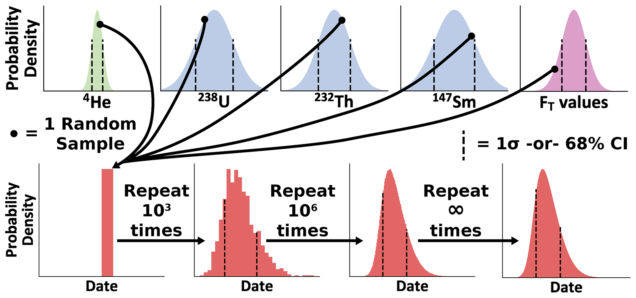
Figure 1A conceptual diagram of Monte Carlo uncertainty modeling for the (U–Th) He system. Each independent Gaussian input probability distribution (with 1σ standard deviation marked as vertical lines) is sampled at random a large number of times. The isotope-specific FT values may also be sampled from multiple distributions, although for illustration only one distribution is shown. Using these randomly sampled inputs, a single date is calculated. This process is repeated until the probability distribution of interest (in this case, a skewed non-Gaussian distribution with the 68 % confidence interval shown with vertical lines) has been sufficiently sampled, as set by the analyst.
The number of Monte Carlo simulations dictates the precision of the results because Monte Carlo analysis is a numerical approximation of uncertainty (e.g., the lower panels in Fig. 1 become progressively smoother with an increasing number of simulations). Therefore, separate from the probability distribution describing date uncertainty, there is a predictable level of variation in uncertainty estimates and other parameters describing the probability distribution (e.g., its mean) given a certain number of total Monte Carlo simulations (Wübbeler et al., 2010). Specifically, the standard error of the standard deviation of a Monte Carlo model is dependent on the uncertainty in the value itself and the number of simulations:
where σμ is the standard deviation of the population mean, σt the date uncertainty estimated by linear uncertainty propagation, and N the number of simulations. To avoid running arbitrary numbers of simulations, we invert this equation to determine the number of iterations required to achieve a user-requested relative precision for the mean:
where N is the number of simulations to run, is the sample mean estimated by calculation of the date using the nominal input values, and p is the user-requested precision in percent uncertainty. By using percent relative uncertainty, the value of the date itself need not be known a priori, as an estimate of the standard deviation of the population mean date can be calculated using the percent relative precision and the date calculation from the input values (Eq. 18).
Table 1Example HeCalc inputsa.

a All values in this table are purely for illustration and do not reflect actual data. b r values are uncertainty covariance as given by their Pearson coefficient (Eq. 19). If no values are provided, uncertainties are assumed to be uncorrelated with r=0.
In this section we describe the implementation of the above methods of date and uncertainty calculation in the new HeCalc software (Martin, 2022). For ease of access and to best provide this software as a resource to the (U–Th) He community, HeCalc is available as both a stand-alone program with a graphical user interface (GUI) and a package in Python 3 available for download from the Python Package Index (PyPI) via pip commands. The descriptions below apply specifically to the GUI version of the software and the main_hecalc function in the Python package; those interested in writing their own code and incorporating the component functions provided in HeCalc may consult the associated documentation for more detailed programming considerations.
4.1 Input
The input for HeCalc is designed to be straightforward and flexible (Table 1). Input files may be in Excel (.xls/.xlsx), comma-separated value (.csv), or tab-delimited text (.txt) format. In addition to data input through a file, HeCalc users may manually input values to calculate a date and uncertainty for a single set of data by clicking on the “Manual” tab. If importing data through a file, the file must contain columns for sample name, U, Th, Sm, He, and all FTs with the headers Sample, mol 238U, mol 232Th, mol 147Sm, mol 4He, 238Ft, 235Ft, 232Ft, and 147Ft (Table 1). Although “mol X” is required as the input column header for U, Th, Sm, and He, the actual units of the input data may be any unit of quantity (e.g., atoms, mol g−1) as long as they are identical. The 1σ uncertainty for each value, in the same units, must be included in the column following each respective value, even if the applied uncertainty is 0 (e.g., for FT values with unknown uncertainty); there is no naming requirement for these headers. If 235U was measured directly, columns for this measurement and its uncertainty should also be present. Correlated uncertainty between the radionuclides and between the isotope-specific FT values can be input using their Pearson correlation coefficient, which is related to the covariance as
where is the covariance between variables a and b. The correlation coefficient is preferable to inputting covariance directly as it has the intuitive meaning of being in the range of [−1, 1], where 1 is perfectly correlated and 0 is fully uncorrelated, while numerical covariance is generally nonintuitive. These values may be included in the input file using headers with the naming convention r 238U–235U and r 238Ft–235Ft (Table 1); either ordering of the correlated uncertainties in the header (i.e., r 238U–235U vs. r 235U–238U) is permitted. Uncertainties are assumed to be uncorrelated unless these columns are explicitly included. Example input files both with and without correlated uncertainty are provided as templates in the code's repository (see the “Code availability” section for a direct link).
Table 2Example HeCalc outputs produced by Table 1 inputs.
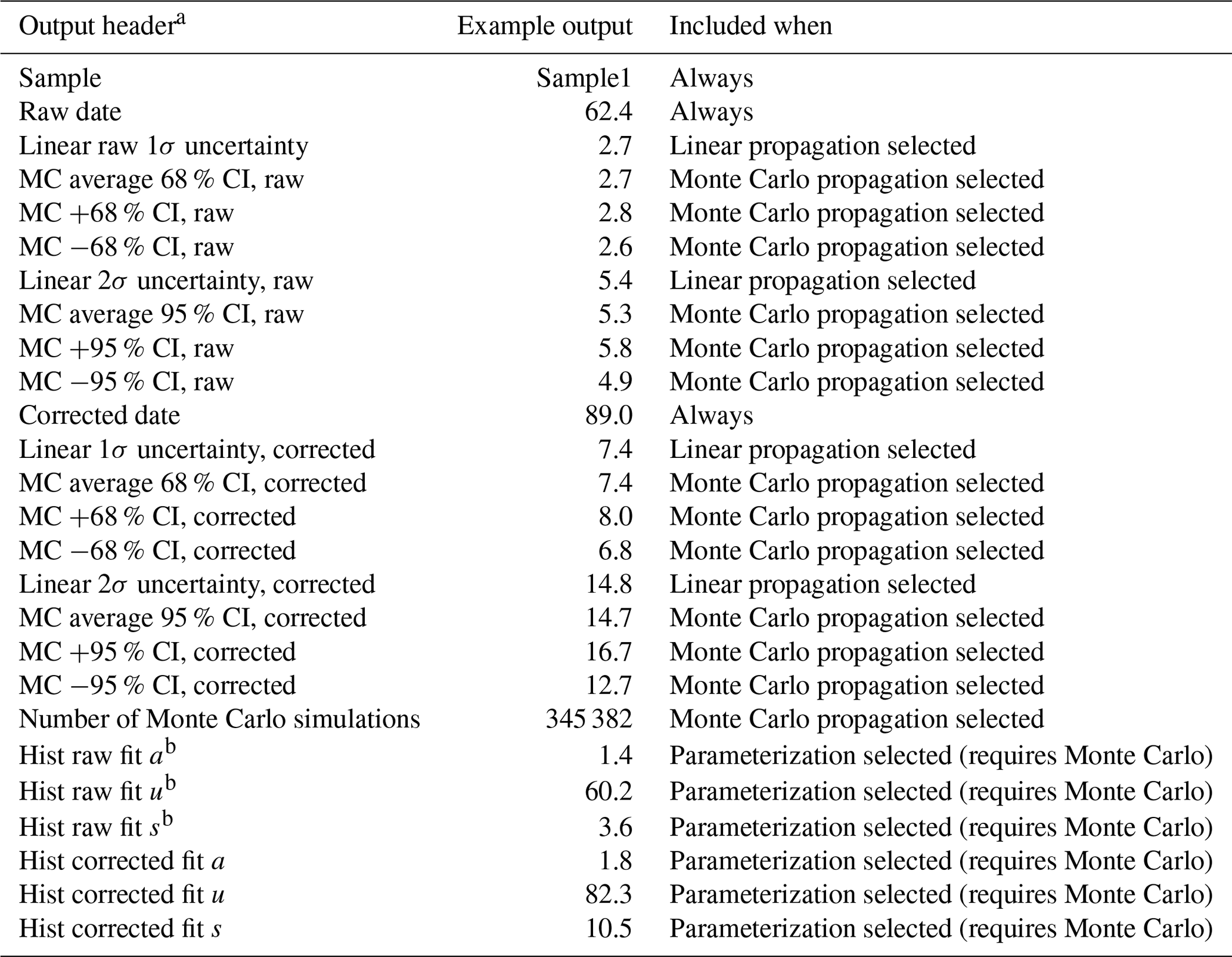
a The header for the file will contain a line for the file path of the input file and (if Monte Carlo propagation is selected) the user-requested precision. b “Hist fit a” refers to the shape or skewness of the histogram. “Hist fit u” is a measure of central tendency of the histogram. “Hist fit s” is a measure of the width of the distribution (Azzalini, 1985; O'Hagan and Leonard, 1976).
The order in which these columns appear is unimportant as long as the uncertainty associated with each value follows that value. Extraneous columns with differing headers also will not interfere with the code's execution. Additionally, if an input Excel file has multiple sheets, the first sheet will be read in by default. If this sheet does not contain the required column headers, the program will ask for the name of the sheet to use instead. In this way, HeCalc ideally allows for input of any given lab's standard data reduction spreadsheet or other typical data product with no or minimal alteration, allowing it to be integrated seamlessly into a lab's existing workflow.
In addition to data input, several further options are provided. The number of decimals included in the output is determined by the user (this option affects only output and does not impact the statistical aspects of the code). The user can also select whether to perform linear uncertainty propagation, Monte Carlo uncertainty propagation, both, or neither. If Monte Carlo uncertainty propagation is selected, the desired precision of the mean is specified in percent as described above. In practice, the precision of the mean date need be no better than the number of significant figures present the in data; for common (U–Th) He analyses, this equates to a precision of ∼ 0.01 %, which generally requires on the order of 104–105 simulations. The program also contains the ability to generate histograms using the Monte Carlo results. If this option is chosen, this histogram may be parameterized as a skew-normal distribution (Azzalini and Capitanio, 1999; O'Hagan and Leonard, 1976).
4.2 Output
There are two main outputs from HeCalc: the results of the date calculation and uncertainty propagation and the histograms of the Monte Carlo results for each sample (Table 2). At a minimum, the sample name, raw date, and corrected date are saved to an Excel sheet titled “Uncertainty Output” that includes a header with the input file's name and directory. The raw and corrected dates in these columns are calculated using each exact input value (e.g., mol 238U = 1 in Table 1); we refer to these dates as “nominal dates” below. The selection of linear uncertainty propagation causes columns to be added titled “Linear raw 1σ uncertainty”, “Linear raw 2σ uncertainty”, “Linear corrected 1σ uncertainty”, and “Linear corrected 2σ uncertainty”, with “raw” indicating no alpha-ejection correction. If Monte Carlo error propagation is selected, a header line specifying the user-requested precision is added, and the columns “MC average 68 % CI, raw”, “MC +68 % CI, raw”, “MC −68 % CI, raw”, “MC average 95 % CI, raw”, “MC +95 % CI, raw”, and “MC −95 % CI, raw”, as well as the corresponding values for FT-corrected dates (titled with “corrected” instead of “raw”) are included along with a column giving the number of Monte Carlo simulations run. The confidence intervals are reported as the 15.865 and 84.135 percentiles (the 68 % confidence interval) and the 2.5 and 97.5 percentiles (the 95 % confidence interval) of the Monte Carlo results, converted to uncertainty values by reference to the nominal date. Throughout this paper, the asymmetry of the confidence intervals will be calculated with respect to the nominal date calculation. It is worth noting that the nominal date does not strictly correspond to the mode of the histogram and instead falls toward the skewed side, meaning that the skew calculations presented here are a slight underestimate of the actual asymmetry in the distribution.
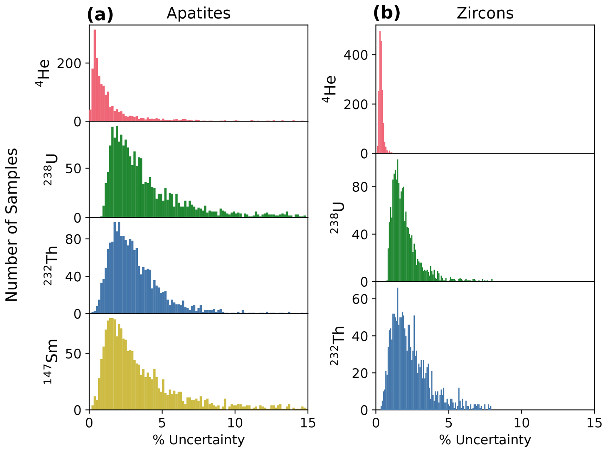
Figure 2Histograms of percent relative uncertainty in 4He, 238U, 232Th, and 147Sm absolute amounts for (a) apatite (N=1978) and (b) zircon (N=1753). Note that the y-axis scales differ for these plots.
If the user chooses to include histograms in the output, an Excel sheet titled “Histogram Output” is added to the workbook, with columns for the center of each histogram bin (i.e., the individual intervals in the histogram) and number of simulations in that bin as x and y values for both the raw and FT-corrected dates. Four total columns are therefore present for each sample. The number of bins is equal to th the number of simulations run or 10 bins, whichever is greater. If parameterization is selected, the histogram is fit to a skew-normal distribution. Although this distribution does not perfectly replicate the histograms generated by HeCalc, it allows for first-order interpretations using continuous probability distributions. Columns are appended to the end of the “Uncertainty Output” sheet titled “Hist raw fit a”, “Hist raw fit u”, and “Hist raw fit s”, as well as the corresponding values for FT-corrected calculations. These parameters correspond to the shape (a, the skewness), location (u, a measure of central tendency), and scale (s, the width of the distribution) parameters for a skew-normal probability distribution function (Azzalini, 1985; O'Hagan and Leonard, 1976).
Here we use the methods described above to calculate the dates and uncertainties for a compilation of real apatite and zircon (U–Th) He data and then examine the overall uncertainty budget and skew in this dataset. In the Appendices we additionally explore the influence of theoretical input uncertainties on date uncertainty, skew in Monte Carlo date distributions, and the differences in dates derived from the linear and Monte Carlo methods (Appendices C–E).
5.1 Uncertainty budget in real data
To assess the uncertainty budget in real (U–Th) He data, we compiled 1978 apatite and 1753 zircon analyses that were acquired with typical and consistent (U–Th) He methods and instrumentation (quadrupole noble gas mass spectrometer and quadrupole ICP-MS) in the University of Colorado Thermochronology Research and Instrumentation Laboratory (CU TRaIL). These data were measured from October 2017 to March 2020 following the methods described in Sturrock et al. (2021) for apatite and Peak et al. (2021) for zircon. Figure 2 shows the histograms of percent relative uncertainty in the absolute amounts of 4He, 238U, 232Th, and (for apatite) 147Sm for this dataset, while Table 3 lists the median value and 68 % confidence interval calculated using the percentile approach (Sect. 3.3) for these distributions. Analytical uncertainties are typically higher for apatites than for zircons due to the lower 4He and radionuclide amounts for apatites relative to zircons, which causes apatite measurements to have lower count rates that are more impacted by blank and background uncertainties. For both apatite and zircon analyses, radionuclide uncertainties are higher than 4He uncertainties. For example, for apatites, the percent uncertainties in 238U, 232Th, and 147Sm amounts are 3.2 %, 2.8 %, and 2.8 %, respectively, which are 3–4 times less precise than the uncertainty in the 4He amount of 0.86 % (Fig. 2a; Table 3). For zircons, the uncertainties of 238U and 232Th are 1.8 % and 2.2 %, respectively, which are 5–6.5 times less precise than the 4He uncertainty of 0.34 % (Fig. 2b, Table 3).
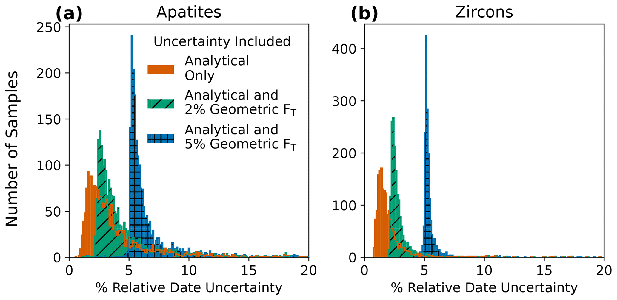
Figure 3Histograms of percent relative uncertainty for corrected (U–Th) He dates for (a) apatite (N=1978) and (b) zircon (N=1753) analyses. Input uncertainties include analytical uncertainties only (4He and radionuclides) and analytical uncertainties propagated with 2 % or 5 % geometric uncertainty in FT, assuming fully correlated individual FT uncertainty values (r=1). Note that the y-axis scales differ for these plots.
Table 3Percent uncertainties in absolute amounts of 4He and radionuclides for apatite and zircon analyses in data compilation.

a Data reported as median and 68 % confidence intervals. b NM: not measured.
We analyze the uncertainty in these data with and without propagating FT uncertainty using HeCalc (Fig. 3). For illustrative purposes, we explored two different scenarios assuming 2 % and 5 % uncertainties in the isotope-specific FT values and fully correlated FT uncertainties. These uncertainties are based on those reported by Zeigler et al. (2022), who found that the FT uncertainty depends partly on grain geometry. Figure 3 shows the distributions of percent relative uncertainty calculated by the Monte Carlo method for the apatite and zircon corrected (U–Th) He dates. Table 4 lists the median value and 68 % confidence interval for these distributions. Propagating only analytical uncertainties (in radionuclides and 4He) yields median date uncertainties of 2.9 % and 1.7 % for apatite and zircon, respectively. With uncertainty in FT included, the date uncertainty increases substantially. For apatites, the uncertainty value increases to 3.5 % and 5.8 %, respectively, when FT uncertainties of 2 % or 5 % are also propagated. For zircons, the uncertainty increases to 2.6 % and 5.2 %, respectively. The addition of FT uncertainty most heavily impacts the analyses with more precise radionuclide and 4He measurements because FT uncertainty comprises a correspondingly larger proportion of the uncertainty budget. Given that FT geometric uncertainty estimates are of the same order of magnitude as – and in some cases larger than – typical analytical uncertainties in (U–Th) He dating, additional efforts to constrain FT uncertainty are important to rigorously calculate uncertainties in individual (U–Th) He dates.
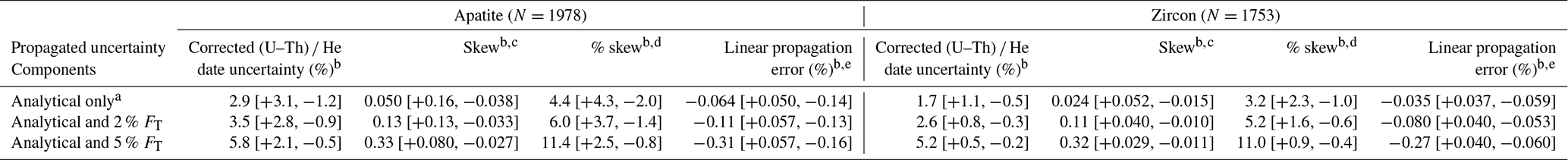
Table 4Percent uncertainty in corrected (U–Th) He dates, skew and percent skew of Monte Carlo-generated date distributions, and percent error in linear propagation method for apatite and zircon analyses in data compilation.
a Analytical refers to uncertainties in 4He and radionuclides. b Data reported as median and 68 % confidence intervals. c Skew of the distribution reported in accordance with its standard unitless definition. d Percent skew is defined here as percent difference between the positive and negative 68 % confidence intervals relative to the date to convey a more intuitive sense of distribution asymmetry. e Percent difference between uncertainty derived from linear uncertainty propagation and averaged 68 % confidence intervals from Monte Carlo uncertainty propagation.
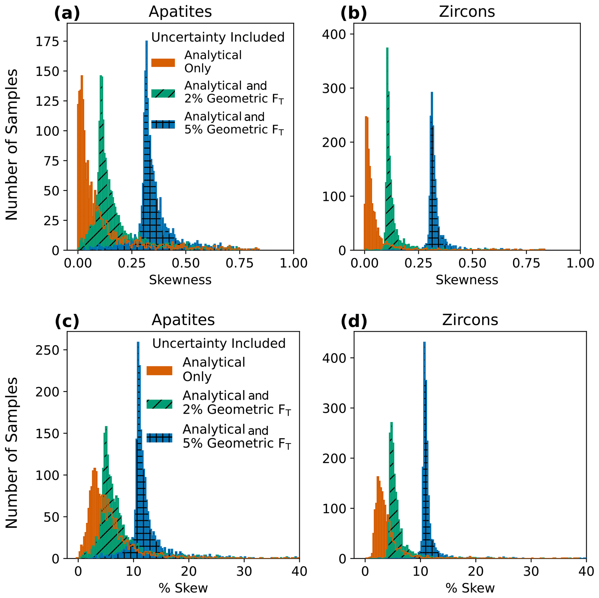
Figure 4Histograms of skew for (a) apatite (N=1978) and (b) zircon (N=1753) analyses. Panels (c) and (d) are the same data but plotted as percent skew, or the percent asymmetry in the 68 % confidence intervals, to aid in more intuitive understanding of the outcomes. Input uncertainties include analytical uncertainty only (4He and radionuclides) and analytical uncertainties propagated with 2 % or 5 % geometric uncertainty in FT, assuming fully correlated individual FT uncertainty values (r=1). Note that the y-axis scales differ between the two plots.
5.2 Skew in real data
We also analyze the compilation of real data in Fig. 2 for skew in Monte Carlo-generated date probability distributions (i.e., asymmetric uncertainty). Skew refers to the extent of asymmetry in the “tails” of a distribution (Figs. 1, D1). “Skewness” is a statistical concept that strictly refers to the third standardized moment of a population, which is a unitless and generally nonintuitive metric. Here we additionally report a percent skew to more intuitively convey the distribution asymmetry, calculated by taking the percent difference between the positive and negative 68 % confidence intervals with respect to the date. This asymmetry would most accurately be reported as separate positive and negative uncertainty values referring to the 68 % confidence interval rather than the more typical 1σ uncertainty reporting of symmetric uncertainty. As an example, for 10 % skew, a 100 ± 6.4 Ma date would be represented as 100 [+6.7, −6.1] Ma at the 1s level.
In our data compilation, positive skew is common and can be significant (Table 3). This is consistent with analysis of theoretical data revealing that skew increases with relative input uncertainty and varies with age (Appendix D; Figs. D1–D3). For the real dataset, with only analytical uncertainty included, the median skew in apatites and zircons is 0.050 and 0.020 (or 4.4 % and 3.2 % skew), respectively. The inclusion of FT uncertainty increases the skew (Fig. 4a–b, Table 4). For apatites, skew rises to 0.13 and 0.33 (or 6.0 % and 11.4 % skew) for 2 % and 5 % uncertainty in FT, respectively (Fig. 4a, Table 4). For zircons, the same combinations of uncertainty yield skews of 0.11 and 0.32 (or 5.2 % and 11 % skew; Fig. 4b, Table 4). For a 2 % FT uncertainty, ∼ 17 % of apatite data and ∼ 6 % of zircon data have a skewness of 0.25 or greater.
General practice in (U–Th) He dating has been to report symmetric uncertainties. Our analysis reveals that for most cases this is appropriate, and averaging asymmetric uncertainties in data reporting is unlikely to substantially impact interpretations. However, for highly asymmetric uncertainties, it may be appropriate to report positive and negative uncertainties separately and only combine the reported uncertainties if they are indistinguishable within the appropriate number of significant figures. Our results suggest that skew may be an important consideration when interpreting (U–Th) He data with less precise 4He and radionuclide measurements because these data generally have date uncertainties with greater skew. In these cases, asymmetric uncertainties may be important for determining whether a dataset is consistent with a given hypothesis within uncertainty. However, a challenge to interpreting dates with asymmetric uncertainties is that no widely used inverse thermal history modeling software for (U–Th) He data permits asymmetric uncertainty input. Future work implementing skewed probability distributions in such software may enhance interpretation of the subset of (U–Th) He data characterized by highly skewed uncertainties.

Figure 5Histograms of the percent difference between averaged Monte Carlo-derived confidence intervals and linear uncertainty propagation for (a) apatite (N=1978) and (b) zircon (N=1753) analyses. Input uncertainties include analytical uncertainty only (4He and radionuclides) and analytical uncertainties propagated with 2 % or 5 % geometric uncertainty in FT, assuming fully correlated individual FT uncertainty values (r=1). The outlines of covered histograms are included to show detail for each.
5.3 Comparison of linear and Monte Carlo uncertainty propagation results for real data
Finally, we compare the uncertainties derived from linear uncertainty propagation with the averaged 68 % confidence intervals from Monte Carlo propagation for the compiled dataset. For nearly all analyses, the uncertainties yielded by the two methods are within 1 % of each other, regardless of the amount of FT uncertainty included (Fig. 5a, Table 4). Thus, error due to linear uncertainty propagation (i.e., inaccurately calculated uncertainty resulting from an assumption of linearity) is largely insignificant in this dataset, and the uncertainties yielded by the two methods are interchangeable in most circumstances. In contrast, skew, discussed in the previous section, is only revealed by the Monte Carlo method using the equations presented here and included in the HeCalc software. The asymmetric uncertainties of some samples, specifically those with atypically large input uncertainties, are more important for accurate uncertainty analysis than error introduced in the uncertainty calculation due to linear uncertainty propagation.
Here we publish fully traceable end-to-end calculations of uncertainty in (U–Th) He dates, including the propagation of uncertainties in FT values. We also provide a software package, HeCalc, to do these calculations explicitly and to perform more accurate Monte Carlo propagation of these uncertainties. Using a compilation of apatite and zircon (U–Th) He analyses, we find that for a common instrumental setup (quadrupole noble gas and ICP mass spectrometers), uncertainty in radionuclide quantification is generally 3–6.5 times larger than the uncertainty in 4He measurement. When only 4He and radionuclide uncertainties are propagated, the typical alpha-ejection-corrected (U–Th) He date uncertainty is 2.9 % for apatites and 1.7 % for zircons. The inclusion of 2 % and 5 % geometric uncertainty in the FT values yields greater date uncertainty of 3.5 % and 5.8 % for apatites and 2.6 % and 5.2 % for zircons.
For the compiled dataset, the asymmetry in the 68 % confidence interval can be significant, especially for dates with less precise input uncertainty. With 2 % uncertainty included in FT, 17 % of all apatite and 6 % of all zircon analyses have skewness greater than 0.25. The results of linear uncertainty propagation for these data agree with those from Monte Carlo uncertainty propagation to within ∼ 1 %, indicating that this error is negligible. Given that Monte Carlo uncertainty propagation permits calculation of skewed probability distributions and does not make an assumption of linearity in the (U–Th) He age equation, we propose that this method should be preferred for uncertainty calculation in (U–Th) He data. However, the current lack of a means of including asymmetric uncertainty in thermal history modeling, as well as the roughly equivalent symmetric uncertainty values from Monte Carlo and linear uncertainty propagation methods, indicates that the results are likely interchangeable for common workflows, pending advancements in the (U–Th) He method and interpretive models.
The methods presented here allow for more rigorous inter-laboratory data comparisons and retrospective data analyses by providing a consistent means of quantifying the uncertainty budget of a given (U–Th) He analysis. Further developments of the (U–Th) He technique are also facilitated by this study. In particular, this work both suggests that continued refinement of FT uncertainty is warranted and provides a framework into which those developments may be placed. Using the Monte Carlo results, asymmetric uncertainty may also be quantified and could potentially be included in future versions of thermal history modeling software. Finally, fully accounting for analytical and geometric uncertainties will better isolate the magnitude of over-dispersion and promote more effective examination of its causes.
Here we provide a set of equations that allows for propagation of directly quantified of 235U uncertainty.
The summation terms in Eqs. (A1) and (A2) differ from Eq. (15) because 235U is directly quantified as follows.
Finally, with 235U quantified directly, the overall uncertainty propagation equation becomes the following.
Negative dates are permitted in the probability distributions produced by HeCalc; this is because the input distributions are presumed to be Gaussian, meaning that if the input variables have high relative errors, negative molar amounts of U, Th, Sm, and He are possible. This behavior is formally correct for Gaussian uncertainties, albeit nonphysical. For low count rates associated with high relative uncertainty, a Poisson distribution (rather than Gaussian distribution) is appropriate and would prevent negative input values. However, high relative input uncertainties are generally due to a measurement being near or below background rather than low count rates for which the underlying poisson distribution of the data is not well-approximated by a Gaussian. As a result, there are potential instances of negative molar amounts included in the Monte Carlo calculations. In some rare instances when a negative amount of a given parent nuclide is produced in the generation of random data, the (U–Th) He date equation may have multiple or no solutions. In these cases, the result is simply removed from the sample of calculated ages. The total number of such removals is tracked, and if the proportion removed exceeds the requested precision level, all results associated with the Monte Carlo simulation are reported as NaN (i.e., “not a number”) and only the linear uncertainty propagation results are returned. For typical inputs of routine analyses with a few percent relative uncertainty (Sect. 5), the impact of this phenomenon is negligible.
We examined the overall behavior of date uncertainty from 0 to 4.6 Ga as a function of relative input uncertainties of 1 %, 5 %, and 20 % for 4He (Fig. C1a), radionuclides (Fig. C1b), and isotope-specific FT values (Fig. C1c). This range of dates was generated by fixing the 238U and 232Th values while varying 4He values (no 147Sm was included because of its generally negligible influence on apatite and zircon results). Th U ratios representative of a typical zircon (based on the Fish Canyon Tuff zircon reference standard), a typical apatite (from a compilation of apatite data; Sect. 5), and the Durango apatite reference standard (0.6, 1.25, and 16.1, respectively) were used. For all calculations, an isotope-specific FT value of 0.7 was applied to all isotopes to permit comparisons between raw and FT-corrected dates (while isotope-specific values will differ in real data, we simplify these to a single value here). We initially explored the influence of individual uncertainties on the date by varying the relative uncertainty of one input parameter (4He, radionuclides, or FT) while fixing all other uncertainties at 0 (Fig. C1). We then evaluated how combinations of input uncertainties can influence the date (Fig. C2), although this is more fully evaluated in practical terms using real data, as in Sect. 5. For these exercises, we use the results from Monte Carlo uncertainty propagation, as this technique is in theory fully accurate (see Appendix E for further discussion). We used a constant number of simulations set at 108 to provide precise estimates of skew and comparisons between the Monte Carlo and linear uncertainty propagation methods. This number of simulations corresponds to a minimum precision of the mean date of ∼ 0.0002 % (2 µg g−1).
For individual input uncertainties, at young dates the input and output relative uncertainties are similar. If all uncertainty is in the 4He value or correlated FT values, the relative date uncertainty is equivalent to the input uncertainty at zero age (Fig. C1a, c). For uncertainty in the radionuclides, the relative date uncertainty at zero age is approximately 80 % of the magnitude of the relative input uncertainty (a 4:5 ratio). The exact scaling between input and output uncertainties is dependent on the Th U ratio (Fig. C1b, c).
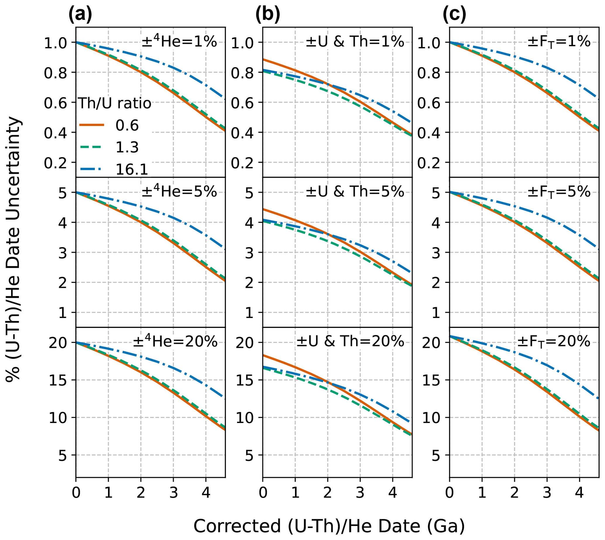
Figure C1Corrected (U–Th) He date uncertainties for dates of 0 to 4.6 Ga with input uncertainty in only one parameter and all others held at zero. Plots of percent relative uncertainty of the corrected date vs. corrected date for uncertainty only in (a) 4He, (b) radionuclides, and (c) uncertainties only in FT, with fully correlated FT uncertainties (r=1). Input uncertainties of 1 % (top panels), 5 % (middle panels), and 20 % (bottom panels) are applied. The two 68 % confidence intervals of the distributions resulting from Monte Carlo simulation were averaged to derive an equivalent 1σ uncertainty. The line colors correspond to the Th U ratio for typical zircon (0.61, derived from the Fish Canyon Tuff zircon reference standard), for typical apatite (1.25, derived from apatite data compilation), and for the Durango apatite reference standard (16.1).

Figure C2Corrected (U–Th) He date uncertainties for dates of 0 to 4.6 Ga with uncertainty in multiple input parameters. Plots of percent relative uncertainty in the corrected date vs. corrected date for the combination of (a) 1 % uncertainty and (b) 5 % uncertainty in 4He and radionuclides, as well as additionally in the isotope-specific FT values. Calculations assume fully correlated uncertainty in isotope-specific FT values (r=1) for a Th U ratio of 1.3 (derived from the Fish Canyon Tuff zircon reference standard).
The relative date uncertainty decreases with increasing absolute date for constant relative input uncertainties. For example, while uncertainty in 4He has a one-to-one relationship with date uncertainty at zero age, at 4.6 Ga the date uncertainty is approximately half that of the input 4He uncertainty (Fig. C1a). The same phenomenon is observed for uncertainty in radionuclides and FT (Fig. C1b, c). The relative extent of decreasing uncertainty as a function of increasing date is dependent on Th U ratio and is independent of the magnitude of input uncertainty (i.e., the three vertically stacked panels in Figs. C1a, 3b, and c are identical aside from the scale of their y axes).
Decreasing uncertainty with increasing date is also observed for multiple input uncertainties. Figure C2 illustrates examples of combining uncertainties with differing magnitudes in quadrature. At zero age, the uncertainty in the date introduced by each input parameter combines roughly in quadrature to provide the uncertainty in the date. For example, at zero age, a 5 % uncertainty in all parameters (4He, radionuclides, correlated FT uncertainty), each of which alone introduces a date uncertainty of 5 %, 4 %, and 5 %, respectively, together yields a date uncertainty of 8.1 % (; solid line, Fig. C2b). Alternatively, if input uncertainties have highly differing magnitudes, the larger uncertainty will dominate and the resulting combined uncertainty will be approximately equal to the larger uncertainty. As an example, a 10 % and 1 % uncertainty combined in quadrature will result a 10.05 % uncertainty. This behavior suggests that reducing the magnitude of the largest input uncertainty will be the most effective means of reducing overall date uncertainty.
The magnitude of skew correlates directly with the magnitude of input uncertainty (Figs. D1–D2). For low percent input uncertainties in all parameters, the magnitude of skew is low. For example, uncertainties of 1 % for all inputs yield 0.06 skewness for dates from 0 to 4.6 Ga (Fig. D2a–c, top panels). Only when the input uncertainties are larger does the effect of skew on the dates become substantial (Fig. D2a–c, middle and bottom panels). In the case of larger uncertainty in 4He (Fig. D2a, middle and bottom panels), skew increases from zero to progressively larger negative values at older dates. The inverse is true for uncertainty in the radionuclides and FT; skew is highest when uncertainty in these parameters is high for young dates and decreases with increasing age (Fig. D2b–c, middle and bottom panels). Note that although asymmetric uncertainties as high as a skewness of 0.85 can be yielded by radionuclide uncertainties of 20 %, such large uncertainties are anomalous and do not typify most high-quality (U–Th) He datasets (Sect. 5).
When uncertainty is included in multiple input parameters, the overall skew is a combination of the skew resulting from individual input uncertainties (Fig. D3). Unlike date uncertainty, which combines individual inputs in quadrature, the combination of skew from individual inputs does not follow an easily predictable trend.
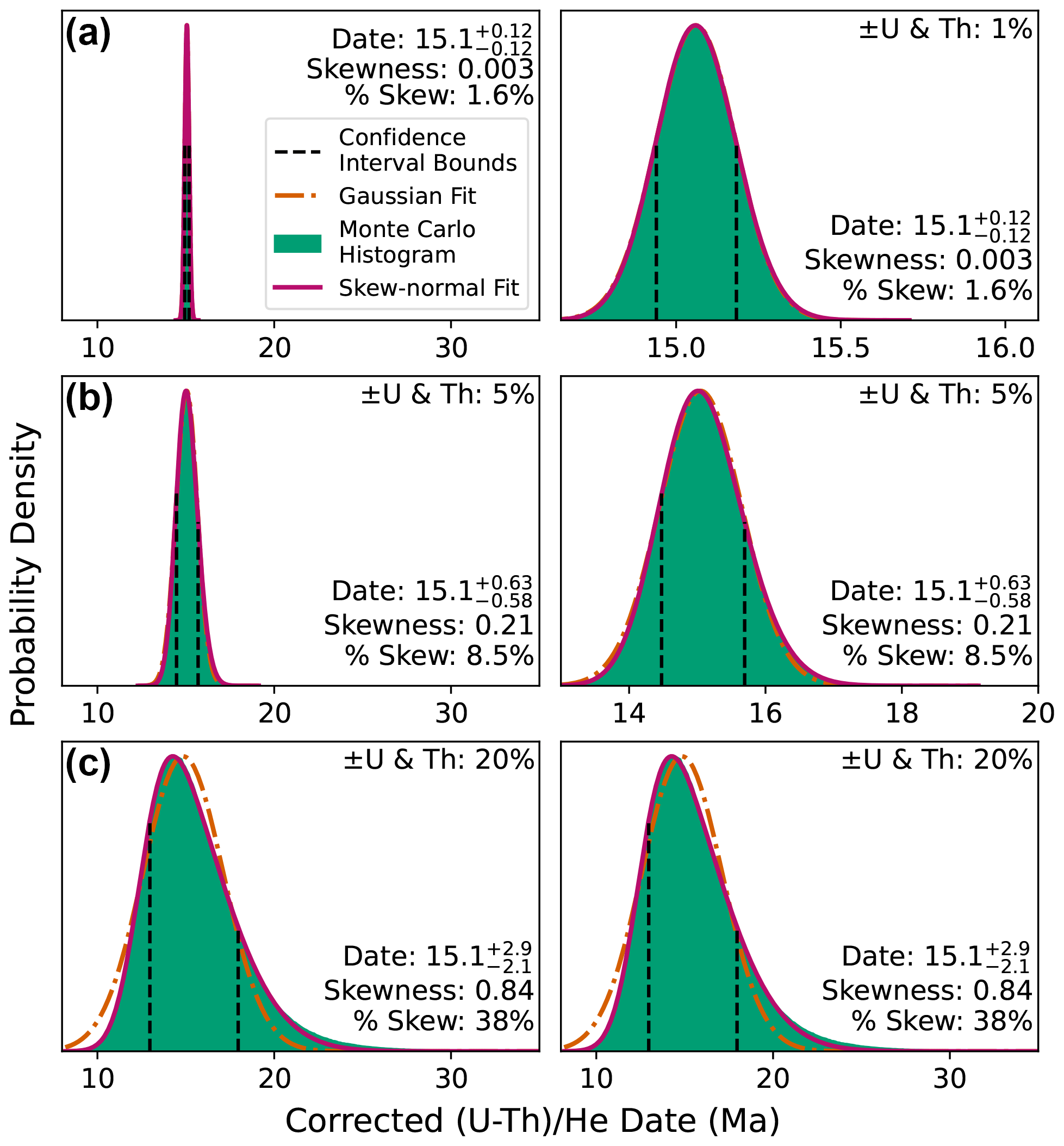
Figure D1An illustration of how differing uncertainty affects the skew of date probability distributions for inputs yielding a date of 15.1 Ma (assuming a typical apatite Th U ratio of 0.61). (a) Low radionuclide uncertainty of 1 %, giving a skewness of 0.003; (b) high radionuclide uncertainty of 5 %, giving a skewness of 0.21; and (c) extremely high radionuclide uncertainty of 20 % (see discussion of real data in Sect. 5), giving skewness of 0.84. The Gaussian fits in panels (a) and (b) are almost entirely concealed by the skew-normal fit plotted above it. The left column shows all distributions at the same scale, while the right-hand column zooms into the more precise (and less skewed) distributions to show detail.
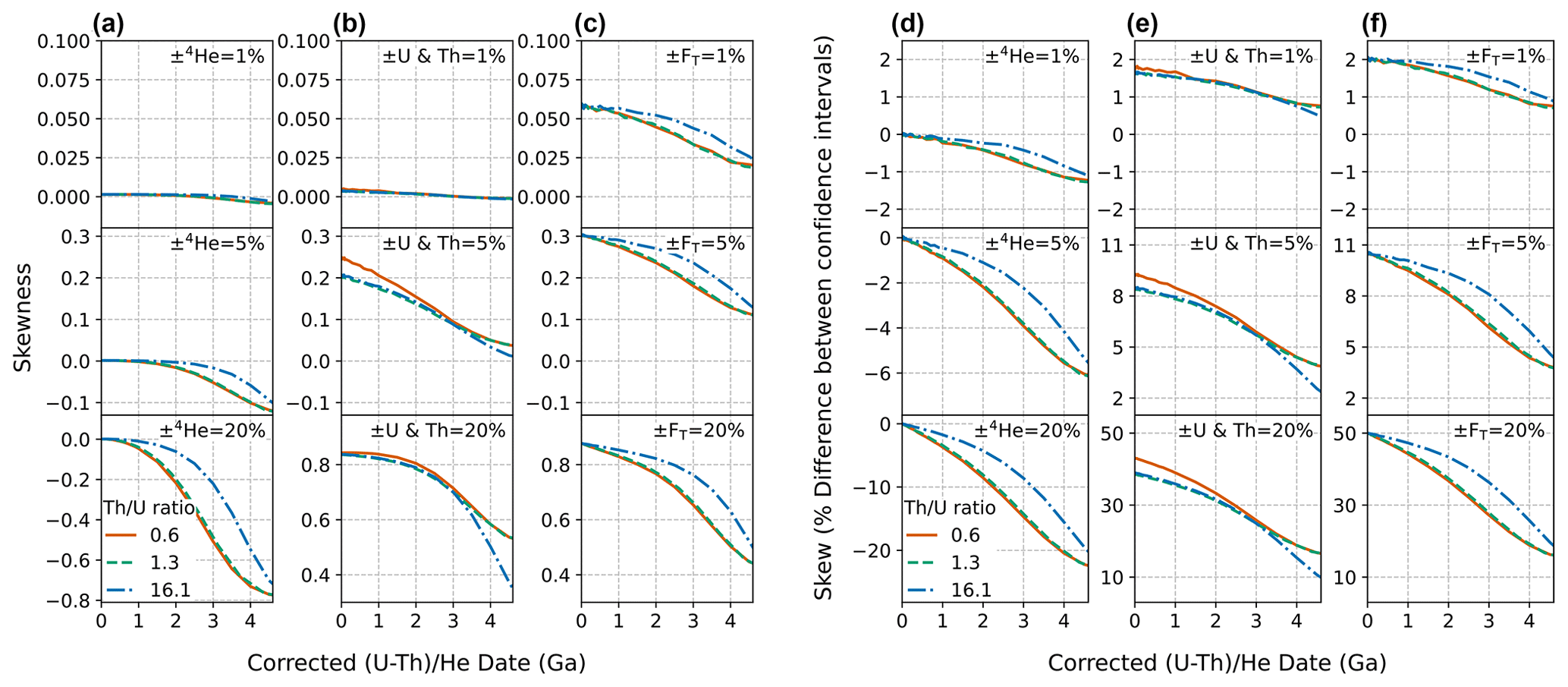
Figure D2Skew for dates from 0 to 4.6 Ga with input uncertainty in only one parameter and all others held at zero. (a) 4He, (b) radionuclides, and (c) uncertainties only in FT, with fully correlated FT uncertainties. Panels (d)–(f) are the same data but plotted as percent skew, or the percent asymmetry in the 68 % confidence intervals, to aid in more intuitive understanding of the outcomes. Input uncertainties of 1 % (top panels), 5 % (middle panels), and 20 % (bottom panels) are applied. The two 68 % confidence intervals of the distributions from the Monte Carlo simulation were averaged to derive an equivalent 1σ uncertainty. The line colors correspond to the Th U ratio for typical zircon (0.61, derived from the Fish Canyon Tuff zircon reference standard), for typical apatite (1.25, derived from apatite data compilation), and for the Durango apatite reference standard (16.1). Note that the y-axis scale is different for some panels.
To compare linear and Monte Carlo error propagation derived uncertainties, we average the two 68 % confidence intervals to determine uncertainty from both methods at the 1σ level. For data with high skew, this method provides a means of comparing the scale of these two differing output distributions directly. The magnitude of the error in uncertainty estimation from linear uncertainty propagation due to nonlinearity in the date equation is proportional to the magnitude of the input uncertainties. As shown in Fig. E1a, for uncertainty in He alone, the Monte Carlo and linear methods yield identical results at younger dates, with linear uncertainty propagation beginning to underestimate the true uncertainty values at older dates as the absolute magnitude of 4He uncertainty increases (reaching a maximum discrepancy of ∼ 2 % for input uncertainties of 20 % at 4.6 Ga). Uncertainty in radionuclides and FT have the opposite effect; the discrepancy between the Monte Carlo and linear methods is greatest (∼ 3 % for input uncertainties of 20 %, dependent on Th U ratio and correlation in FT uncertainties) at zero age and decreases with increasing date. This small extent of error indicates that Monte Carlo and linear methods are in general agreement.
As linear uncertainty propagation relies on an arithmetic calculation rather than random sampling, this method provides predictable and repeatable results for uncertainty calculations and is amenable to encoding in spreadsheet programs, facilitating the inclusion of the equations provided in Sect. 3.2 in existing spreadsheet-based workflows. However, the presence of skew in (U–Th) He date uncertainties and the inaccuracies in uncertainty calculation induced by nonlinearity in the (U–Th) He age equation indicate that the more accurate Monte Carlo uncertainty propagation method is more universally applicable. Although in the past computational (in)efficiency was generally considered the weakness of Monte Carlo methods, running as many as 1 million Monte Carlo simulations in HeCalc takes less than 1 s on a modern computer for a typical sample. This number of random samples provides a sufficiently large population that output histograms are relatively smooth, yielding accurate uncertainty calculations with sufficient significant figures that the model-to-model variation induced by random sampling is negligible. As the Monte Carlo method in HeCalc is not excessively computationally intensive and provides both skew and accurate uncertainties, we suggest that the Monte Carlo method is preferable to linear uncertainty propagation in the (U–Th) He system.
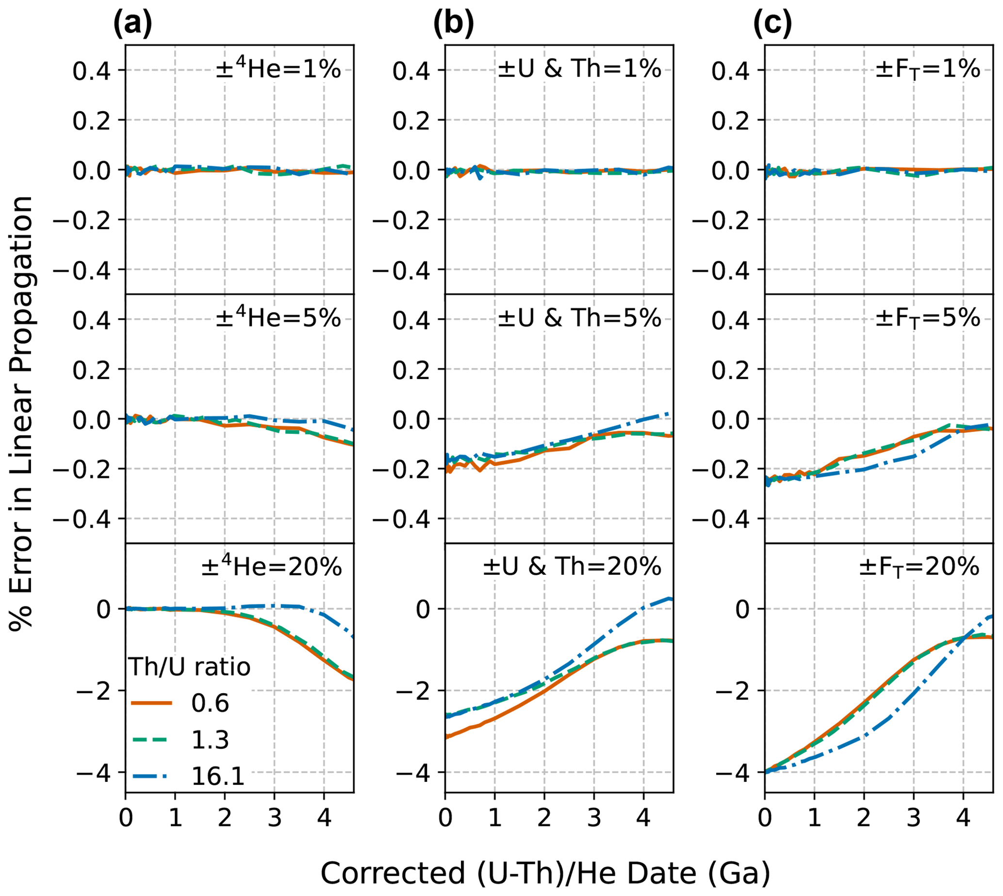
Figure E1The percent error introduced by using linear uncertainty propagation instead of Monte Carlo uncertainty propagation for dates from 0 to 4.6 Ga. Plots of percent difference between the Monte Carlo and linear uncertainty propagation results vs. corrected date for uncertainty only in (a) 4He, (b) radionuclides, and (c) FT, assuming fully correlated FT uncertainties.The two 68 % confidence intervals of the distributions from the Monte Carlo simulation were averaged to derive an equivalent 1 s uncertainty. Relative input uncertainties of 1 % (top panels), 5 % (middle panels), and 20 % (bottom panels) were applied. The line colors correspond to the Th U ratio for typical zircon (0.61, derived from the Fish Canyon Tuff zircon reference standard), for typical apatite (1.25, derived from apatite data compilation), and for the Durango apatite reference standard (16.1).
Version 1.0.1 of the HeCalc software is available at https://doi.org/10.5281/zenodo.7453426 (Martin, 2022). A Windows-executable application to run HeCalc is available through the latest release on the software's GitHub repository at https://github.com/Peter-E-Martin/HeCalc/releases/latest (last access: 25 January 2023).
The data used in this paper are from an anonymized compilation of samples run in the CU TRaIL at the University of Colorado Boulder. These data are dominated by independent contract samples and are published at the discretion of the individuals who paid for the analyses.
PEM, RMF, and JRM conceptualized the project; JRM curated the data; PEM performed the formal analyses; RMF and JRM acquired funding; PEM, RMF, and JRM performed the investigation; PEM developed the methodology and wrote the software; RMF provided supervision; PEM wrote the original draft, and RMF and JRM reviewed and edited the paper.
The contact author has declared that none of the authors has any competing interests.
Publisher's note: Copernicus Publications remains neutral with regard to jurisdictional claims in published maps and institutional affiliations.
We thank Noah McLean for numerous and very helpful discussions while developing HeCalc and writing this paper. HeCalc and this paper were greatly improved following discussions at the 17th International Conference on Thermochronology, in particular with Danny Stockli, Florian Hoffman, Marissa Tremblay, and Kip Hodges. We appreciate helpful reviews by Ryan Ickert and an anonymous reviewer that helped to clarify and streamline this paper. The (U–Th) He analyses used in the data compilation presented here were generated by instrumentation funded by National Science Foundation award EAR-1126991 to Flowers and awards EAR-1559306 and EAR-1920648 to Flowers and Metcalf.
This research has been supported by the National Science Foundation (grant nos. EAR-1126991, EAR-1559306, and EAR-1920648).
This paper was edited by Brenhin Keller and reviewed by Ryan Ickert and one anonymous referee.
Anderson, G. M.: Error propagation by the Monte Carlo method in geochemical calculations, Geochim. Cosmochim. Ac., 40, 1533–1538, https://doi.org/10.1016/0016-7037(76)90092-2, 1976.
Azzalini, A.: A Class of Distributions Which Includes the Normal Ones, Scand. J. Stat., 12, 171–178, 1985.
Azzalini, A. and Capitanio, A.: Statistical applications of the multivariate skew normal distribution, J. Roy. Stat. Soc. Ser. B, 61, 579–602, https://doi.org/10.1111/1467-9868.00194, 1999.
Bevington, P. and Robinson, D. K.: Data Reduction and Error Analysis for the Physical Sciences, 3rd Edn., McGraw-Hill Education, 344 pp., ISBN 13: 9780071199261, 2003.
Brown, R. W., Beucher, R., Roper, S., Persano, C., Stuart, F., and Fitzgerald, P.: Natural age dispersion arising from the analysis of broken crystals, Part I: Theoretical basis and implications for the apatite (U–Th) He thermochronometer, Geochim. Cosmochim. Ac., 122, 478–497, https://doi.org/10.1016/j.gca.2013.05.041, 2013.
Cooperdock, E. H. G., Ketcham, R. A., and Stockli, D. F.: Resolving the effects of 2-D versus 3-D grain measurements on apatite (U–Th) thinsp;He age data and reproducibility, Geochronology, 1, 17–41, https://doi.org/10.5194/gchron-1-17-2019, 2019.
Evans, N. J., McInnes, B. I. A., Squelch, A. P., Austin, P. J., McDonald, B. J., and Wu, Q.: Application of X-ray micro-computed tomography in (U–Th) He thermochronology, Chem. Geol., 257, 101–113, https://doi.org/10.1016/j.chemgeo.2008.08.021, 2008.
Farley, K. A., Wolf, R. A., and Silver, L. T.: The effects of long alpha-stopping distances on (U–Th) He ages, Geochim. Cosmochim. Ac., 60, 4223–4229, https://doi.org/10.1016/S0016-7037(96)00193-7, 1996.
Farley, K. A., Shuster, D. L., and Ketcham, R. A.: U and Th zonation in apatite observed by laser ablation ICPMS, and implications for the (U–Th) He system, Geochim. Cosmochim. Ac., 75, 4515–4530, https://doi.org/10.1016/j.gca.2011.05.020, 2011.
Fitzgerald, P. G., Baldwin, S. L., Webb, L. E., and O'Sullivan, P. B.: Interpretation of (U–Th) He single grain ages from slowly cooled crustal terranes: A case study from the Transantarctic Mountains of southern Victoria Land, Chem. Geol., 225, 91–120, https://doi.org/10.1016/j.chemgeo.2005.09.001, 2006.
Flowers, R. M., Ketcham, R. A., Shuster, D. L., and Farley, K. A.: Apatite (U–Th) He thermochronometry using a radiation damage accumulation and annealing model, Geochim. Cosmochim. Ac., 73, 2347–2365, https://doi.org/10.1016/j.gca.2009.01.015, 2009.
Flowers, R. M., Zeitler, P. K., Danišík, M., Reiners, P. W., Gautheron, C., Ketcham, R. A., Metcalf, J. R., Stockli, D. F., Enkelmann, E., and Brown, R. W.: (U-Th) = He chronology: Part 1. Data, uncertainty, and reporting, GSA Bull., 30, https://doi.org/10.1130/B36266.1, 2022.
Flowers, R. M., Zeitler, P. K., Danišík, M., Reiners, P. W., Gautheron, C., Ketcham, R. A., Metcalf, J. R., Stockli, D. F., Enkelmann, E., and Brown, R. W.: (U-Th) He chronology: Part 1. Data, uncertainty, and reporting, GSA Bull., 135, 104–136, https://doi.org/10.1130/B36266.1, 2022b.
Gallagher, K.: Transdimensional inverse thermal history modeling for quantitative thermochronology, J. Geophys. Res.-Sol. Ea., 117, B02408, https://doi.org/10.1029/2011JB008825, 2012.
Gautheron, C., Tassan-Got, L., Barbarand, J., and Pagel, M.: Effect of alpha-damage annealing on apatite (U–Th) He thermochronology, Chem. Geol., 266, 157–170, https://doi.org/10.1016/j.chemgeo.2009.06.001, 2009.
Glotzbach, C., Lang, K. A., Avdievitch, N. N., and Ehlers, T. A.: Increasing the accuracy of (U-Th(-Sm)) He dating with 3D grain modelling, Chem. Geol., 506, 113–125, https://doi.org/10.1016/j.chemgeo.2018.12.032, 2019.
Guenthner, W. R., Reiners, P. W., Ketcham, R. A., Nasdala, L., and Giester, G.: Helium diffusion in natural zircon: Radiation damage, anisotropy, and the interpretation of zircon (U-Th) He thermochronology, Am. J. Sci., 313, 145–198, https://doi.org/10.2475/03.2013.01, 2013.
Herman, F., Braun, J., Senden, T. J., and Dunlap, W. J.: (U–Th) He thermochronometry: Mapping 3D geometry using micro-X-ray tomography and solving the associated production–diffusion equation, Chem. Geol., 242, 126–136, https://doi.org/10.1016/j.chemgeo.2007.03.009, 2007.
Hiess, J., Condon, D. J., McLean, N., and Noble, S. R.: 238U 235U Systematics in Terrestrial Uranium-Bearing Minerals, Science, 335, 1610–1614, https://doi.org/10.1126/science.1215507, 2012.
Hourigan, J. K., Reiners, P. W., and Brandon, M. T.: U-Th zonation-dependent alpha-ejection in (U-Th) He chronometry, Geochim. Cosmochim. Ac., 69, 3349–3365, https://doi.org/10.1016/j.gca.2005.01.024, 2005.
House, M. A., Farley, K. A., and Stockli, D.: Helium chronometry of apatite and titanite using Nd-YAG laser heating, Earth Pl. Sc. Lett., 183, 365–368, https://doi.org/10.1016/S0012-821X(00)00286-7, 2000.
Johnstone, S., Hourigan, J., and Gallagher, C.: LA-ICP-MS depth profile analysis of apatite: Protocol and implications for (U–Th) He thermochronometry, Geochim. Cosmochim. Ac., 109, 143–161, https://doi.org/10.1016/j.gca.2013.01.004, 2013.
Ketcham, R. A.: Forward and Inverse Modeling of Low-Temperature Thermochronometry Data, Rev. Mineral. Geochem., 58, 275–314, https://doi.org/10.2138/rmg.2005.58.11, 2005.
Ketcham, R. A., Gautheron, C., and Tassan-Got, L.: Accounting for long alpha-particle stopping distances in (U–Th–Sm) He geochronology: Refinement of the baseline case, Geochim. Cosmochim. Ac., 75, 7779–7791, https://doi.org/10.1016/j.gca.2011.10.011, 2011.
Ketcham, R. A., Tremblay, M., Abbey, A., Baughman, J., Cooperdock, E., Jepson, G., Murray, K., Odlum, M., Stanley, J., and Thurston, O.: Report from the 17th International Conference on Thermochronology, Earth Space Sci. Open Ar., 1–20, https://doi.org/10.1002/essoar.10511082.1, 2022.
Martin, P.: HeCalc (1.0.1), Zenodo [code], https://doi.org/10.5281/zenodo.7453426, 2022.
McLean, N. M., Bowring, J. F., and Bowring, S. A.: An algorithm for U-Pb isotope dilution data reduction and uncertainty propagation, Geochem. Geophy. Geosy., 12, Q0AA18, https://doi.org/10.1029/2010GC003478, 2011.
Meesters, A. G. C. A. and Dunai, T. J.: A noniterative solution of the (U-Th) He age equation, Geochem. Geophy. Geosy., 6, Q04002, https://doi.org/10.1029/2004GC000834, 2005.
Murray, K. E., Orme, D. A., and Reiners, P. W.: Effects of U–Th-rich grain boundary phases on apatite helium ages, Chem. Geol., 390, 135–151, https://doi.org/10.1016/j.chemgeo.2014.09.023, 2014.
O'Hagan, A. and Leonard, T.: Bayes estimation subject to uncertainty about parameter constraints, Biometrika, 63, 201–203, https://doi.org/10.1093/biomet/63.1.201, 1976.
Peak, B. A., Flowers, R. M., Macdonald, F. A., and Cottle, J. M.: Zircon (U-Th) He thermochronology reveals pre-Great Unconformity paleotopography in the Grand Canyon region, USA, Geology, 49, 1462–1466, https://doi.org/10.1130/G49116.1, 2021.
Possolo, A. and Iyer, H. K.: Invited Article: Concepts and tools for the evaluation of measurement uncertainty, Rev. Sci. Instrum., 88, 011301, https://doi.org/10.1063/1.4974274, 2017.
Sturrock, C. P., Flowers, R. M., and Macdonald, F. A.: The Late Great Unconformity of the Central Canadian Shield, Geochem. Geophy. Geosy., 22, e2020GC009567, https://doi.org/10.1029/2020GC009567, 2021.
Wernicke, R. S. and Lippolt, H. J.: Dating of vein Specularite using internal (U + Th) 4He isochrons, Geophys. Res. Lett., 21, 345–347, https://doi.org/10.1029/94GL00014, 1994.
Wolf, R. A., Farley, K. A., and Silver, L. T.: Helium diffusion and low-temperature thermochronometry of apatite, Geochim. Cosmochim. Ac., 60, 4231–4240, https://doi.org/10.1016/S0016-7037(96)00192-5, 1996.
Wübbeler, G., Harris, P. M., Cox, M. G., and Elster, C.: A two-stage procedure for determining the number of trials in the application of a Monte Carlo method for uncertainty evaluation, Metrologia, 47, 317–324, https://doi.org/10.1088/0026-1394/47/3/023, 2010.
Zeigler, S. D., Metcalf, J. R., and Flowers, R. M.: A practical method for assigning uncertainty and improving the accuracy of alpha-ejection corrections and eU concentrations in apatite (U-Th) He chronology, EGUsphere [preprint], https://doi.org/10.5194/egusphere-2022-1005, 2022.
Zeitler, P. K., Herczeg, A. L., McDougall, I., and Honda, M.: U-Th-He dating of apatite: A potential thermochronometer, Geochim. Cosmochim. Ac., 51, 2865–2868, https://doi.org/10.1016/0016-7037(87)90164-5, 1987.
Zeitler, P. K., Enkelmann, E., Thomas, J. B., Watson, E. B., Ancuta, L. D., and Idleman, B. D.: Solubility and trapping of helium in apatite, Geochim. Cosmochim. Ac., 209, 1–8, https://doi.org/10.1016/j.gca.2017.03.041, 2017.
- Abstract
- Introduction
- Background: uncertainty components in (U–Th) He dates
- Date and uncertainty calculation methods
- Helium date and uncertainty Calculator (HeCalc) code
- Discussion
- Conclusions
- Appendix A: Additional linear uncertainty propagation equations
- Appendix B: Implications of Gaussian input uncertainties in HeCalc
- Appendix C: Uncertainty in date as a function of input uncertainties
- Appendix D: Skew in distributions yielded by Monte Carlo uncertainty propagation
- Appendix E: Comparison of linear and Monte Carlo uncertainty propagation results
- Code availability
- Data availability
- Author contributions
- Competing interests
- Disclaimer
- Acknowledgements
- Financial support
- Review statement
- References