Towards the construction of regional marine radiocarbon calibration curves: an unsupervised machine learning approach

Radiocarbon may serve as a powerful dating tool in palaeoceanography, but its accuracy is limited by the need to calibrate radiocarbon dates to calendar ages. A key problem is that marine radiocarbon dates must be corrected for past offsets from either the contemporary atmosphere (i.e. “reservoir age” offsets) or a modelled estimate of the global average surface ocean (i.e. delta-R offsets). This presents a challenge because the spatial distribution of reservoir ages and delta-R offsets can vary significantly, particularly over periods of major marine hydrographic and/or carbon cycle change such as the last deglaciation. Modern reservoir age and delta-R estimates therefore have limited applicability. While forward modelling of past R-age variability has been proposed as a means of resolving this problem, this requires accurate a priori knowledge of past global radiocarbon budget closure (i.e. production, and cycling), which we currently lack. In this context, the construction of empirical regional marine calibration curves could provide a way forward. However, the spatial reach of such calibrations and their robustness subject to (uncertain) temporal changes in climate and ocean circulation would need to be tested. Here, we use unsupervised machine learning techniques to define distinct regions of the surface ocean that exhibit coherent behaviour in terms of their radiocarbon age offsets from the contemporary atmosphere (R ages), regardless of the causes of R-age variability. We apply multiple algorithms (k-means, k-medoids, and hierarchical clustering) to outputs from two different numerical models spanning a range of climate states, forcings, and timescales of adjustment. Comparisons between the cluster assignments across model runs confirm some robust regional patterns that likely stem from constraints imposed by large-scale ocean and atmospheric physics. At the coarsest scale, regions of coherent R-age variability correspond to the major ocean basins. By further dividing basin-scale shape-based clusters into amplitude-based subclusters, we recover regional associations, such as increased high-latitude R ages, or the propagation of R-age anomalies from regions of deep mixing in the Southern Ocean to upwelling sites in the eastern equatorial Pacific, which cohere with known modern oceanographic processes. We show that the medoids (i.e. the most representative locations) for these regional sub-clusters provide significantly better approximations of simulated local R-age variability than constant offsets from the global surface average. This remains true when cluster assignments obtained from one model simulation are applied to simulated R-age time series from another. Further, model-based clusters are found to be broadly consistent with existing reservoir age reconstructions that span the last ∼30 kyr. We therefore propose that machine learning provides a promising approach to the problem of defining regions for which empirical marine radiocarbon calibration curves may eventually be generated.

1 Introduction

Radiocarbon was initially developed primarily as a dating tool (Libby, 1955); however, the conditions under which radiocarbon can be used to provide accurate calendar age dates turn out to be quite restricted. Due to past changes in the production rate of radiocarbon in the atmosphere, the total inventory of radiocarbon has changed over time. Furthermore, changes in the global carbon cycle have also caused changes in the distribution of radiocarbon amongst the various Earth system carbon reservoirs. Both of these factors have caused the radiocarbon concentrations of the various Earth system carbon reservoirs to change over time. The conversion of a radiocarbon measurement into a calendar age estimate requires knowledge of both the radiocarbon decay rate, or half-life, and the initial radiocarbon concentration of the fossil entity. Therefore, radiocarbon ages must be “calibrated” to calendar ages using a reservoir-specific calibration curve that lists calendar ages and corresponding radiocarbon ages, derived from that reservoir's history of radiocarbon concentration change. Currently, the atmosphere is the only Earth system reservoir for which we possess a robust observation-based calibration curve (Reimer et al., 2020; Hogg et al., 2020). Even in the case of the relatively well-mixed atmosphere, subtle differences in the evolving radiocarbon concentrations of the Northern Hemisphere and Southern Hemisphere atmosphere require the use of hemisphere-specific calibration curves (Reimer et al., 2020; Hogg et al., 2020).

The calibration of marine radiocarbon dates presents further challenges (Skinner and Bard, 2022). On the one hand, this is because the processes responsible for the exchange of radiocarbon between the ocean and atmosphere (where radiocarbon is produced) and the processes responsible for the redistribution of radiocarbon throughout the ocean are relatively slow. This results in spatially heterogeneous patterns of radiocarbon concentration throughout the ocean, including in the “surface” ocean (upper few 100 m). Figure 1a shows the distribution of “background” (bomb-corrected) radiocarbon in the surface ocean (Key et al., 2004), expressed in terms of radiocarbon age offsets between the ocean at a given location and the mean atmosphere (i.e. “reservoir age” or R-age offsets). The patterns of radiocarbon concentration that are visible in Fig. 1a are directly related to the oceanographic phenomena that control the ocean–atmosphere exchange of radiocarbon and its transport through the ocean (Key et al., 2004; Koeve et al., 2015).

From a calibration perspective, the problem that arises from this spatial heterogeneity is that the radiocarbon concentration at a given location cannot necessarily be estimated from, e.g. the mean surface ocean radiocarbon concentration (or the mean offset from the atmosphere, R age). One way to address this problem has been to apply a constant location-specific correction, referred to as a “delta-R” correction (i.e. dR(j), for location j) (Reimer and Reimer, 2001; Stuiver et al., 1986). Such delta-R corrections represent the difference between the local R age a location j and time t (i.e. R_age(t,j)) and the mean surface ocean R age at time t (i.e. $\stackrel{\mathrm{‾}}{R_{\mathrm{age}}\left(t\right)}$):

$$\begin{array}{}\text{(1)}& R_{\mathrm{age}}(t,j)=\stackrel{\mathrm{‾}}{R_{\mathrm{age}}\left(t\right)}+dR\left(j\right).\end{array}$$

A marine radiocarbon date from location j and time t (¹⁴C_o(t,j)) might therefore be expressed as follows:

$$\begin{array}{}\text{(2)}& \begin{array}{rl}{}^{\mathrm{14}}{\mathrm{C}}_{\mathrm{o}}(t,j)& ={}^{\mathrm{14}}{\mathrm{C}}_{\mathrm{atm}}\left(t\right)+R_{\mathrm{age}}(t,j)\\ & ={}^{\mathrm{14}}{\mathrm{C}}_{\mathrm{atm}}\left(t\right)+\stackrel{\mathrm{‾}}{R_{\mathrm{age}}\left(t\right)}+dR\left(j\right)\end{array},\end{array}$$

or, equivalently, in terms of the mean surface ocean radiocarbon age ($\stackrel{\mathrm{‾}}{{}^{\mathrm{14}}{\mathrm{C}}_{\mathrm{sfo}}\left(t\right)}$):

$$\begin{array}{}\text{(3)}& {}^{\mathrm{14}}{\mathrm{C}}_{\mathrm{o}}(t,j)=\stackrel{\mathrm{‾}}{{}^{\mathrm{14}}{\mathrm{C}}_{\mathrm{sfo}}\left(t\right)}+dR\left(j\right).\end{array}$$

Figure 1 Radiocarbon reservoir age (R-age) offsets and their potential variability. (a) Modern background (bomb-corrected) R ages averaged over the upper 300 m, based on the GLODAP dataset (Key et al., 2004). (b) Example of maximum changes in delta-R values (i.e. deviations between local R ages and the global mean R age) associated with ocean circulation changes simulated by the UVic Earth system model of intermediate complexity (Menviel et al., 2015); see Table 1.

Therefore, assuming an invariant spatial distribution of R ages (hence an invariant ocean state), one approach has been to apply a constant location-specific delta-R correction (usually based on modern pre-Atomic Age estimates) to measured radiocarbon dates and calibrate these corrected dates using a mean surface ocean calibration curve, such as Marine20 (Heaton et al., 2020). The latter has been derived from the atmospheric calibration curve by modelling the ocean's response to evolving atmospheric radiocarbon concentrations (Heaton et al., 2020). One major drawback of this approach is that it requires assumptions (or faith in forward modelled outcomes) regarding past changes in key environmental parameters (sea ice distribution or seasonality, ocean circulation, global carbon cycling, etc.) that are actually the focus of intense debate and ongoing research efforts.

While the estimation of an appropriate mean surface ocean radiocarbon history (e.g. Marine20) presents significant challenges in itself, a further difficulty arises from the fact that local deviations from the global mean R age (i.e. delta-R values) need not remain constant. Thus, a more accurate description of surface R ages is

$$\begin{array}{}\text{(4)}& R_{\mathrm{age}}(t,j)=\stackrel{\mathrm{‾}}{R_{\mathrm{age}}\left(t\right)}+dR(t,j).\end{array}$$

This additional challenge was already identified when the use of delta-R corrections was first proposed (Stuiver et al., 1986), at which time it was emphasized that their use was likely only justified over the last ∼9000 years when the global carbon cycle and ocean state were thought to have remained “more or less” constant. Indeed, it is now apparent that local R-age values have changed on the order of 100 % over the last ∼20 000 years at some surface ocean locations, and more importantly such changes have followed different trajectories depending on their location (Skinner et al., 2019). Furthermore, as illustrated in Fig. 1b, Earth system modelling results indicate that significant and spatially heterogeneous changes in delta-R values are expected to have occurred as a result of past ocean circulation perturbations (Menviel et al., 2015).

In order to circumvent these non-trivial and persistent challenges for marine radiocarbon dating, one approach would be to directly estimate past surface ocean radiocarbon variability and thus reconstruct marine calibration curves for key locations in the surface ocean (Skinner et al., 2019). This would circumvent the need to make assumptions regarding past ocean states and therefore substantially “liberate” radiocarbon as a carbon cycle tracer as well as a dating tool. Already, the identification of regionally coherent patterns of R-age variability across the last deglaciation suggests that the construction of regional calibrations could be successful (Skinner et al., 2019). However, several questions arise in this context: how would “regions” of coherent radiocarbon variability be defined; how robust and stable would such regions be, subject to major climate or ocean circulation change; and what gain in calibration accuracy (if any) would be possible through their use? This study aims to address these questions. More specifically, we investigate the potential for regional marine radiocarbon calibrations using unsupervised machine learning techniques to define distinct regions of coherent R-age variability in the surface ocean. We apply our analysis to a suite of numerical model outputs representing a range of different climate and ocean circulation states and compare our model-based results with currently available marine R-age reconstructions. Note that our goal is not to simulate past R-age variability, as has been proposed previously (Alves et al., 2019; Heaton et al., 2023). Instead, we assess the regional coherence of R-age variability using a diverse set of physically plausible R-age scenarios drawn from different numerical models and spanning a range of different drivers and timescales of variability. We aim to determine if there is robust regional coherence in R-age variability regardless of how and why R ages have changed. Only if such robust regional coherence exists would it be possible to generate observationally constrained regional calibration curves and apply them to a reasonably well-defined area of the globe.

2 Methods

We apply unsupervised machine learning (ML) techniques to outputs from two different Earth System models (Sect. 2.1, Table 1). Our aim is to identify surface ocean locations that exhibit similar R-age variability in terms of both their signal (or “shape”) and their amplitude. We make use of three different techniques for clustering (k-means, k-medoids, and hierarchical clustering) in addition to a suite of methods for assessing their robustness. These are described below in Sect. 2.2.

Table 1 Summary of model outputs used.

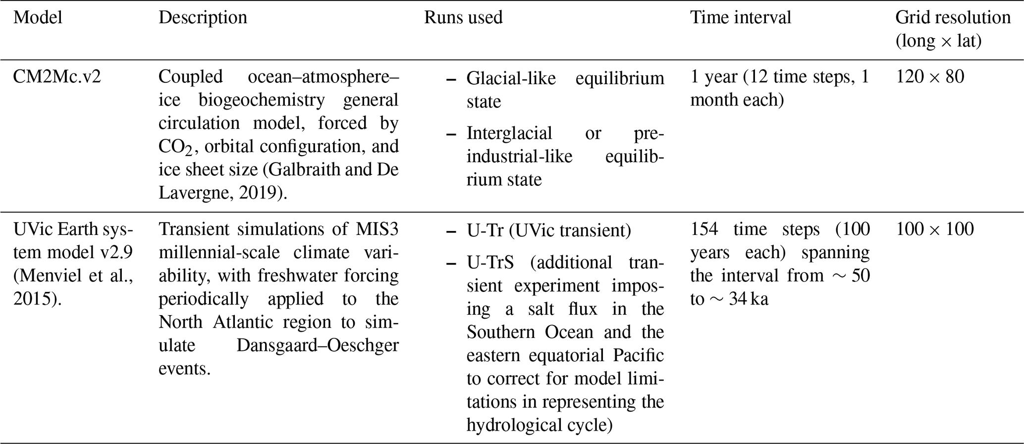
2.1 Model outputs

In order to explore regional associations in R-age variability, we make use of outputs from two different numerical models: CM2MC and UVic (Table 1). For the CM2Mc simulations, we use annual cycles drawn from an equilibrium interglacial-like state and from an equilibrium glacial-like state (Galbraith and De Lavergne, 2019). The UVic outputs consist of annual averages (at 100-year resolution) from two sets of transient simulations performed under “mid-glacial” boundary conditions equivalent to Marine Isotope Stage (MIS) 3 (Menviel et al., 2015). One of these simulations (U-Tr) involved variable buoyancy forcing applied to the North Atlantic, resulting in changes in the strength of the Atlantic meridional overturning circulation (AMOC). A second set of UVic simulations (U-TrS) also involved variable buoyancy forcing applied to the Indian and Pacific sectors of the Southern Ocean, as well as the eastern equatorial Pacific (EEP), resulting in additional changes in the strength of deep convection near Antarctica and in the northern Pacific (Menviel et al., 2015). The UVic simulations consist of two consecutive runs for each of the U-Tr and U-TrS simulations. The start of the second run was initialized far from equilibrium for radiocarbon and therefore includes a global spike in marine radiocarbon activity. This has been retained in our analyses to permit an assessment of our ability to identify regional clusters both with and without the occurrence of a large background global anomaly, such as would be produced by the a large geomagnetic excursion (Heaton et al., 2021).

The dissolved inorganic carbon (DIC) and the dissolved inorganic radiocarbon (DI¹⁴C) are used to compute surface ocean Δ¹⁴C:

$$\begin{array}{}\text{(5)}& \mathrm{\Delta }{}^{\mathrm{14}}\mathrm{C}=\left({\displaystyle \frac{{\mathrm{DI}}^{\mathrm{14}}\mathrm{C}}{\text{DIC}}}-\mathrm{1}\right)\times \mathrm{1000}.\end{array}$$

R-age offsets are then calculated, taking into account the atmospheric Δ¹⁴C_atm:

$$\begin{array}{}\text{(6)}& R_{\mathrm{age}}=-\mathrm{8267}\times \ln \left[\left({\displaystyle \frac{\mathrm{\Delta }{}^{\mathrm{14}}{\mathrm{C}}_{\mathrm{ocean}}}{\mathrm{1000}}}+\mathrm{1}\right)/\left({\displaystyle \frac{\mathrm{\Delta }{}^{\mathrm{14}}{\mathrm{C}}_{\mathrm{atm}}}{\mathrm{1000}}}+\mathrm{1}\right)\right].\end{array}$$

Here we use the “true” mean lifetime of radiocarbon (8267 years) based on the “Cambridge half-life” of 5730 years (Godwin, 1962). However, we note that if a direct quantitative comparison with measurements was to be performed, then the conventional “Libby half-life” of 5648 years should be used instead. The atmospheric Δ¹⁴C in the CM2Mc runs is held constant at 0 ‰, while in the UVic runs it is held at 393 ‰.

2.2 Unsupervised machine learning

2.2.1 K-means

The k-means algorithm (see Ahmed et al., 2020, for a recent review) divides data into a number k of clusters, defining the partitions such that each data point is as close as possible to the mean of its assigned cluster. For our purposes, the R-age time series of each ocean location on the model grid constitutes one data point for k-means, letting us map out which grid points are assigned to which cluster. We feed no prior geographical information to the algorithm; therefore, regions delineated by the algorithm are based on the similarity of their R-age histories alone.

2.2.2 K-medoids

The k-medoids algorithm is similar to k-means, but instead of converging on abstract cluster centroids it identifies cluster medoids, i.e. actual data points that best represent each cluster. K-medoids is more robust to noise and outliers in the data (Arora et al., 2016); furthermore, working with concrete data points as cluster centres, we can pinpoint their locations on the model grid. In the implementation we used, k-medoids was slower than k-means, so although most of the results and discussion sections focus on k-medoids and hierarchical clustering, much of the exploratory analysis involved k-means.

2.2.3 Selecting k for k-means and k-medoids

The main drawback of both k-means and k-medoids is that they require a priori knowledge of the number of clusters, k, to divide data into. We employ four methods (Table 2) to evaluate clustering performance as a function of the number of clusters over the range $\mathrm{2}\le k\le \mathrm{10}$. The Caliński–Harabasz (CH) index and the silhouette score penalize different aspects of cluster shape: CH generally increases with k because it favours splitting the data into many small clusters to minimize intra-cluster distances; the silhouette score generally decreases with k because it favours a few large, well-separated clusters.

Table 2 Methods to pinpoint the optimal number of clusters.

2.2.4 Time series normalization and subclusters

We run k-means and k-medoids clustering on both unnormalized (“raw”) and normalized time series. In the first case, clustering captures differences in both the amplitudes and shapes of the time series. In the latter case, only shape information is considered.

Because clustering on normalized time series disregards amplitude information, we perform a first round of clustering using normalized data to identify time series that share the same patterns of variability, regardless of amplitude. A second round of clustering, using unnormalized data, is then performed on each of these “shape-based” clusters. This allows us to identify amplitude-based “subclusters” within the shape-based clusters. The “optimal” number of subclusters within each cluster is chosen at runtime using the elbow method (see Sect. 2.2, Table 2).

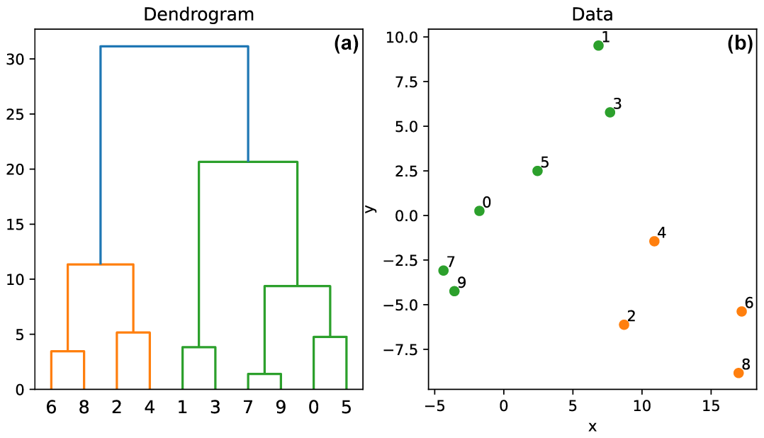
Figure 2 Illustration of the basic operation of the hierarchical clustering algorithm on synthetic data defined along two component axes. Note how points that plot closer together in panel (b) are recovered as more closely related in the dendrogram in panel (a).

2.2.5 Hierarchical clustering

Hierarchical clustering tells us how closely related data points are to each other, like phylogenetic trees. This requires the definition of an appropriate relatedness metric (or conversely, a distance metric). Using the Pearson correlation coefficient between the R-age histories of sites A and B in the ocean (ρ_AB), we may define a distance metric, $d=\sqrt{\mathrm{1}-{\mathit{\rho }}_{\mathrm{AB}}}$. This distance metric provides a measure of the similarity of two time series: d=0 when ρ_AB=1 (the distance between perfectly correlated time series is zero) and d=1 when ρ_AB=0 (uncorrelated time series are farther apart). The square root ensures that the triangle inequality is obeyed (Solo, 2019), avoiding misleading results (for example, when we fail to enforce the triangle inequality, we may obtain results where time series A is similar to B, B is similar to C, but A and C are dissimilar).

Given a matrix of distances between data points, there exist numerous methods to form a hierarchy or dendrogram (Fig. 2). We opt for the Ward method, which outperforms other common linkage methods where clusters overlap (Randriamihamison et al., 2019), as expected for our data. The resulting dendrogram illustrates cluster relatedness and has the advantage (over k-means and k-medoids) of not requiring prior information on the number of clusters. The dendrogram can be split (“flattened”) into an arbitrary number of clusters by cutting the tree at any height.

Figure 3 Clustering performance of k-means (left) and k-medoids (right) on unnormalized data as a function of the number of clusters over the range $\mathrm{2}\le K\le \mathrm{10}$ for the CM2Mc runs using unnormalized data (solid line for interglacial data, dotted line for glacial data). Vertical lines mark the elbow points. Note how for the interglacial case the elbow method and all three scores recover k=4 as a peak in clustering performance with k-means and k=6 with k-medoids.

2.2.6 Cluster analysis

The numerical cluster labels generated by the clustering algorithms are assigned randomly, hampering comparison between applications. To bypass this limitation, we (1) re-order cluster labels such that clusters with higher mean R ages are assigned smaller numbers and (2) define a re-labelling routine that takes in two sets of clustering results and attempts to permute the labels to maximize geographic overlap in cluster assignment between the two maps. Cluster maps with different grid sizes are re-gridded using a nearest-neighbour algorithm, and invalid data points (e.g. re-gridded onto land) are dropped from the analysis. As discussed below in Sect. 3, a one-to-one matching between the two sets of labels is not always possible.

Given a set of subclusters, we investigate to what extent the R-age time series belonging to each subcluster are described (1) by the subcluster medoid, (2) by the “parent” shape-based cluster medoid, and (3) by the running mean R age of the surface ocean. We take the difference between each of these three “benchmark” R-age time series and the subcluster member time series at each point in time, obtaining a distribution of R-age anomalies for each of the three cases. We compare the three anomaly distributions graphically as density plots and numerically in terms of their means.

Figure 4 Clustering results using k-medoids on unnormalized data from the CM2Mc interglacial run, using k=4.

3 Results

3.1 Equilibrium annual cycle for interglacial- and glacial-like states

Figure 3 summarizes the k-means and k-medoids clustering performance for different numbers of clusters (k), between k=2 and k=10. The clustering is applied to one annual cycle of unnormalized (raw) data from an interglacial-like climate state (solid lines in Fig. 3) and a glacial-like climate state (dashed lines in Fig. 3) simulated by the CM2Mc model (Galbraith and De Lavergne, 2019). Note that the Davies–Bouldin index has been multiplied by −1 to match the Caliński–Harabasz index and the silhouette score, such that lower values indicate diminishing explanatory power. For k-means, the four methods suggest k=4 as a particularly suitable number of clusters; it is pinpointed by the “elbow method” (vertical solid line, top-left panel) and rises above the background trends in the silhouette score, the CH index (slightly), and the DB index. A similar result is obtained for the glacial-like climate state using k-means (Fig. 3, left-hand plots, dashed lines). There is less agreement among the methods using k-medoids for the interglacial-like climate state (Fig. 3, right hand plots, solid lines), with an elbow apparent at k=4, peaks in silhouette scores, and the CH index and DB index at k=6. When applied to raw data from the glacial-like climate state, k-medoids also yield an elbow at k=4 and a strong peak in the CH index (Fig. 3 left-hand plots, dashed lines). Overall, for both k-means and k-medoids, no clear optimum value for k emerges for k>2 when using normalized data (Fig. 3), and this remains true when applied to normalized data (not shown).

In this context, where we are interested in the eventual construction of regional radiocarbon calibration curves, an optimal value of k will be the minimum value that provides a sufficient degree of explanatory power. Here, explanatory power reflects the degree to which the cluster centroid or medoid is able to represent the R-age history at a given location with sufficient accuracy and precision. Encouragingly, Fig. 3 suggests that for two very different equilibrium climate states the bulk of R-age variability can be captured with a relatively small number of clusters, e.g. k=4, and with little sensitivity to clustering method (e.g. k-means or k-medoids).

Figure 4 shows the clustering results for k-medoids applied to unnormalized CM2Mc interglacial data, using k=4. The cluster map in Fig. 4a illustrates the ocean regions corresponding to each cluster (landmasses in white), Fig. 4b shows all the R-age time series colour coded by cluster membership, and Fig. 4c shows time series associated with each cluster along with their respective centroids. Cluster no. 1 forms a longitudinal band in the Southern Ocean, featuring the highest mean R-ages and the strongest annual variation in R-age. Cluster nos. 2 and 3 cover a lower-latitude band within the Southern Ocean but also outcrop in the eastern equatorial Pacific (EEP) Ocean, the eastern central Atlantic Ocean, the North Atlantic Ocean, the northern Pacific Ocean, and the northern Indian Ocean. The rest of the ocean is assigned to cluster no. 4, which dominates the tropical and subtropical gyre regions and exhibits the lowest R-ages and least variability over the annual cycle. Increasing the number of clusters to k=9 further subdivides the ocean (Fig. S1) but with only a modest gain in explanatory power, producing the same broad patterns as for k=4.

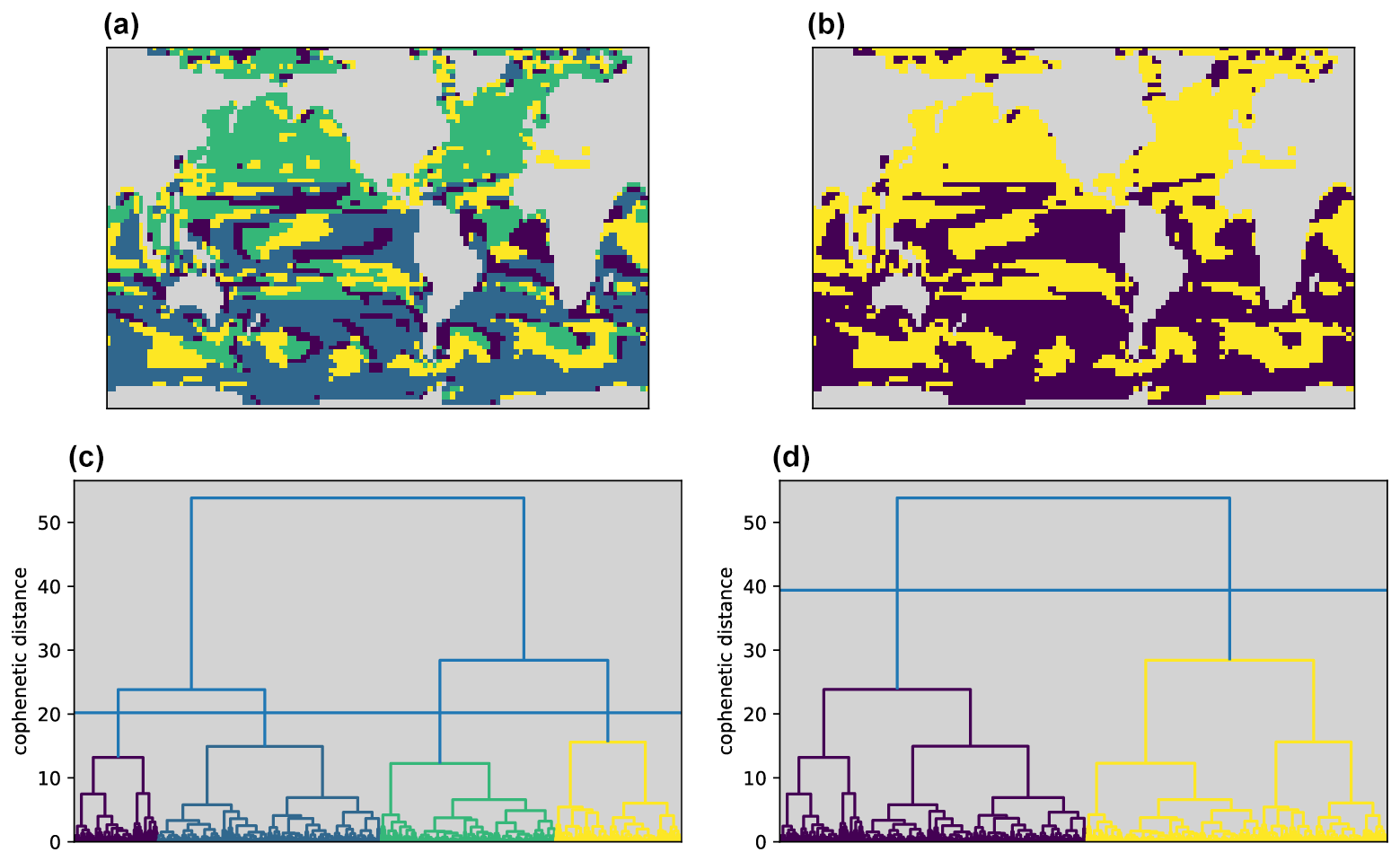
Figure 5 Hierarchical clustering results for the CM2Mc interglacial run based on Pearson distances between the R-age time series at each location. Panels (c) and (d) show the same cluster dendrogram but sliced at two different heights (cophenetic distances) to produce four and two clusters on the left and right, respectively. Panels (a) and (b) show the resulting cluster geographies, with landmasses in grey.

Clustering on normalized data to extract clusters based on time series shape alone (without amplitude information) produces highly geographically disconnected clusters for both k-means and k-medoids when k>2 (not shown). Nevertheless, a north–south divide is apparent in the clustering results for normalized data using k=4, reflecting an annual signal that is dominated by high-latitude seasonal convection and ocean–atmosphere gas exchange (also apparent in the centroid time series shown in Fig. 4c). The emergence of this north–south divide is further illustrated by hierarchical clustering on Pearson distances, which is also less sensitive to time series amplitude and recovers similar regions to the shape-based clustering (Fig. 5). The resulting dendrogram confirms that the north–south divide emerges at the highest branching level (Fig. 5, right panels).

Applying k-medoids to the glacial-like climate state simulated by CM2Mc, again using k=4, yields very similar (though not identical) results. This is shown in Fig. 6, which compares the clusters obtained for the glacial and interglacial states simulated using CM2Mc, demonstrating ∼ 80 % overlap. The similarity of the clusters obtained for the two simulations suggests minor differences in the overall impact of the annual cycle on the distribution of R-ages between two contrasting climate states. However, it is notable that the regions of non-overlap tend to occur at the margins of the clusters, suggesting an inherent ambiguity at the junctures of cluster regions (hatched areas in Fig. 6).

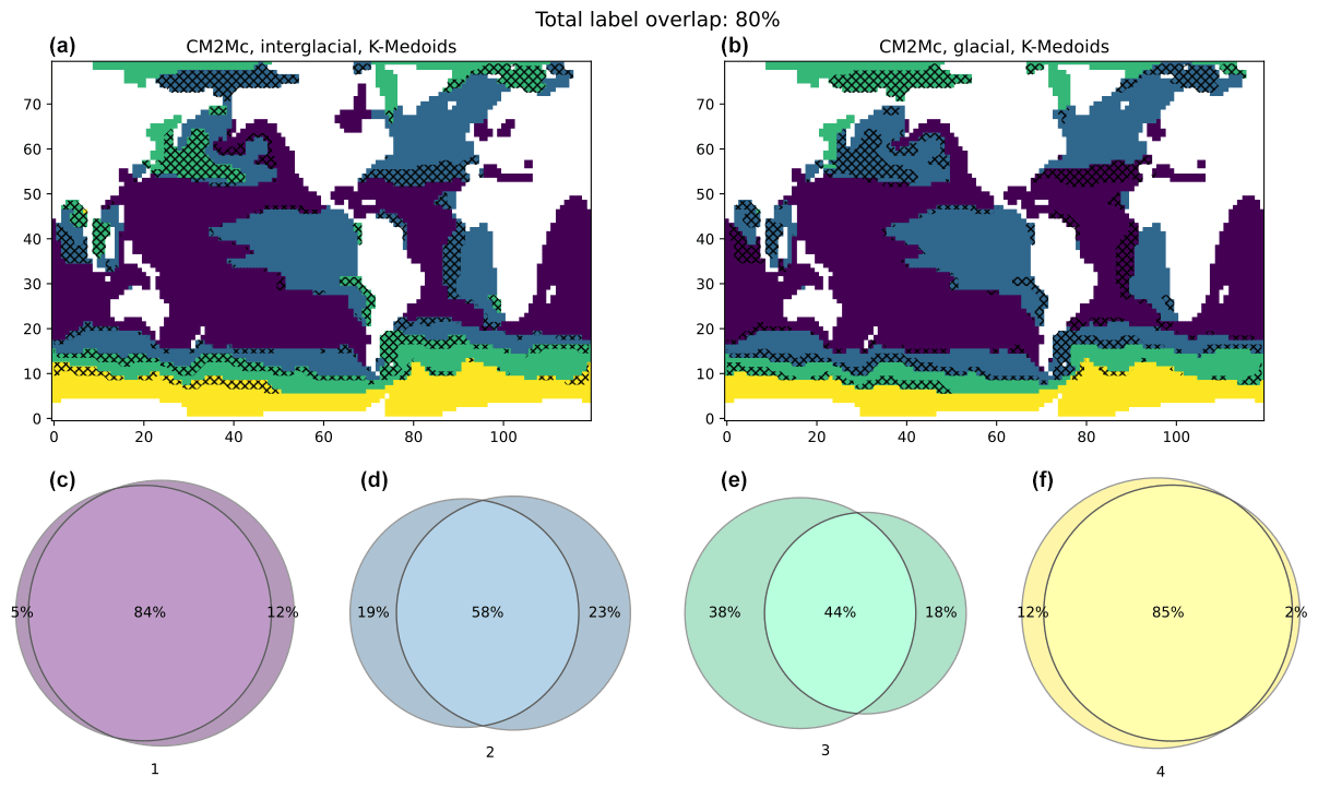
Figure 6 Comparison of clustering results between the two CM2Mc runs (a: interglacial; b: glacial) using k-medoids on unnormalized data. The colour-coded Venn diagrams quantify overlap between the two maps. For example, cluster no. 3 (green) is assigned substantially more area in the interglacial run on the left, while cluster no. 4 (yellow) covers roughly the same geographic region in both runs.

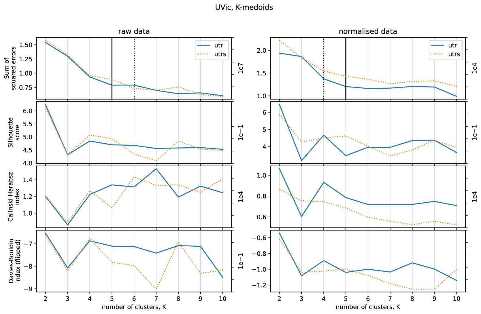
Figure 7 Clustering performance of k-medoids on unnormalized (left) and normalized (right) data as a function of the number of clusters over the range $\mathrm{2}\le K\le \mathrm{10}$ for the UVic runs (solid line: U-Tr data; dotted line: U-TrS data). Vertical lines mark the elbow points.

3.2 Transient freshwater hosing experiments

Figure 7 illustrates k-medoids clustering metrics for raw and normalized data (mean annual, in 100-year time steps) from the U-Tr and U-TrS simulations, which involved transient buoyancy forcing applied in the North Atlantic, as well as the Southern Ocean and EEP, against a mid-glacial background climate state equivalent to Marine Isotope Stage (MIS) 3 (Menviel et al., 2015) (see Table 1). Similar to the CM2Mc results, optimal values of k for the UVic outputs appear to lie at 4, 8, or 9. For comparison with the CM2Mc clustering results on unnormalized data, we choose to cluster the U-Tr and U-TrS data using k=4. The U-Tr clustering results using k-medoids on normalized data (k=4) are shown in Fig. 8. Broadly similar results are obtained when using k-means instead (not shown). The regional clusters that emerge from the U-Tr data broadly correspond to the major ocean basins (Fig. 8a). The Arctic Ocean (cluster no. 2) shows strong R-age variability, the Atlantic Ocean (no. 3) has smaller R-age peaks, the R-age time series of the Southern Ocean (no. 1) are rather flat compared to the others, and the Indo-Pacific cluster (no. 4) features broader and less accentuated maxima (Fig. 8c). Again, increasing the number of clusters to k=8 results in further splitting of the ocean basins (e.g. isolating the North Atlantic and the southern half of the Pacific) but with broadly the same basin-wide divisions as for k=4 (Fig. S2).

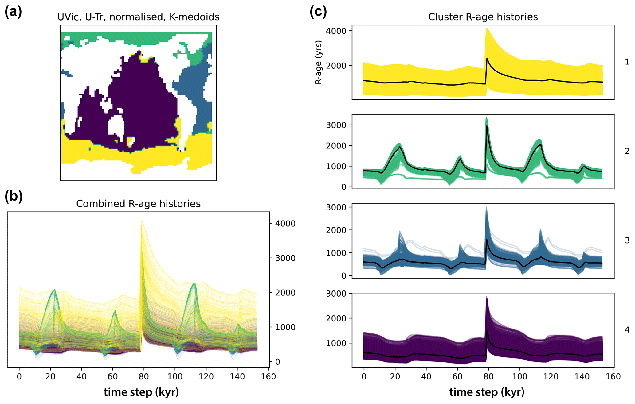
Figure 8 Clustering results using k-medoids on UVic (U-Tr run) normalized data. The layout is the same as for Fig. 4. Note how normalization produces clusters of similarly shaped R-age histories, regardless of their amplitudes.

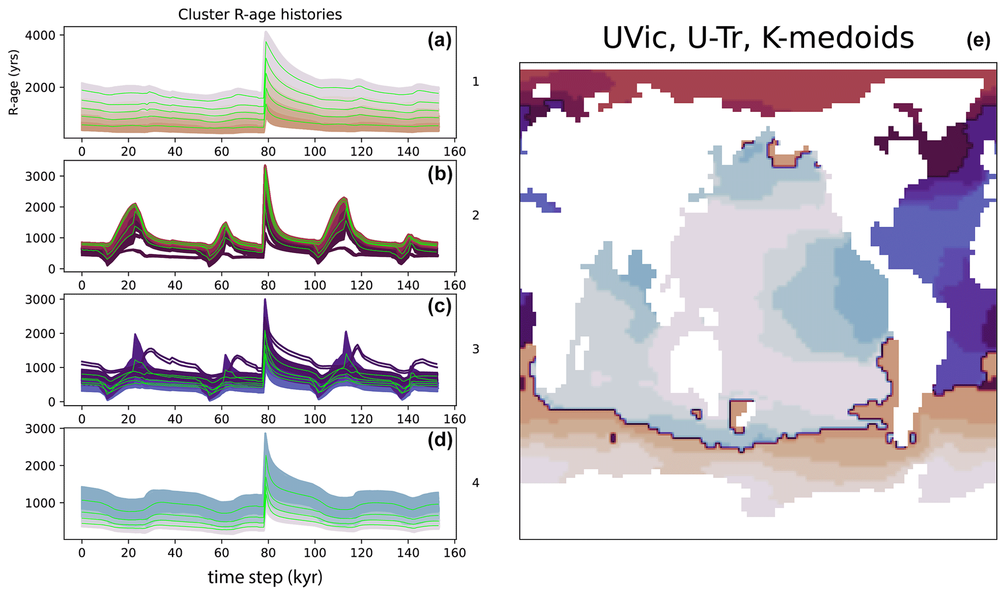
Figure 9 Clustering results using k-medoids on UVic (U-Tr run) data in two stages, whereby the shape-based clusters from Fig. 8 are further subdivided by re-applying k-medoids to unnormalized data. The left plot shows R-age time series grouped by cluster nos. 1–4, with sub-clusters identified by shading and sub-cluster medoids shown by heavy green lines. (e) Map of R-age clusters (identified by colours) and sub-clusters (identified by shades of each colour). Note how the subclusters are distinguished by their mean R-ages.

To explore the possibility of identifying sub-regions of similar amplitude variability, within each shape-based cluster, we perform a second round of clustering on unnormalized data from within each of the four shape-based clusters shown in Fig. 8. The results are shown in Fig. 9, demonstrating a decrease in the amplitude of R-age variability with decreasing latitude in the Southern Ocean, the Arctic Ocean, and the North Atlantic, despite distinct patterns of variability in each of these regions. Similarly, there is a decrease in R-age amplitude away from some ocean margins, e.g. in the EEP Ocean, the eastern central Atlantic Ocean, the northern Pacific Ocean, and the northern Indian Ocean.

Like with the CM2Mc data, hierarchical clustering of the U-Tr data based on Pearson correlations (Fig. 10, left side) produces similar geographic patterns to k-medoids clustering on normalized data. The Arctic Ocean is most closely related to the North Atlantic on the dendrogram. Meanwhile, the central Atlantic is more related to the Southern Ocean than to the North Atlantic, marking a north–south divide high up on the dendrogram highlighted in Fig. 10 (right side). The northern Pacific stands out from the rest of the Pacific, but overall the Pacific appears to be more closely related to the central Atlantic and Southern Ocean than to the Arctic and North Atlantic.

Figure 10 Hierarchical clustering results for the UVic U-Tr run. Panels (c) and (d) show the same cluster dendrogram but sliced at two different heights (cophenetic distances) to produce seven and two clusters on the left and right, respectively. Panels (a) and (b) show the resulting cluster geographies, with landmasses in grey.

Figure 11 Comparison of clustering results between the UVic U-Tr run (a) and the CM2Mc glacial run (b) using k-medoids on unnormalized data. The colour-coded Venn diagrams quantify overlap between the two maps. Part of the mismatch is attributable to differences in coastal boundaries and model resolutions (here UVic results are re-gridded to permit comparison to CM2Mc).

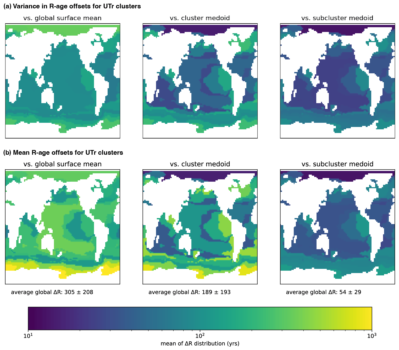
Figure 12 The variance (a) and mean (b) of the distribution of R-age offsets in the UVic U-Tr data when computed relative to three different references: the running mean of the global surface ocean, analogous to, e.g. Marine20 (column 1); the medoid of the shape-based cluster to which the subcluster belongs (column 2); and the subcluster's own medoid (column 3). The decreasing magnitudes from left to right suggest an increase in the accuracy with which the calibration captures R-age histories in each subcluster, with sub-cluster medoids providing the greatest accuracy. This suggests that regional calibrations, e.g. for cluster or sub-cluster regions, could provide more accurate calibrations than constant delta-R values applied to a global mean estimate such as Marine20.

A comparison of results obtained for normalized data from U-Tr (North Atlantic hosing) and U-TrS (North Atlantic hosing with Southern Ocean buoyancy forcing) indicates cluster overlap ∼95 % (Fig. S3), with differences primarily occurring along the northern margin of the Southern Ocean. The difference between the two UVic simulations is smaller than the difference between the two CM2Mc simulations. Most significantly, a comparison of clusters obtained using k-medoids applied to unnormalized data from the U-Tr simulation (transient annual averages) and the glacial CM2Mc simulation (equilibrium annual cycle) yields an overlap of ∼70 % (Fig. 11). Here the main difference arises from the identification of a region of distinct annual variability in the sub-polar Southern Ocean in the glacial CM2Mc simulation, which is not present in the transient U-Tr simulation. Overall, the regional clusters that are obtained in the three different sets of model runs exhibit a good degree of coherence, and it is particularly encouraging that similar regional clusters are obtained for model runs with completely different boundary conditions and timescales of variability (Fig. 11). This would suggest that the regional clustering of R-age variability may be broadly independent of how and why R-ages have changed, and therefore the regional clusters would apply to a wide range of possible R-age scenarios (including those realized in the past).

4 Discussion

The broad similarity of the clustering results obtained across the suite of equilibrium and transient simulations (Figs. 6, 11 and S3) suggests that the regional R-age associations arise to a large extent from fundamental aspects of global ocean and climate dynamics. For example, the hemispheric partitioning in normalized annual cycle data from both glacial and interglacial climate states clearly reflects the dominant influence of the annual cycle. Similarly, the regional clusters obtained in unnormalized annual cycle data (Fig. 4) and especially in transient annual average data (Fig. 8) appear to reflect provinces of distinct hydrographic variability that are defined by fundamental oceanographic characteristics such as the presence, absence, and variability of sea ice, deep mixing, or upwelling. Such features are typically geographically “locked”, despite being varying in time in their intensity and expression. It was an appreciation of such regional specificity in the mechanisms that control R-age variability that provided an initial justification for using constant corrections to the global mean R-age (i.e. delta-R values) as an approximation of past local R-age variability (Stuiver et al., 1986). R-ages in regions with extensive sea ice cover, deep mixing, or upwelling will always be offset to higher values as compared to the global mean. In the U-Tr and U-TrS simulations, the Arctic and Antarctic R-age clusters broadly coincide with regions of similarly coherent sea ice variability (not shown), though the overlap is not perfect, suggesting that a more complex array of processes controls the regionalism in R-age variability. The clustering results for the CM2M2 simulations suggest that regional seasonality (in sea ice, mixed-layer depth, etc.) may play a contributing role. Here, our primary interest is in the viability of the clustering approach when applied to realistic (i.e. modelled) R-age variability, rather than the precise reasons for the variability itself. Nevertheless, some regional associations appear not to have any plausible physical link at all, e.g. the grouping of the Arctic and sub-Antarctic in Fig. 4. Although the regional calibration curves for these two regions might look very similar, it seems sensible to suggest that any given regional calibration curve should probably only be applied to a single geographically contiguous area. In any event, a detailed analysis of the controls on regional R-age variability in model simulations that aim specifically to reproduce R-age reconstructions represents an important target for future work, which we do not address in this study. Here clustering may also yield useful insights.

In addition to stable “regionality” of R-age behaviour, the use of delta-R values over long spans of time further requires that regional R-ages follow the same temporal trends as the global mean. As noted when the delta-R approach to marine radiocarbon calibration was formulated (Stuiver et al., 1986) and as illustrated by the U-Tr and U-TrS simulations (e.g. Figs. 8 and 9), such global coherence cannot necessarily be expected when the ocean–climate system undergoes significant change (see also Fig. 1b). Changes in sea ice cover, mixed-layer depth, upwelling strength, etc., will change the difference between a local R-age and the global mean (i.e. delta-R). Therefore, a key question for radiocarbon calibration is whether regional clusters (and sub-clusters) as identified here can provide more accurate estimates of past R-age variability at a given location than is provided by, e.g. the global mean (± a constant correction, delta-R).

Figure 13 Tentative hierarchical clustering of available R-age reconstructions spanning the last deglaciation (Skinner et al., 2023) compared with grouping of proxy observations according to location and corresponding model-based clusters. (a) R-age time series locations and proxy-based cluster membership (coloured circles) superposed on a map of model-derived shape-based hierarchical clusters (numbered 1 to 4) for the U-TrS simulation: filled green circles indicate proxy observation cluster 1; filled blue circles indicate proxy observation cluster 2; and red and blue outlines indicate low- and high-amplitude sub-cluster membership, respectively. Two clusters and sub-clusters were employed for the proxy-based clustering due to the sparsity of available time series. (b–e) Greenland NGRIP and Antarctic EPICA Dome C (EDC) ice core temperature proxy records (the heavy black line is the three-point running mean) compared with R-age data grouped according to model-based clusters (four shape-based clusters and two amplitude-based sub-clusters). Dashed lines indicate R-age data (binned and interpolated; see text), and thick solid lines indicate means of the time series that belong to each model-based sub-cluster. Direct clustering of the proxy observations is shown to be broadly consistent with the model-based clustering.

Here, this question can be answered for the model outputs by comparing the magnitude, and in particular the variance, of offsets between local R-ages and (1) the global mean R-age, (2) the associated (shape-based) cluster centroid, and (3) the (amplitude-based) sub-cluster centroid. The variance in these offsets is important because it reflects the degree to which a constant correction, e.g. applied to a global average calibration curve (a delta-R value), would be wrong on average. Figure 12 illustrates the spatial distributions for each of these offsets and their variance based on the U-Tr outputs. In Fig. 12, the largest R-age offsets and the greatest variance in R-age offsets occur when referencing to the global mean surface R-age (305±208 ¹⁴Cyrs). The smallest magnitude and variance occur when referencing to the centroid of the relevant amplitude-based sub-cluster (54±29 ¹⁴Cyrs), and an intermediate gain in accuracy is achieved when referencing to the centroid of the wider shape-based cluster (189±93 ¹⁴Cyrs). Encouragingly, a similar stepwise improvement in accuracy is found when shape-based clusters or amplitude-based sub-clusters from the U-Tr simulation are used to assess R-age offsets in the glacial CM2Mc simulation (e.g. average offsets of 259±227 ¹⁴Cyrs for the global mean versus 79±36 ¹⁴Cyrs for sub-cluster centroids; Fig. S4).

The above discussion would suggest that radiocarbon calibrations performed using a regional calibration curve, particularly one derived at an appropriate sub-cluster centroid location, could be more accurate than calibrations performed using a global mean calibration curve in conjunction with a constant delta-R value. By way of illustration, an R-age (or delta-R) uncertainty of 200 (versus 30) ¹⁴C yrs would result in a calibrated age uncertainty of ∼540 (versus ∼170) when calibrating a radiocarbon date of 20 000±150 ¹⁴C years. Similarly, a delta-R error or bias of up to ∼1000 ¹⁴C years, as is observed at high southern latitudes in the UVic simulations (Fig. 1b), would result in a calibrated age error or bias of ∼1000 years. Notably, the above analysis likely underestimates the uncertainty associated with using a global mean calibration curve and constant delta-R value in practice, since it assumes perfect knowledge of the evolving global mean R-age (i.e. a global mean radiocarbon calibration). As noted above, our best estimate of the mean ocean R-age history is currently based on modelling and therefore assumptions regarding past ocean circulation and climate change (Heaton et al., 2020).

While our analysis provides an illustration of the viability and the utility of defining regions for which local calibrations might be constructed, it only does so theoretically using model outputs. However, the fact that regional clusters can successfully be identified in model outputs is in itself consistent with the observation of distinct regional patterns in R-age reconstructions, e.g. from the northeastern Atlantic, Iberian Margin, South Atlantic, and Southern Ocean (Skinner et al., 2019). The further observation of similar but lower-amplitude R-age trends on the Iberian Margin versus the northern northeastern Atlantic and in the South Atlantic versus the Southern Ocean also resonates with the sub-cluster results obtained from the U-Tr and U-TrS outputs, as does the observation of an apparent link between the high southern latitudes and the eastern equatorial Pacific (De La Fuente et al., 2015) (Fig. 11).

The regional patterns picked out by clustering of model outputs are further confirmed by a tentative hierarchical clustering performed on 23 available shallow sub-surface R-age reconstructions from <500 m water depth (or <1000 m in the Southern Ocean). For this analysis, time series were selected that include at least six data points from the 5–21 ka BP interval, which were binned and interpolated onto 500-year intervals. Using normalized data and k=2 (given the lack of data from, e.g. the Arctic, Indian, or northern Pacific oceans), hierarchical clustering of the proxy data identifies a dominant signal in the North Atlantic (Fig. 13, blue circles) that is distinct from the primary signal observed in the Southern Ocean and Pacific Ocean (Fig. 13, green circles). Amplitude-based sub-clusters from within these regional shape-based clusters (again with k=2) generally also manage to isolate higher-amplitude, high-latitude, and eastern equatorial upwelling signals (Fig. 13, blue-outlined circles) from lower-amplitude low-latitude signals (Fig. 13, red-outlined circles). These proxy observation-based clusters (Fig. 13b–e) are generally consistent with the model-based hierarchical clusters (U-TrS, four clusters, and two sub-clusters) that correspond to the proxy time series locations (filled circles in Fig. 13a).

Thus, the model-based clustering correctly predicts higher-amplitude signals in the eastern equatorial upwelling region, the Southern Ocean, and the high-latitude North Atlantic. Furthermore, when grouping the R-age data using either direct hierarchical clustering or model-based cluster membership, the dominant signals that emerge appear to track Greenland and Antarctic temperature variability, as observed for example by Skinner et al. (2019). Although the similarities between proxy observation- and model-based regional clustering are encouraging, it should be noted that the clustering of proxy data is not especially robust and is highly sensitive to data selection and parameter selection (e.g. k, minimum time series length). A far larger number of better-resolved surface reservoir age data, spanning a greater geographical range, will be needed to improve upon the highly tentative data-based regional clusters shown in Fig. 13. Nevertheless, the results are encouraging and suggest that the generation of regional marine radiocarbon calibration curves for the high-latitude and mid-latitude northeastern Atlantic (i.e. Iberian Margin) is already a viable prospect.

5 Conclusions

K-means, k-medoids, and hierarchical clustering reveal distinct regions of coherent R-age behaviour in the surface ocean, subject to a range of perturbations, from seasonal to millennial timescales. In this context, the optimal value of k (the number of clusters) is difficult to define robustly a priori and appears to depend on the method and the input data selected. The regional clusters that are obtained, across the range of modelled oceanographic perturbations investigated, tend to cohere in a broadly consistent manner with specific geographic domains, which in turn appear to reflect fundamental oceanographic and/or seasonal controls on relevant processes such as sea ice variability, upwelling, and mass divergence. Clustering thus confirms geographic controls on the variability in R-ages and their offset from the global mean surface ocean R-age (Stuiver et al., 1986). At larger spatial scales, clustering reveals broadly basin-scale associations in the “character” (shape) of R-age variability. These large-scale shape-based clusters may be further sub-divided into regional amplitude-based sub-clusters. Comparisons within and between different model simulations, different timescales, and different models indicate that calibration curves constructed at appropriate locations, representative of the regional sub-cluster medoids or centroids, would yield significantly more accurate calibrated radiocarbon dates than provided by the standard approach that assumes constant delta-R values. Furthermore, a tentative application of these methods to existing R-age data identifies similar regional associations as compared to the numerical model outputs. Substantially more and better-resolved R-age reconstructions covering more of the worlds' ocean basins will be needed before robust regional radiocarbon calibrations can be fully tested and applied. Nevertheless, based on our results, machine learning appears to be a promising approach to the problem of defining regional marine radiocarbon calibration curves. The generation of such observation-based regional calibration curves (along with well-defined regions of applicability) would represent an alternative and complementary approach to that already proposed for marine radiocarbon age calibration at high latitudes based on forward modelling (Alves et al., 2019; Heaton et al., 2023). One advantage of the approach advocated here is that it does not require explicit modelling of past R-age variability and therefore does not assume a priori knowledge of past ocean circulation, sea ice, carbon cycling, etc. While the paucity of existing R-age reconstructions currently restricts our ability to deploy regional marine radiocarbon calibrations across the globe, the mid- and high-latitude sectors of the northeastern Atlantic emerge as the most promising regions for initial progress in this regard.