The quantification of down-hole fractionation for laser ablation mass spectrometry

Down-hole fractionation (DHF), a known phenomenon in static spot laser ablation, remains one of the most significant sources of uncertainty for laser-based geochronology. A given DHF pattern is unique to a set of conditions, including material, inter-element analyte pair, laser conditions, and spot geometry. Current modelling methods (simple or multiple linear regression, spline-based regression) for DHF do not readily lend themselves to uncertainty propagation, nor do they allow for quantitative inter-session comparison, let alone inter-laboratory or inter-material comparison.

In this study, we investigate the application of orthogonal polynomial decomposition for quantitative modelling of LA-ICP-MS DHF patterns. We outline the algorithm used to compute the models, apply it to an exemplar U–Pb dataset across a range of materials and analytical sessions, and finally provide a brief interpretation of the resulting data.

In this contribution we demonstrate the feasibility of quantitative modelling and comparison of DHF patterns from multiple materials across multiple sessions. We utilise a relatively new data visualisation method, uniform manifold approximation and projection (UMAP), to help visualise the data relationships in this large dataset while comparing it to more traditional methods of data visualisation.

The algorithm presented in this research advances our capability to accurately model LA-ICP-MS DHF and may facilitate reliable decoupling of the DHF correction for non-matrix-matched materials, lead to improved uncertainty propagation, and facilitate inter-laboratory comparison studies of DHF patterns.

The generalised nature of the algorithm means it is applicable not only to geochronology but also more broadly within the geosciences where predictable linear (x-to-y) relationships exist.

1 Introduction

LA-ICP-MS of geological materials has significantly advanced since its adoption at the end of the 20th century and is today the technique of choice for most applications for mineral geochronology. Initial geochronological studies on zircon were only able to produce tens of individual data per session due to technical, time, and computing limitations (e.g. Hirata and Nesbitt, 1995). Nowadays high-precision individual analyses on multiple minerals using a range of geochronologic systems (e.g. U–Pb, Rb–Sr, Lu–Hf, Re–Os) can be rapidly and accurately acquired (Chew et al., 2019; Gehrels et al., 2008; Glorie et al., 2023; Hogmalm et al., 2017; Kendall-Langley et al., 2020; Larson et al., 2024; McFarlane, 2016; Mohammadi et al., 2024; Roberts et al., 2020; Simpson et al., 2021; Subarkah et al., 2021; Tamblyn et al., 2024; Zack et al., 2011). However, to achieve accurate, high-quality data, correction procedures need to be implemented, including calibration to reference material(s) (RM), corrections for matrix offsets, and inter-element down-hole fractionation (DHF) (Agatemor and Beauchemin, 2011; Allen and Campbell, 2012; Gilbert et al., 2017; Günther et al., 2001; McLean et al., 2016; Ver Hoeve et al., 2018). As DHF is a geometry-dependent spot-ablation phenomenon unique to each material and (inter-element) analyte ratio pair (e.g. NIST SRM glasses, zircon, ${}^{\mathrm{206}}\mathrm{Pb}{/}^{\mathrm{238}}\mathrm{U}$, ${}^{\mathrm{207}}\mathrm{Pb}{/}^{\mathrm{235}}\mathrm{U}$, ${}^{\mathrm{87}}\mathrm{Rb}{/}^{\mathrm{87}}\mathrm{Sr}$), it cannot be corrected via ICP-MS tuning (Mank and Mason, 1999). However, DHF can be optimised to balance the overall count rate against the magnitude of DHF by adjusting the spot geometry and fluence parameters for analysis of a given material (Guillong and Günther, 2002; Košler et al., 2005). Researchers have proposed several methods for minimising DHF, typically by surface rastering or limiting acquisition times to short intervals; however, these compromise either the spatial or temporal resolution of analysis (Horstwood et al., 2003; Paton et al., 2010). Alternatively, regression modelling can be used to correct DHF during the data reduction process either using a predetermined empirical model or fitting a model to the observed data (e.g. Horn et al., 2000; Paton et al., 2010). Currently, the latter method of fitting a regression model to the observed DHF pattern of an RM then applying that model to unknowns is used by commercial data reduction software (e.g. LADR: Norris and Danyushevsky, 2018; Iolite: Paton et al., 2011) for DHF correction in LA-ICP-MS methodology. In this process a matrix-matched RM is used (or a glass RM if no suitable matrix-matched material is available) and requires the assumption that the unknowns (i.e. target samples) have the same DHF behaviour as the RM. If the modelled RM poorly matches the DHF of the unknown, it will introduce some artefact (user-induced error) that may either increase the uncertainty of the observed ratio of the unknowns if using a time-matched signal or result in over- or underestimation of the observed ratio if using a subset of the signal (Fig. 1).

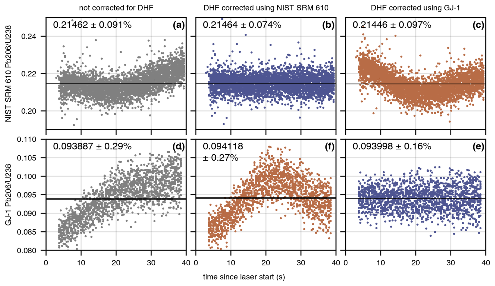
Figure 1 Demonstration of the impact of using an inappropriate material to correct down-hole fractionation (DHF). The two rows are ${}^{\mathrm{206}}\mathrm{Pb}{/}^{\mathrm{238}}\mathrm{U}$ ratios for NIST SRM 610 glass (a–c) and GJ-1 zircon (d–f), collected in a single session. The columns from left to right are not corrected for DHF (grey points, raw ratios), DHF corrected using NIST SRM 610 as the model, and DHF corrected using GJ-1 as the model. Blue points indicate an appropriate DHF correction (e.g. GJ-1 by GJ-1), while orange points indicate an inappropriate DHF correction (e.g. GJ-1 by NIST SRM 610). Black horizontal spans indicate the geometric mean and its asymmetric lower and upper 2 standard error for each data set. The percent error shown is 2 standard error level of the larger geometric standard error (usually upper uncertainty). Note the significantly larger error for the inappropriate corrections (orange points) compared to the appropriate (blue) corrections. These uncertainties would then propagate into further processing steps to obtain accurate LA-ICP-MS ratios (e.g. calibration to a known value).

Additionally, these modelling methods (i) do not readily lend themselves to arithmetic propagation of their uncertainties (Paton et al., 2010), (ii) require an arbitrary user choice for the fitting method (simple or multiple linear regression polynomial order, or non-linear regression), and (iii) cannot be quantitatively compared between laboratories or even intra-laboratory analytical sessions. Thus, inter-element DHF remains one of the largest sources of uncertainty for LA-ICP-MS analyses and is difficult to either qualitatively or quantitatively compare (Horstwood et al., 2016).

Here we present a technique to numerically quantify processes in the geosciences which can be modelled by a linear combination of basis functions (e.g. DHF) using the coefficients of orthogonal polynomials fit to the signals. We develop upon the algorithms for quantitative modelling of rare earth element patterns by O'Neill (2016) and Anenburg and Williams (2022). Our modified implementation of these algorithms uses input uncertainties as weights and can be more generally applied to data where there is a predictable x-to-y relationship. Here we demonstrate the technique's application for modelling DHF in a quantitative manner.

Using a LA-ICP-MS dataset (time, ratio of analytes), an orthogonal decomposition is used to fit a polynomial to the signal data by generalised least squares (Fig. 2). This method of using orthogonal polynomial decomposition during model fitting enables the quantitative comparison of DHF patterns via their coefficients for data from different analyte ratio pairs, for varied materials, and for inter-session (Fig. 2) and inter-laboratory datasets. Furthermore, this fitting method allows for improved computation of the uncertainty for each coefficient (and thus overall fit) and their covariances which can then be propagated into the final result.

In this research we highlight the utility of the algorithm for numeric comparison of the U–Pb DHF patterns from a range of natural and synthetic RMs used for U–Pb age date calibration. We envisage that this algorithm could be used to self-correct individual analyses for DHF (or as spline bases for signals that display zonation, e.g. different age domains), with a fall back to a known RM in the case of particularly noisy (analytical noise) data. This would allow reliable decoupling of the DHF correction for non-matrix-matched materials and propagation of the uncertainty in the down-hole model into the result, thereby improving the accuracy and precision of LA-ICP-MS analyses.

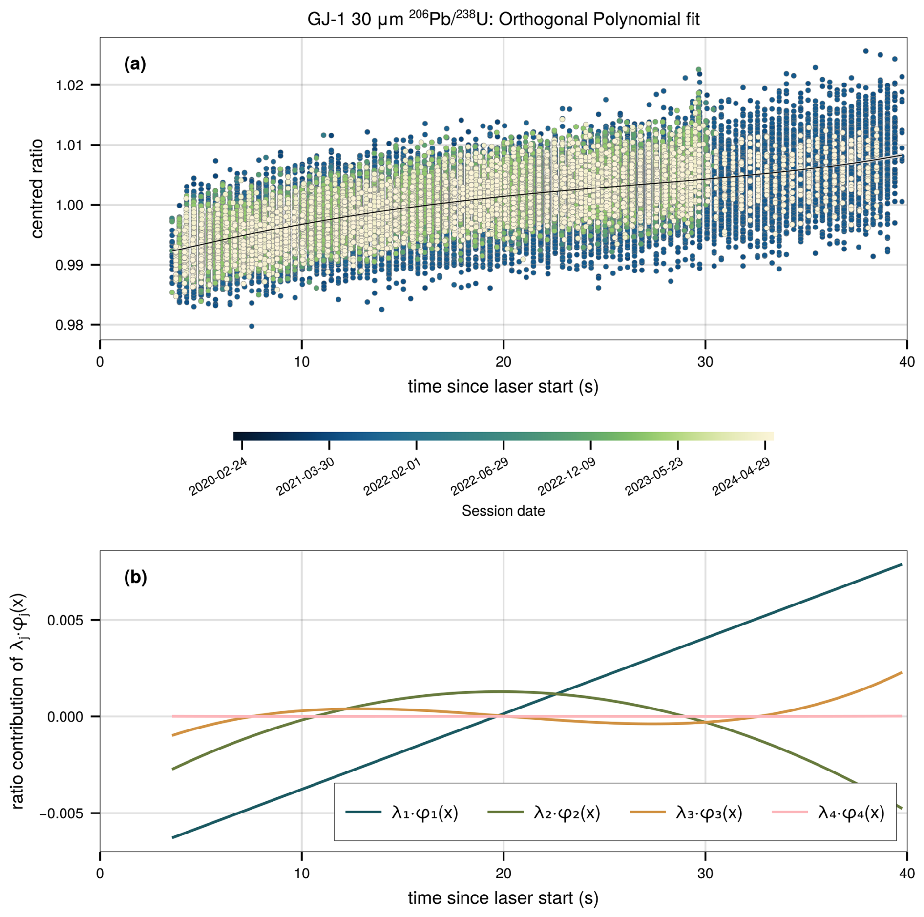
Figure 2 (a) Centred, point-wise ${}^{\mathrm{206}}\mathrm{Pb}{/}^{\mathrm{238}}\mathrm{U}$ ratios for all zircon GJ-1 analyses measured in multiple analytical sessions from 2020 to 2024 that used the same laser parameters. All analyses in this subset of data were collected using a 30 µm spot diameter, 5 Hz repetition rate, and nominal fluence of 2.0 J cm⁻². The black line is the fitted orthogonal polynomial, with grey shading indicating the 95 % confidence interval of the fit. The shaded confidence interval is barely visible due to its small absolute range. (b) Individual orthogonal components (i.e. the result of λ_j⋅φ_j(x)) of the fit in the upper panel excluding λ₀ (mean ratio, i.e. vertical central tendency) as this is a function of mass-spectrometer tuning and not a result of down-hole fractionation (DHF). φ_j is the orthogonal function evaluated at x^j (i.e. $x^{\mathrm{0}},x^{\mathrm{1}},x^{\mathrm{2}},\mathrm{\dots }$) for j=1 to order k. For this aggregated GJ-1 data, different mass-spectrometer tuning parameters and drift are accounted for by centring the data (subtraction of geometric mean and adding a constant of 1) resulting in λ₀≈1. Components λ₁ and higher represent the increasing shape component (linear slope, quadratic curvature, etc.) of the observed DHF pattern. Note in this case the magnitude of λ₄ is approximately zero, and as such, the result of λ₄ is approximately a horizontal line at zero. The sum of all components forms the polynomial in the upper panel.

2 Experiment

To improve our ability to assess, quantify, and compare DHF we implement a method of orthogonal polynomial decomposition to perform multiple linear regression (polynomial) model fitting to time-resolved analytical data from ICP-MS instruments. In keeping with the terminology of O'Neill (2016) and Anenburg and Williams (2022) we use the term lambda (λ) coefficients to denote the polynomial coefficients derived from models using orthogonal decomposition.

Unlike regular linear regression fitting, the implementation of orthogonal polynomial decomposition for regression modelling imparts the property of independence on lower-order polynomial coefficients from their higher-order counterparts (Bevington and Robinson, 2003). That is to say that the first coefficient is independent of the second- and higher-order coefficients, while the second coefficient is independent of the third- and higher-order coefficients and so forth. In practice, this means that the values of the polynomial coefficients are stable (you can fit a first- or second-order polynomial to some data and the value of first coefficient will not change) and they have some physical meaning in relation to the data. In the case of DHF data, λ₀ (the first coefficient) represents the (arithmetic) mean ratio, while λ₁ and higher are the shape parameters that represent the DHF pattern (Fig. 2). For example, λ₁ represents the linear slope (mean rate of change in ratio), while λ₂ represents the quadratic curve of the DHF pattern (Fig. 2). The independence and physical meaning of the lambda coefficients allows them to be used to quantitatively compare independent fits (e.g. single analyses, materials, analytical sessions, differing laboratories) so long as other parameters (e.g. fluence, spot diameter/volume, laser wavelength) are considered. Further details on the fitting algorithm and mathematics behind this process are outlined below in Sect. 2.2, detailed in Appendix A, and described in Bevington and Robinson (2003), O'Neill (2016), and Anenburg and Williams (2022). The raw data ingestion and required preprocessing steps are outlined below in Sect. 2.1.

Code written to perform the data ingestion, preprocessing, and fitting was written in the Julia (version 1.10, LTS) programming language (Bezanson et al., 2017). The code forms part of an in-development Julia package, GeochemistryTools.jl, that will be formally released in the future. Should users want early access to the package or source code for the algorithms outlined in this paper, they are available via GitHub (see “Code and data availability”). Figures were generated using the Makie.jl plotting library (Danisch and Krumbiegel, 2021) using “Scientific colour maps” (Crameri et al., 2020) implemented in ColorSchemes.jl.

2.1 Data ingestion and preprocessing

Data were imported from the raw ICP-MS CSV files; in this case from Agilent ICP-MS instruments. The algorithm written for this task processes the individual files (which can be a single analysis, a specified sample, or entire session) and performs several operations, outlined in Fig. 3, on user-specified mass counts-per-second (CPS) columns (i.e. channels, analyte signals).

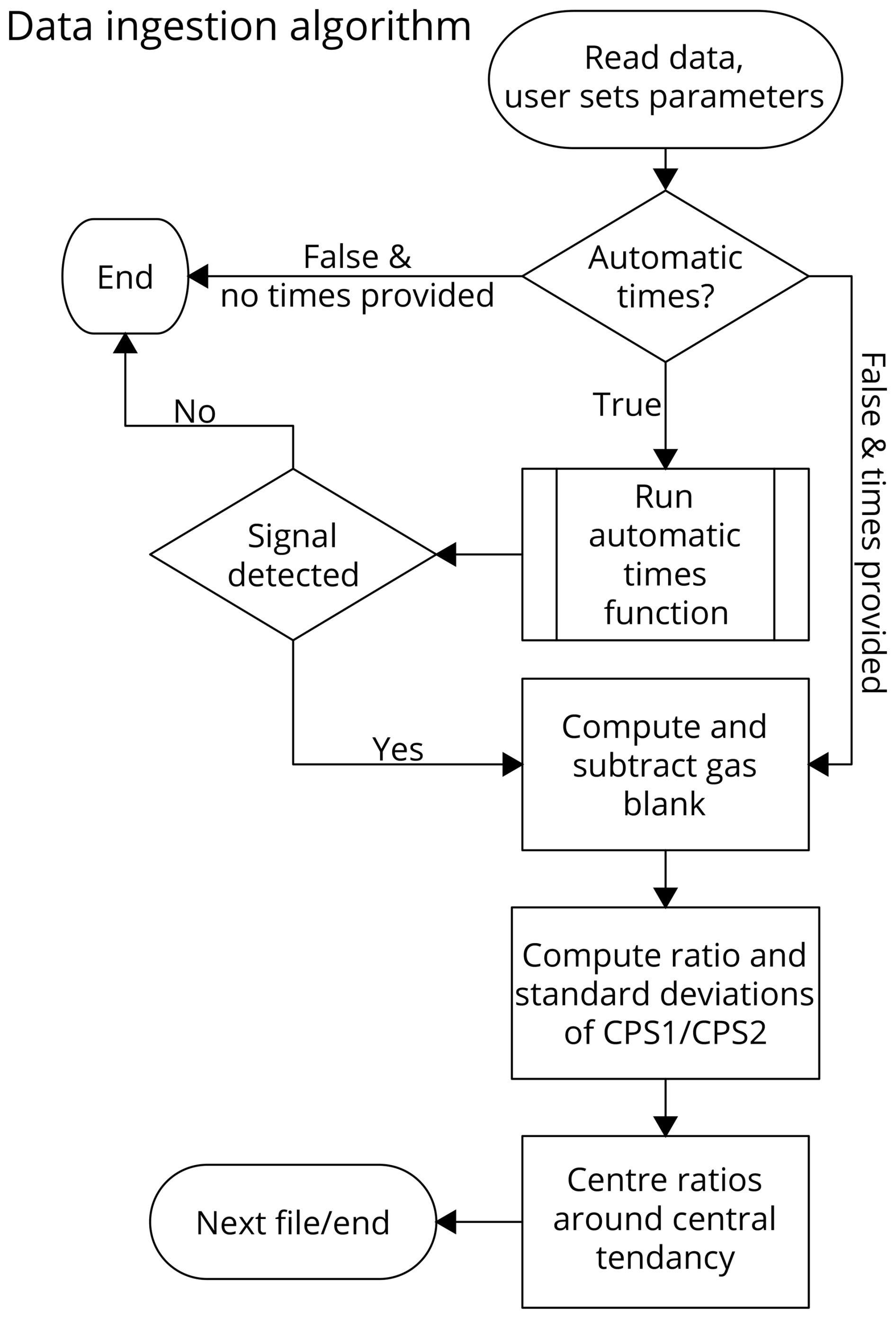
Figure 3 Outline of data ingestion algorithm. CPS = counts per second of analyte (e.g. ²³⁸U).

An automated procedure for determining gas blank and signal windows, as well as laser fire time, and aerosol arrival was developed to aid in rapid data processing and quality control. This algorithm is outlined at https://doi.org/10.25909/27041821 (Lloyd, 2024a, Fig. S1) with examples of the automatically determined time points and signal windows shown in https://doi.org/10.25909/27041821 (Lloyd, 2024a, Fig. S2).

Gas blank determination uses a geometric mean adapted for zeros (Eq. 1) as per Habib (2012):

$$\begin{array}{}\text{(1)}& \text{for}G\ge \mathrm{0},G={\displaystyle \frac{n_{+}{G}_{+}+n_{\mathrm{0}}G}{N}}={\displaystyle \frac{n_{+}}{N}}{G}_{+},\end{array}$$

where G is the geometric mean, N is the total count of data, x_i is the ith input value from i=1 to i=N, G₊ is the geometric mean of all x_i>0, n₊ is the count of x_i>0, G₀ is the geometric mean of all x_i=0 (i.e. 0), and n₀ is the count of all x_i=0.

As previously outlined (Sect. 2) the nature of orthogonal polynomial decomposition means that lambda coefficients (and their uncertainties) one and higher should not change with respect to a centred or non-centred dataset for a single analysis. For aggregated data (session and/or sample aggregation), higher-order lambda coefficients of centred and non-centred may not be equal unless all external factors (fluence, spot diameter, machine drift) have been controlled for. We strongly recommend that centred datasets are used for fitting intra- and intersession sample-aggregated datasets as the centring process will remove the influences of machine drift and tuning that λ₀ is sensitive to. Aggregation of data requires grouping by factors known to influence DHF (see Sect. 3.1) to ensure like-for-like data are being modelled.

Centring of the data aligns the central tendencies of each individual analysis to ≈1 while retaining the scale and shape (Fig. 4) of the change in raw ratios over the time-resolved signal, i.e. the DHF. Centring is performed by subtracting the central tendency (i.e. geometric mean, or a user could alternatively use the arithmetic mean, or median) from the time-resolved ratios for each individual file (i.e. analysis) and adding a constant value of 1.0 to the result. The addition of the constant to centre the values around one is to prevent numeric errors during weighted fits when the weights (input errors) are very small (i.e. close to 0). This centring enables visual comparison (Fig. 4) and accurate numeric assessment of DHF behaviours across samples, sessions, spot geometries, and fluences without the need to calibrate data to a known RM ratio for each session or accounting for machine drift during a session.

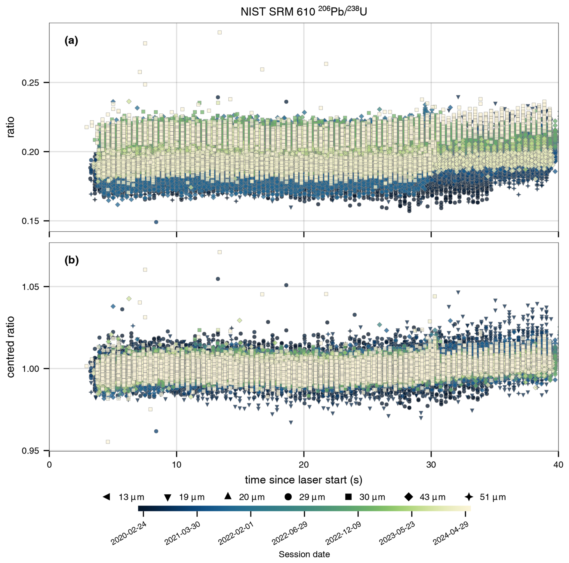
Figure 4 (a) Point-wise computed ${}^{\mathrm{206}}\mathrm{Pb}{/}^{\mathrm{238}}\mathrm{U}$ ratios for each measurement of NIST SRM 610 glass in the dataset. Symbol shapes represent spot diameter, and colour represents date of analytical session. (b) Centred, point-wise ${}^{\mathrm{206}}\mathrm{Pb}{/}^{\mathrm{238}}\mathrm{U}$ ratios for each measurement of NIST SRM 610 glass in the dataset (same data as in panel a). Centring (by subtraction of geometric mean and adding a constant of 1) preserves the relative positions of each data point but aligns them to a common central tendency. This preserves the shape and scale of the DHF pattern while removing ICP-MS tuning and drift effects, thus allowing accurate comparison between measurements using differing laser parameters, on different materials, and across ICP-MS sessions or laboratories.

2.2 Outline of fitting algorithm

In the following equations x denotes the independent variable (e.g. time in seconds) and the dependent variable (e.g. analyte ratio) is represented by y for observed values or $\widehat{y}$ for predicted values of some function of x, i.e. f(x). For clarity, we use φ to differentiate the orthogonal function terms and λ to differentiate the coefficients of the orthogonal polynomial from their regular counterparts (f and β, respectively). Function terms and coefficients use j and l as indices with k denoting the polynomial order. The indicator i is used for the ith value of x_i, y_i, and ${\widehat{y}}_i$ for i=1 to i=N (total count of data).

Polynomials of order k (Eq. 2) can be orthogonal to each other under some inner product (Eq. 3). The property of independence of each coefficient also enables efficient computation of the polynomial statistics (errors, variances and covariances, residual sum of squares, etc.) at each order. The efficient computation is enabled because only the coefficient matrix of the highest order (five in our case) needs to be calculated rather than the entire solution for each polynomial order. Once computed, subsequent calculations can use specific subsets of the operator and coefficient matrices to determine predictions and statistics for each polynomial order.

$$\begin{array}{}\text{(2)}& {\displaystyle }F\left(x\right)={\mathit{\beta }}_{\mathrm{0}}+\sum _{j=\mathrm{1}}^k\left[{\mathit{\beta }}_j{f}_j\left(x\right)\right]\text{(3)}& {\displaystyle }〈f_j\left(x\right),f_l\left(x\right)〉=\mathrm{0}\text{ for }j\ne l\text{(4)}& {\displaystyle }\mathrm{\Phi }\left(x\right)={\mathit{\lambda }}_{\mathrm{0}}+\sum _{j=\mathrm{1}}^k\left[{\mathit{\lambda }}_j{\mathit{\phi }}_j\left(x\right)\right]\end{array}$$

In this contribution, we apply this to the DHF observed during LA-ICP-MS using the orthogonal property in Eq. (5).

$$\begin{array}{}\text{(5)}& \sum \left[{\mathit{\phi }}_j\left(x_i\right){\mathit{\phi }}_l\left(x_i\right)\right]=\mathrm{0}\text{ for }j\ne l\end{array}$$

We construct a fourth-order polynomial function (Eq. 6) using the sum of a set of orthogonal polynomials (Anenburg and Williams, 2022; Bevington and Robinson, 2003; O'Neill, 2016).

$$\begin{array}{}\text{(6)}& \widehat{y}\left(x_i\right)={\mathit{\lambda }}_{\mathrm{0}}+{\mathit{\lambda }}_{\mathrm{1}}{\mathit{\phi }}_{\mathrm{1}}\left(x_i\right)+{\mathit{\lambda }}_{\mathrm{2}}{\mathit{\phi }}_{\mathrm{2}}\left(x_i\right)+{\mathit{\lambda }}_{\mathrm{3}}{\mathit{\phi }}_{\mathrm{3}}\left(x_i\right)+{\mathit{\lambda }}_{\mathrm{4}}{\mathit{\phi }}_{\mathrm{4}}\left(x_i\right)\end{array}$$

The orthogonal functions are solved for by using the methods outlined in Anenburg and Williams (2022) which make use of Vieta's formula and polynomial root finding. See Anenburg and Williams (2022), Appendix A, or the source code for further detail. Once the orthogonal polynomial forms are computed, the algorithm generates the operator matrix X and uses generalised least-squares regression (Eqs. 7 to 9) to solve the vector, λ, and matrix, U, while utilising analytical uncertainties (ϵ) for weights. The vector λ contains the polynomial coefficients λ₀…λ₄, while the matrix U contains the variances and covariances. Scaled values of ϵ are used to construct the diagonal values of the weight matrix Ω.

$$\begin{array}{}\text{(7)}& {\displaystyle }\mathit{y}=\mathbf{X}\mathit{\lambda }+\mathit{ϵ}\text{, }E\left[\mathit{ϵ}\mathrm{|}\mathbf{X}\right]=\mathrm{0}\text{, and }\text{Cov}\left[\mathit{ϵ}\mathrm{|}\mathbf{X}\right]={\mathit{\sigma }}^{\mathrm{2}}{\mathbf{\Omega }}^{-\mathbf{1}}=\mathbf{U}\text{(8)}& {\displaystyle }\mathit{\lambda }={\left({\mathbf{X}}^{\mathrm{T}}{\mathbf{\Omega }}^{-\mathbf{1}}\mathbf{X}\right)}^{-\mathrm{1}}{\mathbf{X}}^{\mathrm{T}}{\mathbf{\Omega }}^{-\mathbf{1}}\mathit{y}\text{(9)}& {\displaystyle }\mathbf{U}={\left({\mathbf{X}}^{\mathrm{T}}{\mathbf{\Omega }}^{-\mathbf{1}}\mathbf{X}\right)}^{-\mathrm{1}}\end{array}$$

A graphical representation of the individual orthogonal polynomial components and an example of the resulting fit is shown in Fig. 2. Our algorithm allows the user to employ automated outlier removal with an outlier considered to have a studentised residual ≥3. The residuals used in outlier identification are computed from the orthogonal polynomial order with the minimum Akaike information criteria corrected (AICc) value (Eq. 10) (Akaike, 1974; Burnham and Anderson, 2002). If outlier removal is enabled, the algorithm will iterate over the input data until no studentised residuals ≥3 remain in the fit or it has gone through 10 iterations. The minimum AICc is used to determine the “best fit” (i.e. minimum information loss) polynomial order for each dataset.

$$\begin{array}{}\text{(10)}& \text{AICc}=n\log \left({\displaystyle \frac{\text{rss}}{n}}\right)+\mathrm{2}k+{\displaystyle \frac{\mathrm{2}k\left(k+\mathrm{1}\right)}{n-k-\mathrm{1}}},\end{array}$$

where k is the order plus two, n is the count of data, and rss is the residual sum of squares for the model. Several measures of fit are computed and accessible to the user via the object created during the fitting algorithm. These measures include the Bayesian information criteria corrected (BICc), the AICc and BICc weights, the normalised root-mean-square error, the reduced chi-squared statistic ${\mathit{\chi }}_r^{\mathrm{2}}$, the multiple correlation coefficient ρ² or R² value, and an unbiased Olkin–Pratt-adjusted estimator ${\mathit{\rho }}_{\mathrm{OP}}^{\mathrm{2}}$ of ρ² (Karch, 2020; Olkin and Pratt, 1958). Further details on these measures of fit can be found in Appendix A.

An additional consideration in this algorithm is that floating point computation is inherently inexact, has finite precision, and can incur round-off errors (Fernández et al., 2003). While round-off errors are not an issue with most geochemical computations generally, due to the often small absolute values and numerous sequential computations being performed in this algorithm, these errors can lead to inaccuracy in the result. To overcome these potential accuracy issues we utilise the extended precision library MultiFloats.jl (Zhang, 2024) alongside Julia's native extended precision operations. We also use QR factorisation or singular value decomposition (SVD) depending on the condition number of the operator matrix to solve for the λ vector and the variance–covariance U matrix to ensure numeric stability. If, after the final calculation, the absolute value of a coefficient is less than the default machine rounding tolerance for the extended precision type (Float64x4), it is rounded to zero as it is considered to be unresolvable from a value of zero.

2.3 Analysis of reference materials by LA-ICP-MS

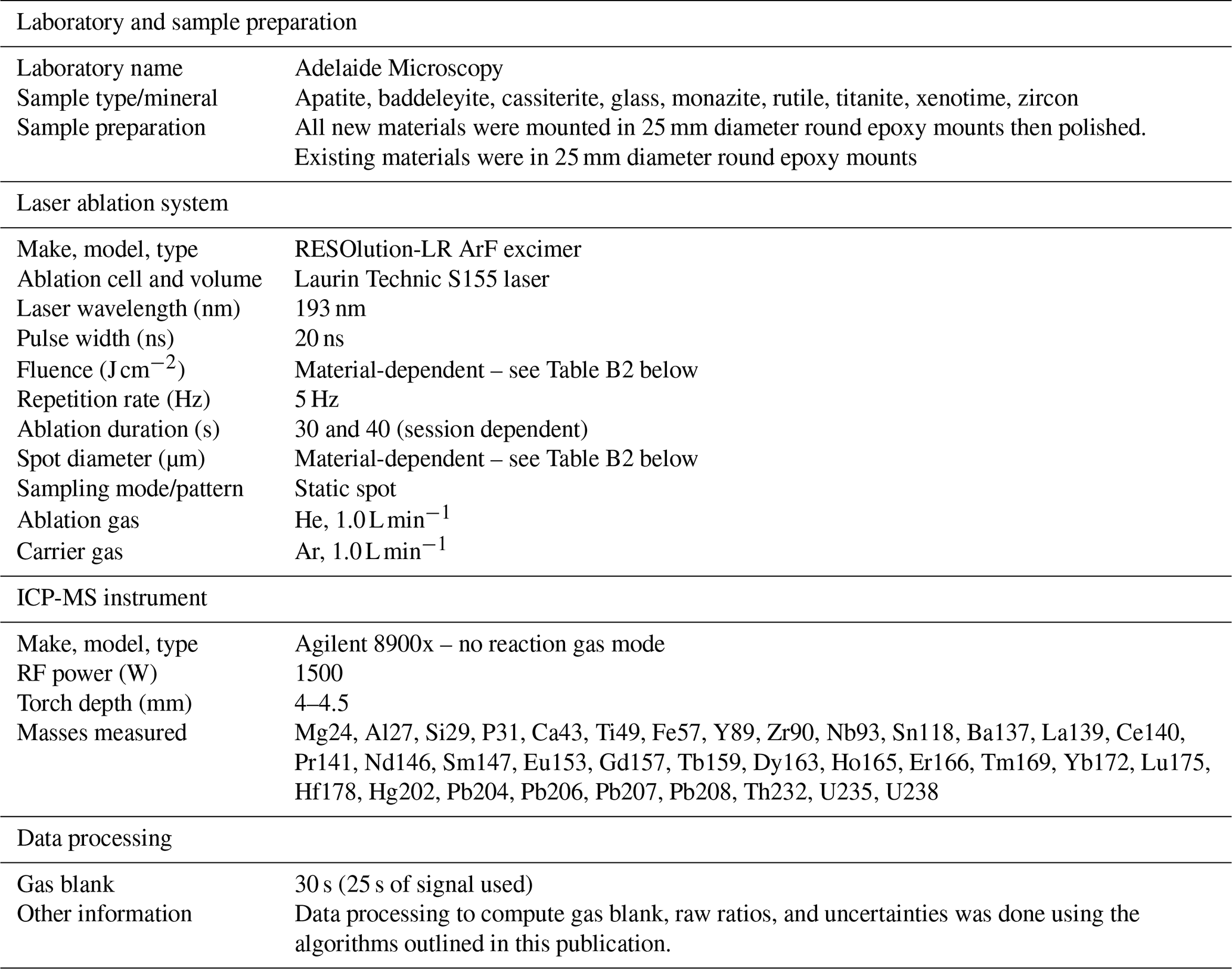
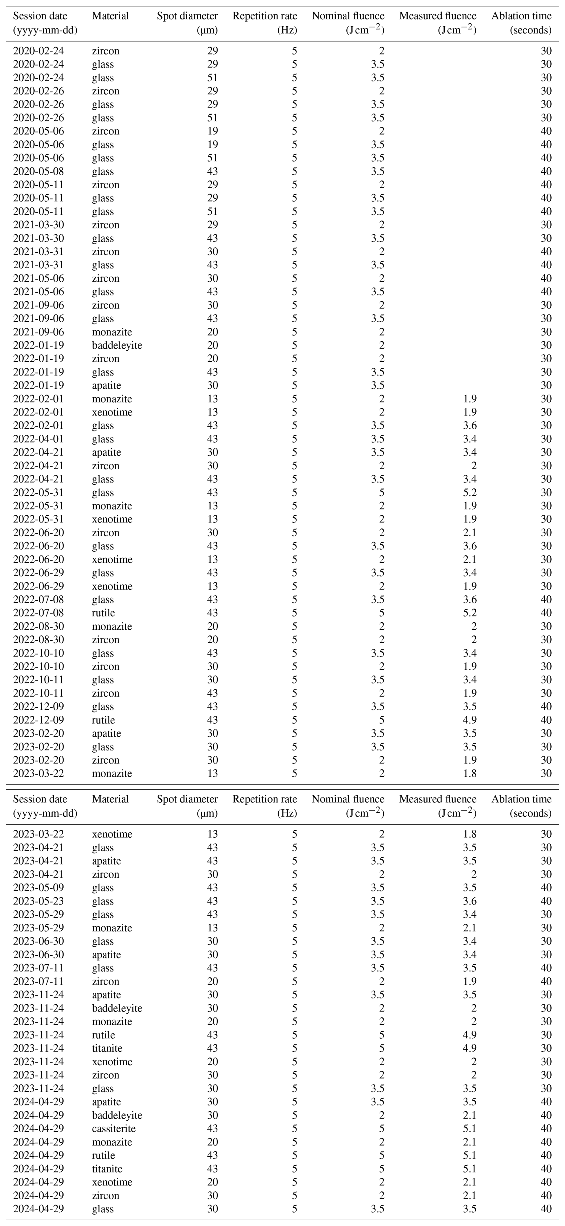
Reference materials for apatite (401, KO, MAD, Durango, Wilberforce), baddeleyite (BADPHE, G15874, G18650), monazite (TS1MNZ, 222, RW1, MAdel, MtGar, Ambat), rutile (R10, R19), titanite (Mt Painter, MKED), xenotime (MG1, BS1), and zircon (Mud Tank, Plešovice, GJ-1, 91500, Temora, Rak17) were analysed for U–Pb isotope ratios and trace element concentrations using optimal methods for the specific mineral (Bockmann et al., 2022; Fletcher et al., 2004; Gain et al., 2019; Glorie et al., 2020; Hall et al., 2018; Horstwood et al., 2016; Liu et al., 2011; Lloyd et al., 2022; Payne et al., 2008; Sláma et al., 2008; Spandler et al., 2016; Thompson et al., 2016; Wiedenbeck et al., 2004; Yang et al., 2024). An additional monazite (Pilbara) and several potential cassiterite (in-house) RMs were also measured. Samples were analysed using a RESOlution-LR 193 nm ArF excimer laser ablation system coupled to an Agilent 8900 ICP-MS/MS. Both instruments are housed at the University of Adelaide within the analytical facilities at Adelaide Microscopy. Full metadata for LA-ICP-MS analysis can be found in Appendix B.

Additional zircon, rutile, and baddeleyite RM data from prior studies were added to supplement the dataset and allow the assessment of the viability of inter-session comparisons (Lloyd et al., 2020, 2022, 2023, 2024; van der Wolff, 2020; Yang et al., 2024). These supplemental data were collected using the same LA system, coupled to either an Agilent 7900 ICP-MS (prior to November 2021) or the Agilent 8900 ICP-MS/MS in single quadrupole mode (from November 2021). Analytical conditions for these additional data can be found in the relevant references.

3 Results and discussion

In total, 5478 analyses (CSV files) were processed and their DHF patterns were modelled with the orthogonal polynomial decomposition outlined above (Sect. 2.2). This results in 5478 analysis fits, 188 session fits (sample aggregated per session), and 58 sample fits (sample aggregated across all sessions) accounting for differences in spot geometry across 29 unique materials (Figs. 5 and 6).

Linear slopes for the sample fits (λ₁) range from $-\mathrm{5.88}\times {\mathrm{10}}^{-\mathrm{5}}$ to 0.0217 s⁻¹, quadratic curvatures (λ₂) range from $-\mathrm{3.06}\times {\mathrm{10}}^{-\mathrm{5}}$ to $\mathrm{3.27}\times {\mathrm{10}}^{-\mathrm{5}}$ s⁻², cubic curvatures (λ₃) range from $-\mathrm{9.76}\times {\mathrm{10}}^{-\mathrm{6}}$ to $\mathrm{1.91}\times {\mathrm{10}}^{-\mathrm{5}}$ s⁻³, and quartic curvatures (λ₄) range from $-\mathrm{4.23}\times {\mathrm{10}}^{-\mathrm{6}}$ to $\mathrm{3.82}\times {\mathrm{10}}^{-\mathrm{7}}$ s⁻⁴. Given the small numbers and large quantity of fits, it is not feasible to display a table with all parameters nor is it intuitive for the reader. Instead, we provide the visual representation of λ₁ plotted against λ₂ and their best fit uncertainties (2 standard error) in Fig. 5, as well as the visual polynomial fit and its uncertainty for the sample fits in Fig. 6.

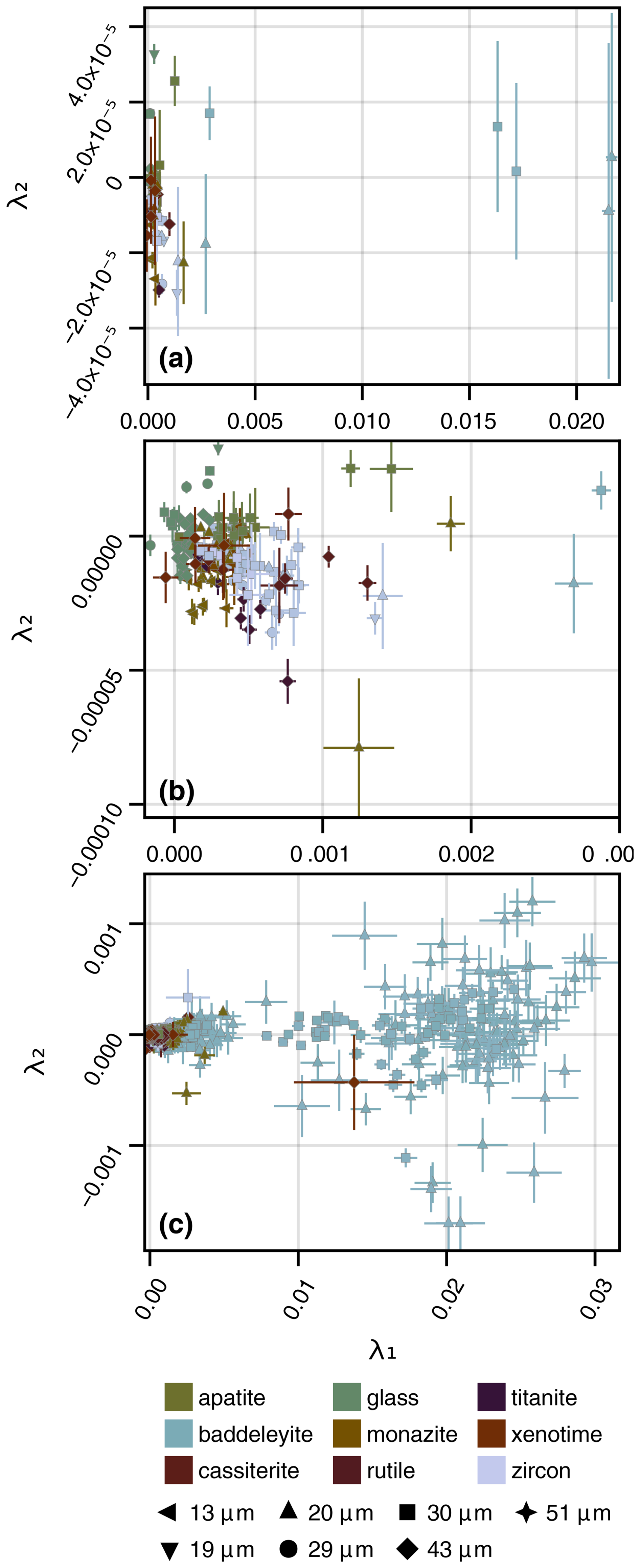
Figure 5 Scatter plot of λ₁ (x axis) and λ₂ (y axis) for sample-aggregated (a), session-sample-aggregated (b), and individual analysis (c) orthogonal polynomial fits. Symbol shapes represent spot diameter, and symbol colour represents material type. Uncertainty bars are 2 standard error. Fits with a greater positive linear slope will plot further to the right, and fits with a greater quadratic curvature will plot to higher (positive) or lower (negative) positions on the y axis. In these simple bi-plots it can be readily observed that distinguishing between points becomes difficult or near impossible when many data are plotted or there is large variation in some data.

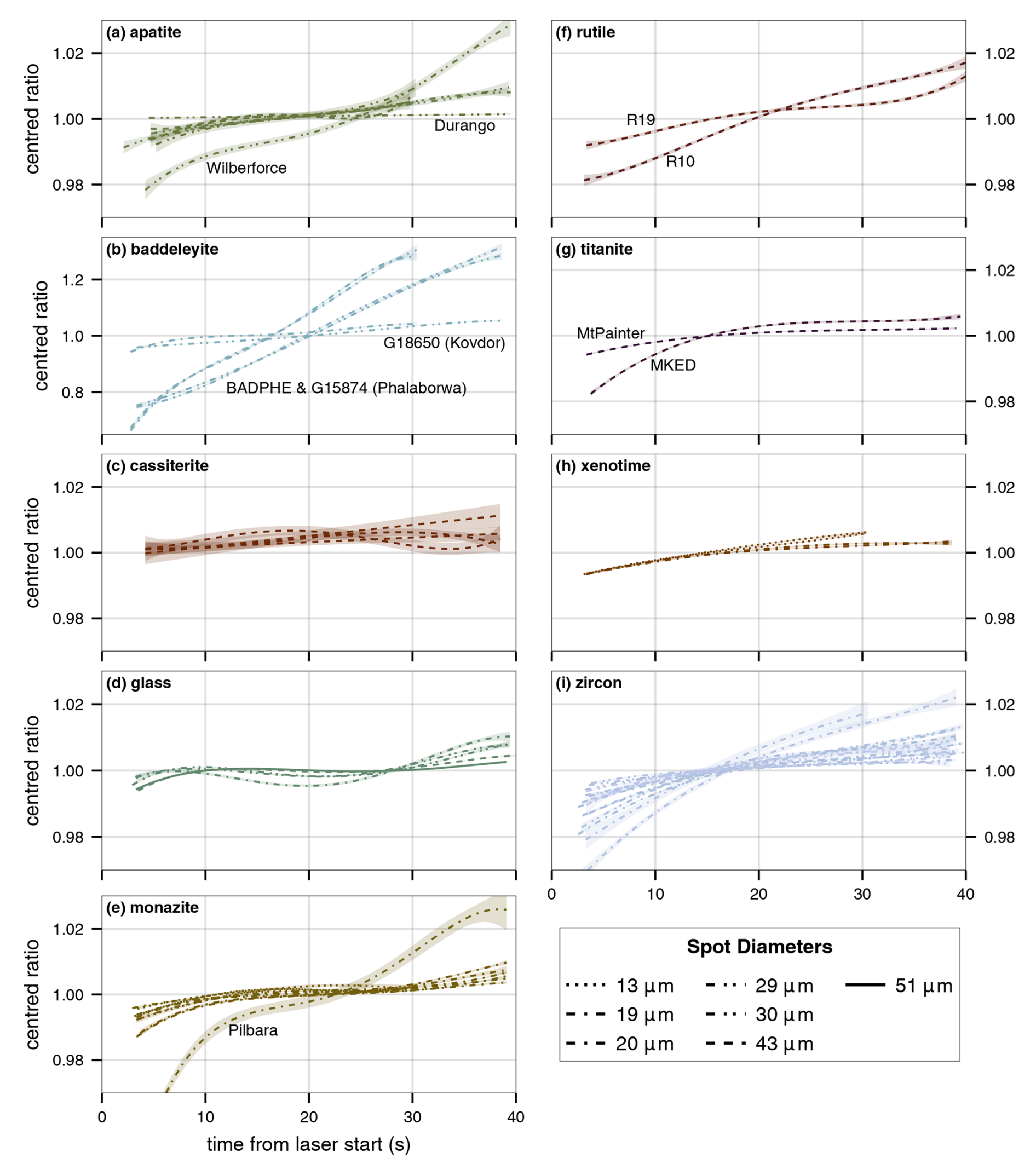
Figure 6 Orthogonal polynomial fits of down-hole fractionation (${}^{\mathrm{206}}\mathrm{Pb}{/}^{\mathrm{238}}\mathrm{U}$) grouped by sample material. Note that the baddeleyite has a significantly larger y-axis scale due to the steeper linear fractionation component. Shaded areas show the 95 % confidence interval of the individual fit. Increasing line solidity corresponds to increasing spot diameters.

3.1 Factors affecting down-hole fractionation

The scope of this contribution is to provide a tool that can be used for quantitative modelling of DHF and not an assessment of factors that influence DHF. Nonetheless, it is worth highlighting what the influencing factors are and what considerations are needed for accurately using the proposed method to model these patterns. As stated earlier, DHF is a phenomenon observed in LA-ICP-MS (and other mass-spectrometry methods) where the observed inter-element isotopic ratios change as a function of ablation depth/time independent of geological heterogeneity. This phenomenon is known to have several contributing factors, and their interactions are complex (Guillong and Günther, 2002; Günther et al., 1997; Hergenröder, 2006a, b; Horn et al., 2000; Košler et al., 2005; Kroslakova and Günther, 2006; Mank and Mason, 1999; McLean et al., 2016; Paton et al., 2010; Sylvester and Ghaderi, 1997; Ver Hoeve et al., 2018). It is known that sample material, spot diameter–depth ratio/geometry, laser wavelength, fluence, laser repetition rate, and analyte volatilities all noticeably influence the observed down-hole inter-element isotopic ratio. Thus, careful consideration of these parameters is needed when performing any modelling of the observed patterns. For example, it would not be sensible to combine data from two analyses of the same material that have different laser repetition rates and model that combined data, as a priori knowledge dictates that we would observe different DHF patterns over the same time interval from the two separate analyses. As such, when aggregating data in this current study, we ensure that only like-for-like data are combined, e.g. same material using the same laser wavelength with the same laser parameters (spot geometry, repetition rate, fluence) within a small tolerance (e.g. nominally 2.0±0.1 J cm⁻²). Future studies could assess what a suitable tolerance is for each parameter; however, tolerances used in the current study (e.g. ±0.1 J cm⁻²) do not appear to cause spurious results.

3.2 Physical interpretation of λ coefficients

Without needing RM calibration, the derived coefficients (λ₁ and higher) represent numerical parameters of DHF patterns for any given analysis (Fig. 2).

The first coefficient, λ₀, will inherit the units of the y variable. For this study, the value is unitless due to the y variable being $\frac{\text{CPS}}{\text{CPS}}$ but can be interpreted as the mean of y, i.e. the mean ratio. As we are centring all data around a value of one to remove the influence of machine calibration and drift, λ₀ has limited use in this research contribution; however, it could be used to calculate machine drift, and the nominal correction value for known-ratio materials (ICP-MS mass-bias correction) during data reduction. The second coefficient, λ₁, has units of s⁻¹ and can be interpreted as the average rate of change/overall magnitude of change of the ratio between two analyte intensities over time. We suggest that this component largely reflects the fractionation occurring as a result of the change in depth-to-radius ratio during ablation. The third coefficient, λ₂, has units of s⁻² and can be interpreted as the acceleration (or deceleration) in the rate of change of the ratio over time. We propose that fractionation due to differences in the relative volatilities of the analytes is the major control on this component, i.e. the analyte signal intensities decaying at different rates as the depth-to-radius ratio increases.

Higher-order terms have more complex meanings: they are subsequent derivatives of the prior term. The fourth coefficient, λ₃, has units of s⁻³ and can be interpreted as the rate of change in the acceleration (λ₂) of the ratio rate of change through time. This is likely reflecting the focussing of the laser-induced plasma as the hole geometry changes and causes the subsequent change in shape of the ablation plume from the ablation site. It will be represented by an inflection point in the signal (i.e. free surface expansion to increased crater wall interaction). The fifth coefficient, λ₄, has units of s⁻⁴ and can be interpreted as the rate of change of λ₃ over time. We believe this term could be incorporating detector effects such as electrical noise, low signal-to-background ratios, and Poisson noise at low signal intensity.

From the above reasoning, we expect that a third-order polynomial (Φ₃(x), λ_1…3) should account for most of the variation seen in ratios over time during static spot ablation as a function of the ablated material and measured analytes. The fifth term (fourth-order polynomial) should incorporate the remaining contributions to the fit that are likely to be a result of instrument-induced artefacts.

3.3 Data analysis and visualisation

The proposed algorithm can efficiently handle large datasets, generating substantial numeric data. This presents two challenges: (1) analysing the data as it becomes a “big data” problem and (2) visualising the data in a meaningful and interpretable way.

There exists well-established literature for the analysis of large and/or multidimensional datasets. For multivariate data there is often a transformation from a higher-dimensional space to a lower-dimensional space to enable univariate and bivariate statistics. For example, methods such as principal component analysis (PCA) may be used to numerically evaluate the multivariate datasets.

Visualisation of multidimensional and/or large datasets is challenging. For simple 2-D data, an analyst can produce bi-plots (x–y scatter plots) to visualise any relationships in data. For 3-D and 4-D data, analysts can plot either ternary or quaternary diagrams which require mathematical transformations of the data into a lower dimension (e.g. 3-D to 2-D) that emulates the higher-order space; hence, they are increasingly complex to visualise and interpret. In all cases large datasets can lead to visual clutter (over-plotting) where the viewer will not be able to readily distinguish between similarly positioned data points.

In Fig. 5 we have plotted λ₁ on the x axis and λ₂ on the y axis, with corresponding uncertainty bars (2 SE). These plots are limited to displaying only two of the five coefficients and suffer from visual clutter where it is difficult to distinguish some point from another and from scaling issues where the variation in some data is responsible for obscuring the view of other data.

Alternatively an analyst can employ dimensional reduction visualisation methods such as PCA, multidimensional scaling (MDS), or uniform manifold approximation and projection (UMAP) to visualise the higher-dimensional data in a lower-dimensional space. PCA can still incur visual clutter as multiple reduced components may still share the same coordinates, and PCA may not always be able to reduce the data to only two or three principal components that explain the majority of variance in a dataset. Conversely, UMAP will always be able to reduce a dataset to a specified number of dimensions and has hyperparameters that enhance visualisation to eliminate visual clutter.

We utilise UMAP (Fig. 7) to visualise the relative relationships of the higher-dimensional data in a lower-dimensional space (McInnes et al., 2020). UMAP takes the input multidimensional data (5478×4 λ coefficients in this study) and tries to find a common embedding space (using the manifold assumption) to represent the local and global data topology in a lower dimension. UMAP has several variables called hyperparameters which control the output of the algorithm. The n-nearest neighbours hyperparameter is the most important for finding the balance between the global (low n-n) and local (high n-n) data structure. We use a value of 19 for the n-nearest neighbours hyperparameter as the minimum number of analyses for a single material in a session is 20, so we expect there to be 19 related points. We set the minimum distance hyperparameter to 1.0 to push the points apart to help visualisation.

In simpler terms, UMAP works by constructing a graph in high-dimensional space (e.g. 4-D) that is projected onto a lower-dimensional space (e.g. 2-D) where points are connected based on their closeness in higher-dimensional space. The shape of the data clusters in UMAP is a manifestation of the spatial relationships between higher-dimensional data with similar attributes and is not directly interpretable in a physical manner like traditional bi-plots or PCA (McInnes et al., 2020).

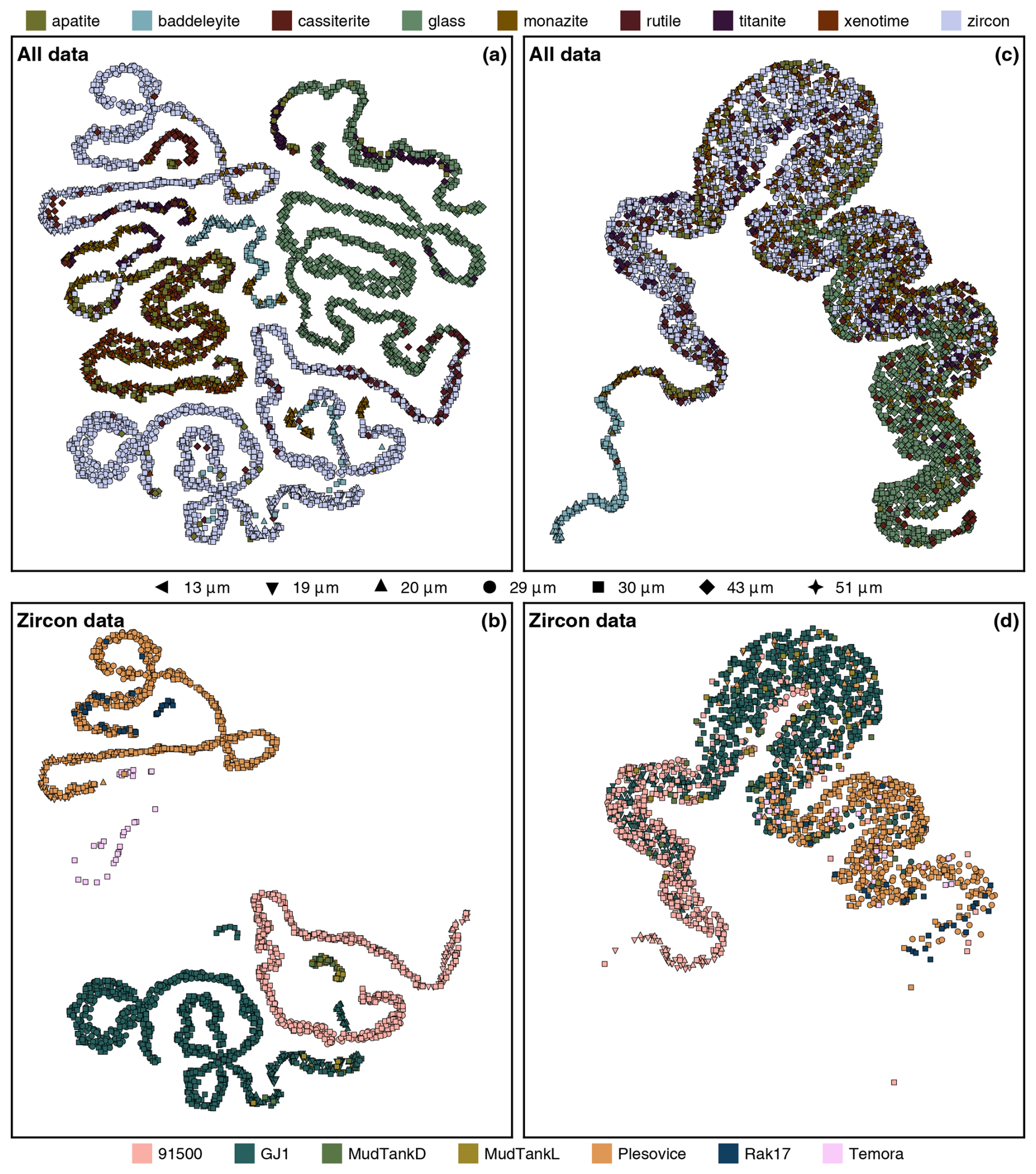
Figure 7 (a) Uniform manifold approximation and project (UMAP) of λ coefficients 0 to 4 for all analysis data (non-centred) in the study. (b) Subset of (a) only including zircon analyses. (c, d) UMAP of λ coefficients 1 to 4 for centred analysis data in the study with (d) being the zircon data subset of (c). In a practical sense, the closer or more clustered the points are to each other, the more similar they are. Axes are omitted, as x–y coordinates are a normalised distance metric value with no physical meaning. This method of data visualisation is to help an end user understand the relative similarities within large datasets. Panels (a) and (b) are strongly controlled by the λ₀ component, while (c) and (d) are reflecting the shape parameters λ_1…4 of different materials.

3.3.1 Interpreting the (sample-aggregated) data fits

Oxides generally have a greater linear slope component (λ₁) compared to other materials analysed, cassiterite being an exception (Figs. 5 and 6). The glass (NIST SRM 610), cassiterite, and xenotime samples show the least overall DHF. Of note with the glass (NIST SRM 610) is we can clearly see the impact of spot diameter (thus geometry) on DHF. With decreasing spot diameter, the overall magnitude (linear slope) of DHF is increased (Fig. 6), but it also exacerbates the complex shape parameters (quadratic and cubic curvatures, etc.).

There are two distinct groupings (accounting for different spot diameters) for baddeleyite, with one group being the samples from Phalaborwa and the other group being the Kovdor sample (Fig. 6). The cause of this stark disparity in baddeleyite DHF is unknown, but the Ti concentration is 9–14 times higher in the Phalaborwa samples than in the Kovdor samples. The obvious outliers in the apatite, cassiterite, and monazite panels of Fig. 6 are the Durango and Wilberforce apatite samples, CstT4370 cassiterite, and the Pilbara monazite sample. For the Pilbara monazite, some analyses show considerable variation in their Pb and U concentration (proxied by count rate; see the “Code and data availability” section for signal plots available at figshare). Excluding these analyses from the sample/session aggregated fit for the Pilbara monazite will reduce the polynomial confidence interval and would improve the quality of the fit. However, these data are still analytically relevant and indicate that the Pilbara monazite may not be suitable to be an RM due to the variable ratio of Pb and U. For the Durango apatite, the flat DHF fit and larger uncertainty are due to low Pb counts, and for Wilberforce, the steeper linear DHF component and larger uncertainty are due to the inclusion of several points from some analyses that are highly leveraging the fit, even with automated outlier removal being applied. For cassiterite, the relatively flat fits and outlier (CstT4370) are generally due to low Pb and/or U counts and greater scatter in the underlying data. The discrepancies and/or larger uncertainties in the lambda coefficients for materials of the same type provide a way to numerically check for outliers in RM data, prior to further data reduction, rather than needing a user to review all the data graphically. A user should still review their data via graphical means as well to check for spurious results.

3.3.2 Application of UMAP as a data visualisation aid

For this study, a UMAP diagram (Fig. 7) helps to visualise the relative similarities between the λ coefficients for the 5478 analyses. If there are relationships in the data, we expect them to correlate with the individual materials (e.g. NIST SRM 610 glass, GJ-1 zircon, Plešovice zircon), the type of material (e.g. glass, zircon, xenotime), laser parameters, or a combination of these factors and thus plot in clusters on a UMAP diagram. The resulting map (Fig. 7) clearly differentiates the various materials better than the simple bi-plot (Fig. 5c), which suffers from over-plotting, obscuring any similarities/trends. The UMAP algorithm was not provided prior knowledge about the material, only the λ coefficients. Panels (a) and (b) of Fig. 7 are strongly controlled by the mean ratio (λ₁) as the UMAP algorithm was provided with lambda values from non-centred fits to aid the reader in understanding the general principle of these diagrams. Panels (c) and (d) of Fig. 7 are more useful in visualising the relationships of the shape parameters within the DHF models as the effects of mass bias and drift are removed by providing the algorithm with the lambda values from centred fits.

For small, simple datasets, a simple bi-plot may suffice, but in larger datasets, and especially an inter-laboratory comparison where there is likely to be several hundreds of thousands to millions of individual data points, a method such as UMAP should be employed to visualise the relationships of the data.

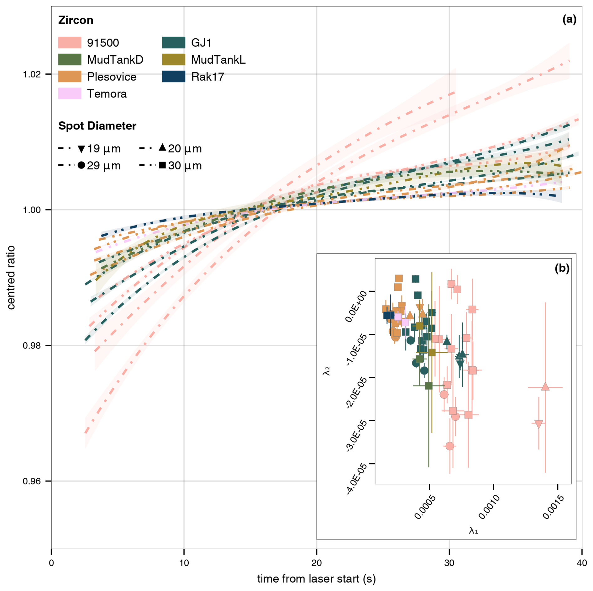
Figure 8 (a) Orthogonal polynomial fitting of down-hole fractionation for zircon data in this study. The visualised polynomials represent the best-order fit for the aggregated data of a given sample at a single spot diameter, e.g. GJ-1 at 30 µm, GJ-1 at 19 µm. Shaded areas show the 95 % confidence interval of the individual fit. The inset graph (b) shows the λ₁ and λ₂ coefficients and their 2 standard error uncertainty for each of the session-based fits for the seven zircons analysed. Fits with a greater linear slope plot further to the right, and fits with a greater negative quadratic curvature (i.e. the slope flattens at a faster rate) will plot toward the bottom.

In Fig. 7, it is apparent that baddeleyite (pale blue-green markers in the upper panels) DHF is different to all other materials analysed in this study as the points are forming their own clusters (particularly Fig. 7c). The deviation by baddeleyite is also reflected in Fig. 5 where baddeleyite analyses are plotting to the far right of each subplot, indicating a much stronger linear slope fractionation component. What is also noticeable is that there is a large diversity in the DHF patterns of zircon (Fig. 7b and d), which in part is due to analytical noise as the individual points represent a single analysis and the fits have greater uncertainty as they are more susceptible to that noise. Nevertheless, in general 91500 is behaving most differently from all other zircons at a given spot diameter (Fig. 8), and Plešovice is behaving most like NIST SRM 610 of all the zircons (Fig. 7c and d). We do not suggest that NIST SRM 610 glass is a suitable alternative to correct DHF for zircon (as seen in Figs. 6 and 1), rather that there is significant variation in the DHF of zircon standards, and therefore careful consideration should be given to applying appropriate zircon standards for analytical sessions depending on the unknown zircons to be analysed and the time period used for signal integration (Guillong and Günther, 2002; Hergenröder, 2006a; Košler et al., 2005; Paton et al., 2010).

We can see that spot geometry has a significant impact on DHF (Fig. 6, glass and zircon panels; Figs. 7 and 8), which is a known phenomenon (Horn et al., 2000; Mank and Mason, 1999; Paton et al., 2010). However, all zircons except 91500 have remarkably similar DHF patterns at 29 µm (and 30 µm) (Fig. 8). The linear slope component (λ₁) of the DHF pattern appears to be relatively constant between laser sessions for a given zircon and spot diameter, while the quadratic component varies (Fig. 8b) but has greater uncertainty associated with it. The exact mechanism as to why 91500 shows greater DHF than the other analysed zircons is unknown and not the focus of this paper; however, prior studies have investigated the potential causes of differing DHF patterns in zircon and glass (Košler et al., 2005), and it is possible that radiation damage plays a role (Allen and Campbell, 2012; Marillo-Sialer et al., 2014; Solari et al., 2015; Thompson et al., 2018).

3.4 Applications

The algorithm defined in this paper offers a way to numerically quantify processes in geoscience that can be modelled with a linear combination of basis functions, building on the work of O'Neill (2016) and Anenburg and Williams (2022) with a more generalised approach. The generalised nature of this algorithm allows it to be used for orthogonal polynomial fitting, up to fourth order, of any data where it is sensible; i.e. there exists a polynomial of order k_(0…4) that can model the input data. In this contribution we use it to numerically quantify DHF patterns of varied materials during LA-ICP-MS and demonstrate UMAP as a visualisation technique to help understand the structure of the data.

We envisage that this algorithm could be implemented in data reduction software to self-correct the DHF pattern of well-behaved materials (i.e. fitting a single geochemical zone) or as splines to geologically meaningful zonation, with a fallback to a known homogeneous material where the analysis signal is complex (e.g. due to complex zonation or inclusions). In the latter case, the user would need to select an appropriate material, and it would likely result in somewhat inaccurate correction in any case, thus impacting the accuracy of the final result (Fig. 1). Self-correction would require modelling the individual analysis signal and using the orthogonal model to then correct the data for DHF observed in that analysis.

Alternatively the coefficients of the orthogonal models could be used to determine which RM DHF pattern best suits the unknown material DHF pattern. The quantification of the DHF pattern enables numeric assessment of fits to unknowns against fits of knowns to find the most similar material with respect to DHF and of the appropriate model order. For example, the AICc is minimised for the fourth-order polynomial for NIST SRM 610 and the third-order polynomial for most zircon RMs, and we can see this reflected visually in Figs. 2, 4, 6, and 8. Using the measures of fit provides users with a way to choose an appropriate model that accurately reflects the uncertainty and scatter while minimising overfitting and the introduction of artefact errors. Additionally, the quantification done by this algorithm provides a way for laboratories to quantitatively compare the DHF behaviour of their RMs and analytical setup against other laboratories.

4 Conclusions

This contribution generalises the orthogonal polynomial decomposition algorithms of O'Neill (2016) and Anenburg and Williams (2022) to allow for modelling of processes in geoscience that can be represented by a linear combination of basis functions (predictable x-to-y relationships) beyond rare earth element (REE) patterns while also using input uncertainties as weights for the models. Being written in the Julia programming language enables fast computation of many thousands of input files from data ingestion to model output.

We demonstrate quantitative modelling of DHF patterns observed during static spot LA-ICP-MS using the developed algorithm by applying it to an exemplar dataset of U–Pb RMs and guide the reader through data visualisation and interpretation of the derived coefficients. The algorithm provides the ability to quantitatively compare DHF for the same RMs across laboratories, differences between RMs, and differences between analytical setups.

Furthermore, this algorithm could be implemented into data reduction programmes to numerically assess the similarities and fit qualities of DHF correction, ensuring more accurate corrections are made. It is possible that the algorithm could be used to self-correct the DHF pattern of a single analysis by first modelling it and then using that model to correct the pattern so long as the assumption that the signal (or portion of) reflects a single, geologically meaningful zone holds. This allows a relaxation of the assumption that the DHF pattern of an unknown is the same as a specified RM by decoupling the correction from that material which can lead to improvements in accuracy and/or precision of the final result. More conservatively or in cases where the assumption of a single geologically meaningful zone does not hold, models of the individual analyses can be used to quantitatively choose the most similar RM to use as a DHF correction material.

Appendix A: Algorithmic mathematics

LA-ICP-MS count data are strictly positive integers and follow a (discrete) Poisson distribution at low count level (e.g. gas blank), although they eventually approximate a normal distribution at high count rate as implied by the central limit theorem (Bevington and Robinson, 2003). Data from a mass spectrometer used for geochronology and/or elemental analysis are generally output in counts-per-second (CPS), not counts, and violate the integer requirement of a discrete probability distribution. This combined with the less intuitive and asymmetric scale parameters of geometric means has led to the use of normal statistics (e.g. arithmetic means) for ratio computations. The use of normal statistics for gas blank measurements generally leads to overestimation (arithmetic mean) or underestimation (median if lots of 0 counts) and to a violation of the equality $A/B={\left(B/A\right)}^{-\mathrm{1}}$. This latter violation is commonly seen in U–Pb geochronology, where ${}^{\mathrm{206}}\text{Pb}{/}^{\mathrm{238}}\text{U}\ne {\left({}^{\mathrm{238}}\text{U}{/}^{\mathrm{206}}\text{Pb}\right)}^{-\mathrm{1}}$. Given that elemental count data and elemental ratios are compositional data and are strictly positive real values (i.e. positively skewed) which often follow a log-normal distribution, a geometric mean is a more appropriate measure of the central tendency of the data. In our algorithm we use the geometric mean to compute the gas blank value. While geometric means are often used to address the problems above, we use a modified geometric mean to incorporate valid zero values which a standard geometric mean cannot. We will first review the standard geometric mean before detailing the modified version. The geometric mean is defined for a set of positive real numbers as Eq. (A1) (Habib, 2012; Feng et al., 2017):

$$\begin{array}{}\text{(A1)}& G=\sqrt[N]{\prod _{i=\mathrm{1}}^N{x}_i},\end{array}$$

where G is the geometric mean, N is the total count of data, and x_i is the ith input value from i=1 to i=N. Alternatively, it can be calculated by the arithmetic mean of the logarithm of the values (Eq. A2) and then raising the result to e (Eq. A3) (Habib, 2012; Kirkwood, 1979; Feng et al., 2017).

$$\begin{array}{}\text{(A2)}& {\displaystyle }\log G={\displaystyle \frac{\mathrm{1}}{N}}\sum _{i=\mathrm{1}}^N\log x_i\text{(A3)}& {\displaystyle }G=e^{\log \left(G\right)}\end{array}$$

As computing the product of an arbitrarily large series of numbers can lead to overflow errors (Fernández et al., 2003; Polhill et al., 2006) and therefore inaccurate results, most geometric mean algorithms implement the second form where the arithmetic mean is calculated from the logarithm-transformed data and raised to e. The logarithmic transformation requires that all x_i>0. Additionally, as this is a multiplicative mean, when any x_i=0, G=0.

To overcome these limitations and obtain a more accurate estimate of the mean gas blank, we implement a geometric mean that accounts for zeros (Eq. A4). This equation is effectively a weighted arithmetic mean of the geometric mean of the values >0, and the geometric mean of the zeros, i.e. 0, with the weights equal to the number of values in each category (Habib, 2012):

$$\begin{array}{}\text{(A4)}& \text{for }G\ge \mathrm{0}\text{, }G={\displaystyle \frac{n_{+}{G}_{+}+n_{\mathrm{0}}{G}_{\mathrm{0}}}{N}}={\displaystyle \frac{n_{+}}{N}}{G}_{+},\end{array}$$

where G₊ is the geometric mean of all x_i>0, n₊ is the count of x_i>0, G₀ is the geometric mean of all x_i=0 (i.e. 0), and n₀ is the count of all x_i=0. While this form of the geometric mean has its critics (de la Cruz and Kreft, 2018), we believe it provides a more accurate estimate of the true gas blank which should lie somewhere between 0 and the arithmetic mean which will bias the result to values >0, and it avoids the issue of small constants being added to the data causing major changes in the geometric mean (Feng et al., 2017).

Although they cannot handle values of zero, we implement a geometric variance (Eq. A5), geometric standard deviation (Eq. A6), and standard error of the geometric mean (Eq. A7) (Kirkwood, 1979; de Carvalho, 2016):

$$\begin{array}{}\text{(A5)}& {\displaystyle }\text{for }x>\mathrm{0}\text{, }{\mathit{\sigma }}_G^{\mathrm{2}}=e^{{\mathit{\sigma }}_{\log x}^{\mathrm{2}}},\text{(A6)}& {\displaystyle }\text{for }x>\mathrm{0}\text{, }{\mathit{\sigma }}_G=e^{\mathit{\sigma }\left(\log x\right)},\text{(A7)}& {\displaystyle }\text{for }x>\mathrm{0}\text{, }{\text{SE}}_G=e^{S{E}_{\log x}},\end{array}$$

where ${\mathit{\sigma }}_{\log x}^{\mathrm{2}}$, σ_log x, and SE_log x are, respectively, the variance, standard deviation, and standard error of the mean of the logarithms of x_i>0. The σ(log x) can also be interpreted as the average magnitude of the relative deviation from the geometric mean and SE_log x (Chatfield et al., 2025). In geometric statistics, the measures of variance, standard deviation, and standard errors are scale parameters. The corresponding uncertainty range of G for these statistics is asymmetric and denoted by $\left(G\times u;G÷u\right)$, where u is the corresponding statistic (e.g. σ², σ, SE).

A1 Orthogonal polynomial decomposition

We use orthogonal polynomial decomposition to fit a polynomial to analyte ratio data where the coefficients have physical meaning in relation to those data. This decomposition enables quantification of the shape parameters of a down-hole fractionation pattern. Integral to this process is the calculation of the orthogonal polynomials (Eq. A8) to be used to fit the final model.

$$\begin{array}{}\text{(A8)}& \widehat{y}\left(x_i\right)={\mathit{\lambda }}_{\mathrm{0}}+{\mathit{\lambda }}_{\mathrm{1}}{\mathit{\phi }}_{\mathrm{1}}\left(x_i\right)+{\mathit{\lambda }}_{\mathrm{2}}{\mathit{\phi }}_{\mathrm{2}}\left(x_i\right)+{\mathit{\lambda }}_{\mathrm{3}}{\mathit{\phi }}_{\mathrm{3}}\left(x_i\right)+{\mathit{\lambda }}_{\mathrm{4}}{\mathit{\phi }}_{\mathrm{4}}\left(x_i\right)\end{array}$$

Our implementation can fit up to a fourth-order polynomial and requires solving the orthogonal property of Eq. (A9) for each orthogonal function, φ(x).

$$\begin{array}{}\text{(A9)}& \sum \left[{\mathit{\phi }}_j\left(x_i\right){\mathit{\phi }}_k\left(x_i\right)\right]=\mathrm{0}\text{for }j\ne k\end{array}$$

The functions φ_1…4 are as follows.

$$\begin{array}{c}{\displaystyle }{\mathit{\phi }}_{\mathrm{1}}=x_i-\mathit{\beta }\\ {\displaystyle }{\mathit{\phi }}_{\mathrm{2}}=\left(x_i-{\mathit{\gamma }}_{\mathrm{1}}\right)\left(x_i-{\mathit{\gamma }}_{\mathrm{2}}\right)\\ {\displaystyle }{\mathit{\phi }}_{\mathrm{3}}=\left(x_i-{\mathit{\delta }}_{\mathrm{1}}\right)\left(x_i-{\mathit{\delta }}_{\mathrm{2}}\right)\left(x_i-{\mathit{\delta }}_{\mathrm{3}}\right)\\ {\displaystyle }{\mathit{\phi }}_{\mathrm{4}}=\left(x_i-{\mathit{\epsilon }}_{\mathrm{1}}\right)\left(x_i-{\mathit{\epsilon }}_{\mathrm{2}}\right)\left(x_i-{\mathit{\epsilon }}_{\mathrm{3}}\right)\left(x_i-{\mathit{\epsilon }}_{\mathrm{4}}\right)\end{array}$$

Here β, γ_n, δ_n, and ε_n are predetermined constants calculated prior to fitting the final model. The solution to β is simply the arithmetic mean of the x values (Eq. A10).

$$\begin{array}{}\text{(A10)}& \sum _{i=\mathrm{1}}^N\left(x_i-\mathit{\beta }\right)=\mathrm{0}\text{, leading to}{\displaystyle \frac{\mathrm{1}}{N}}\sum _{i=\mathrm{1}}^N\left(x_i\right)=\mathit{\beta }\end{array}$$

The solutions to γ_1…2, δ_1…3, ε_1…4 require solving systems of equations with increasing complexity as follows, with a line break between polynomial orders.

$$\begin{array}{c}{\displaystyle }\sum \left(x_i-{\mathit{\gamma }}_{\mathrm{1}}\right)\left(x_i-{\mathit{\gamma }}_{\mathrm{2}}\right)=\mathrm{0}\\ {\displaystyle }\sum x_i\left(x_i-{\mathit{\gamma }}_{\mathrm{1}}\right)\left(x_i-{\mathit{\gamma }}_{\mathrm{2}}\right)=\mathrm{0}\\ {\displaystyle }\\ {\displaystyle }\sum \left(x_i-{\mathit{\delta }}_{\mathrm{1}}\right)\left(x_i-{\mathit{\delta }}_{\mathrm{2}}\right)\left(x_i-{\mathit{\delta }}_{\mathrm{3}}\right)=\mathrm{0}\\ {\displaystyle }\sum x_i\left(x_i-{\mathit{\delta }}_{\mathrm{1}}\right)\left(x_i-{\mathit{\delta }}_{\mathrm{2}}\right)\left(x_i-{\mathit{\delta }}_{\mathrm{3}}\right)=\mathrm{0}\\ {\displaystyle }\sum {x_i}^{\mathrm{2}}\left(x_i-{\mathit{\delta }}_{\mathrm{1}}\right)\left(x_i-{\mathit{\delta }}_{\mathrm{2}}\right)\left(x_i-{\mathit{\delta }}_{\mathrm{3}}\right)=\mathrm{0}\\ {\displaystyle }\\ {\displaystyle }\sum \left(x_i-{\mathit{\epsilon }}_{\mathrm{1}}\right)\left(x_i-{\mathit{\epsilon }}_{\mathrm{2}}\right)\left(x_i-{\mathit{\epsilon }}_{\mathrm{3}}\right)\left(x_i-{\mathit{\epsilon }}_{\mathrm{4}}\right)=\mathrm{0}\\ {\displaystyle }\sum x_i\left(x_i-{\mathit{\epsilon }}_{\mathrm{1}}\right)\left(x_i-{\mathit{\epsilon }}_{\mathrm{2}}\right)\left(x_i-{\mathit{\epsilon }}_{\mathrm{3}}\right)\left(x_i-{\mathit{\epsilon }}_{\mathrm{4}}\right)=\mathrm{0}\\ {\displaystyle }\sum {x_i}^{\mathrm{2}}\left(x_i-{\mathit{\epsilon }}_{\mathrm{1}}\right)\left(x_i-{\mathit{\epsilon }}_{\mathrm{2}}\right)\left(x_i-{\mathit{\epsilon }}_{\mathrm{3}}\right)\left(x_i-{\mathit{\epsilon }}_{\mathrm{4}}\right)=\mathrm{0}\\ {\displaystyle }\sum {x_i}^{\mathrm{3}}\left(x_i-{\mathit{\epsilon }}_{\mathrm{1}}\right)\left(x_i-{\mathit{\epsilon }}_{\mathrm{2}}\right)\left(x_i-{\mathit{\epsilon }}_{\mathrm{3}}\right)\left(x_i-{\mathit{\epsilon }}_{\mathrm{4}}\right)=\mathrm{0}\end{array}$$

This system of equations can be solved for numerically using an optimisation algorithm, or as stated in Anenburg and Williams (2022) we can utilise Vieta's formulas to rearrange the complex system of equations to achieve an analytical solution. The application of Vieta's formula allows the conversion of the above complex systems to a simple polynomial whose real roots are the γ_1…2, δ_1…3, and ε_1…4 values. Defining ${\mathit{\gamma }}_{\mathrm{1}}+{\mathit{\gamma }}_{\mathrm{2}}=a$ and γ₁γ₂=b and through simplification, we obtain the matrix form of the following problem.

$$\left[\begin{array}{cc}-\sum x_i& N\\ -\sum {x_i}^{\mathrm{2}}& \sum x_i\end{array}\right]\left[\begin{array}{c}a\\ b\end{array}\right]=\left[\begin{array}{c}-\sum {x_i}^{\mathrm{2}}\\ -\sum {x_i}^{\mathrm{3}}\end{array}\right]$$

Once solved, a and b are the coefficients used in the quadratic polynomial (Eq. A11) whose real roots are the two parameters γ₁ and γ₂.

$$\begin{array}{}\text{(A11)}& {\mathit{\gamma }}^{\mathrm{2}}-a\mathit{\gamma }+b=\mathrm{0}\end{array}$$

Following the same process, δ_1…3 can be solved using Eqs. (A12) and (A13), while ε_1…4 can be solved using Eqs. (A14) and (A15).

$$\begin{array}{}\text{(A12)}& {\displaystyle }\left[\begin{array}{ccc}-\sum {x_i}^{\mathrm{2}}& \sum x_i& -N\\ -\sum {x_i}^{\mathrm{3}}& \sum {x_i}^{\mathrm{2}}& -\sum x_i\\ -\sum {x_i}^{\mathrm{4}}& \sum {x_i}^{\mathrm{3}}& -\sum {x_i}^{\mathrm{2}}\end{array}\right]\left[\begin{array}{c}a\\ b\\ c\end{array}\right]=\left[\begin{array}{c}-\sum {x_i}^{\mathrm{3}}\\ -\sum {x_i}^{\mathrm{4}}\\ -\sum {x_i}^{\mathrm{5}}\end{array}\right]\text{(A13)}& {\displaystyle }{\mathit{\delta }}^{\mathrm{3}}-a{\mathit{\delta }}^{\mathrm{2}}+b\mathit{\delta }-c=\mathrm{0}\text{(A14)}& {\displaystyle }\left[\begin{array}{cccc}-\sum {x_i}^{\mathrm{3}}& \sum {x_i}^{\mathrm{2}}& -\sum x_i& N\\ -\sum {x_i}^{\mathrm{4}}& \sum {x_i}^{\mathrm{3}}& -\sum {x_i}^{\mathrm{2}}& \sum x_i\\ -\sum {x_i}^{\mathrm{5}}& \sum {x_i}^{\mathrm{4}}& -\sum {x_i}^{\mathrm{3}}& \sum {x_i}^{\mathrm{2}}\\ -\sum {x_i}^{\mathrm{6}}& \sum {x_i}^{\mathrm{5}}& -\sum {x_i}^{\mathrm{4}}& \sum {x_i}^{\mathrm{3}}\end{array}\right]\left[\begin{array}{c}a\\ b\\ c\\ d\end{array}\right]=\left[\begin{array}{c}-\sum {x_i}^{\mathrm{4}}\\ -\sum {x_i}^{\mathrm{5}}\\ -\sum {x_i}^{\mathrm{6}}\\ -\sum {x_i}^{\mathrm{7}}\end{array}\right]\text{(A15)}& {\displaystyle }{\mathit{\epsilon }}^{\mathrm{4}}-a{\mathit{\epsilon }}^{\mathrm{3}}+b{\mathit{\epsilon }}^{\mathrm{2}}-c\mathit{\epsilon }+d=\mathrm{0}\end{array}$$

To account for errors in y (i.e. analyte ratios) we use generalised least squares (Eq. A16) to fit the model. The errors in y are used as weights for the generalised least-squares algorithm. As we have not yet implemented input covariances, our model is the specialised case of generalised least squares known as weighted least squares.

$$\begin{array}{}\text{(A16)}& \begin{array}{rl}& \text{Let }\mathit{y}=\mathbf{X}\mathit{\lambda }+\mathit{ϵ}\text{, }E\left[\mathit{ϵ}\mathrm{|}\mathbf{X}\right],\\ & \text{and }\text{Cov}\left[\mathit{ϵ}\mathrm{|}\mathbf{X}\right]={\mathit{\sigma }}^{\mathrm{2}}\mathbf{\Omega }=\mathbf{U},\\ & \text{ then }\mathit{\lambda }={\left({\mathbf{X}}^{\mathrm{T}}{\mathbf{\Omega }}^{-\mathbf{1}}\mathbf{X}\right)}^{-\mathrm{1}}{\mathbf{X}}^{\mathrm{T}}{\mathbf{\Omega }}^{-\mathbf{1}}\mathit{y}\\ & \text{and }\mathbf{U}={\left({\mathbf{X}}^{\mathrm{T}}{\mathbf{\Omega }}^{-\mathbf{1}}\mathbf{X}\right)}^{-\mathrm{1}}\end{array}\end{array}$$

To generate the orthogonal nature of the fit, the design matrix, X, uses the φ_1…4 functions from above and is as follows.

$$\left[\begin{array}{ccccc}\mathrm{1}& {\mathit{\phi }}_{\mathrm{1}}\left(x_{\mathrm{1}}\right)& {\mathit{\phi }}_{\mathrm{2}}\left(x_{\mathrm{1}}\right)& {\mathit{\phi }}_{\mathrm{3}}\left(x_{\mathrm{1}}\right)& {\mathit{\phi }}_{\mathrm{4}}\left(x_{\mathrm{1}}\right)\\ \mathrm{1}& {\mathit{\phi }}_{\mathrm{1}}\left(x_i\right)& {\mathit{\phi }}_{\mathrm{2}}\left(x_i\right)& {\mathit{\phi }}_{\mathrm{3}}\left(x_i\right)& {\mathit{\phi }}_{\mathrm{4}}\left(x_i\right)\\ \mathrm{⋮}& \mathrm{⋮}& \mathrm{⋮}& \mathrm{⋮}& \mathrm{⋮}\\ \mathrm{1}& {\mathit{\phi }}_{\mathrm{1}}\left(x_n\right)& {\mathit{\phi }}_{\mathrm{2}}\left(x_n\right)& {\mathit{\phi }}_{\mathrm{3}}\left(x_n\right)& {\mathit{\phi }}_{\mathrm{4}}\left(x_n\right)\end{array}\right]$$

Let the individual weights, ω_i, be the absolute error of y_i, then the weight matrix Ω is as follows.

$$\left[\begin{array}{ccc}{\mathit{\omega }}_{\mathrm{1}}^{\mathrm{2}}& & \\ & {\mathit{\omega }}_i^{\mathrm{2}}& \\ & & \mathrm{\ddots }\\ & & & {\mathit{\omega }}_n^{\mathrm{2}}\end{array}\right]$$

The system can then be solved for the vector of coefficients, λ, using Eq. (A16).

For true generalised least squares, the non-diagonal elements of Ω would be the covariances. Future improvements of the algorithm will implement covariance terms.

In the following equations, y_i is the ith value of the observed dependent variable (e.g. analyte ratio), ${\widehat{y}}_i$ is ith value of the predicted dependent variable, n is the total number of values, and k is the polynomial order. To assess the quality of fitted models and to assist with choosing an optimal model, we implemented several measures of fit. Standard measures of fit calculated are the residual sum of squares (rss, Eq. A17),

$$\begin{array}{}\text{(A17)}& {\text{rss}}_k={\left(\sum _{i=\mathrm{1}}^n\left(y_i-{\widehat{y}}_{i_k}\right)\right)}^{\mathrm{T}}{\mathbf{\Omega }}^{-\mathrm{1}}\left(\sum _{i=\mathrm{1}}^n\left(y_i-{\widehat{y}}_{i_k}\right)\right),\end{array}$$

the mean-square error or reduced chi-squared value in multiple regression ($\text{mse or }{\mathit{\chi }}_r^{\mathrm{2}}$, Eq. A18),

$$\begin{array}{}\text{(A18)}& {\mathit{\chi }}_{r_k}^{\mathrm{2}}={\text{mse}}_k={\displaystyle \frac{\text{rss}}{n-k+\mathrm{1}}},\end{array}$$

the root-mean-square error (rmse, Eq. A19),

$$\begin{array}{}\text{(A19)}& {\text{rmse}}_k=\sqrt{{\text{mse}}_k},\end{array}$$

the normalised root-mean-square error (nrmse, Eq. A20),

$$\begin{array}{}\text{(A20)}& {\text{nrmse}}_k={\displaystyle \frac{{\text{rmse}}_k}{maxy-miny}},\end{array}$$

and the multiple regression coefficient (ρ² or R², Eq. A21),

$$\begin{array}{}\text{(A21)}& {\mathit{\rho }}^{\mathrm{2}}=\mathrm{1}{\displaystyle \frac{{\text{rss}}_k}{{\left[y-\overline{y}\right]}^{\mathrm{T}}\mathrm{\Omega }\left[y-\overline{y}\right]}}.\end{array}$$

Additionally, we implement two measures based on Bayesian reasoning and information theory. The first of these is the corrected Bayesian (or Schwarz) information criterion (BICc, Eq. A22) and corresponding BICc weights (BICcW, Eq. A23) (Burnham and Anderson, 2002; Schwarz, 1978).

$$\begin{array}{}\text{(A22)}& {\displaystyle }{\mathrm{\text{BICc}}}_k=n\log \left({\displaystyle \frac{\text{rss}}{n}}\right)+\left(k+\mathrm{2}\right)\log \left(n\right)+\log \left(\mathrm{2}\mathit{\pi }\right)+n\text{(A23)}& {\displaystyle }{\text{BICcW}}_k={\displaystyle \frac{\exp \left(-\mathrm{0.5}{\text{BICc}}_k-min\left[\text{BICc}\right]\right)}{{\sum }_{\mathrm{0}}^{\text{max}\left(k\right)}\exp \left(-\mathrm{0.5}{\text{BICc}}_k-min\left[\text{BICc}\right]\right)}}\end{array}$$

The second is the corrected Akaike information criterion (AICc, Eq. A24) and corresponding AICc weights (AICcW, Eq. A25) (Akaike, 1974; Burnham and Anderson, 2002).

$$\begin{array}{}\text{(A24)}& {\displaystyle }{\mathrm{\text{AICc}}}_k=n\log \left({\displaystyle \frac{\text{rss}}{n}}\right)+\mathrm{2}\left(k+\mathrm{2}\right)+{\displaystyle \frac{\mathrm{2}\left(k+\mathrm{2}\right)\left(\left[k+\mathrm{2}\right]+\mathrm{1}\right)}{n-\left(k+\mathrm{2}\right)-\mathrm{1}}}\text{(A25)}& {\displaystyle }{\text{AICcW}}_k={\displaystyle \frac{\exp \left(-\mathrm{0.5}{\text{AICc}}_k-min\left[\text{AICc}\right]\right)}{{\sum }_{\mathrm{0}}^{max\left(k\right)}\exp \left(-\mathrm{0.5}{\text{AICc}}_k-min\left[\text{AICc}\right]\right)}}\end{array}$$

Finally, we implement an Olkin–Pratt-adjusted multiple correlation coefficient (${\widehat{\mathit{\rho }}}_{\mathrm{OP}}^{\mathrm{2}}$, Eq. A26) which is the optimal unbiased estimator of ρ² (Karch, 2020; Olkin and Pratt, 1958).

$$\begin{array}{}\text{(A26)}& \begin{array}{rl}{\widehat{\mathit{\rho }}}_{\mathrm{OP}}^{\mathrm{2}}\left({\mathit{\rho }}^{\mathrm{2}}\right)& =\mathrm{1}-{\displaystyle \frac{n-\mathrm{3}}{n-\left(k+\mathrm{1}\right)-\mathrm{1}}}\left(\mathrm{1}-{\mathit{\rho }}^{\mathrm{2}}\right)\\ & \cdot {}_{\mathrm{2}}{F}_{\mathrm{1}}\left(\mathrm{1},\mathrm{1};{\displaystyle \frac{n-\left(k+\mathrm{1}\right)-\mathrm{1}}{\mathrm{2}}};\mathrm{1}-{\mathit{\rho }}^{\mathrm{2}}\right)\end{array}\end{array}$$

The Olkin–Pratt-adjusted multiple correlation coefficient requires the computation of the Gauss hypergeometric function, which is computationally non-trivial; however, Karch (2020) outlines the process to do this, and this is implemented as Eq. (A27) using the Taylor series expansion (Eq. A28) of the Gauss hypergeometric function (Pearson et al., 2017).

$$\begin{array}{}\text{(A27)}& {}_{\mathrm{2}}{F}_{\mathrm{1}}\left(a,b;c;z\right)=\left\{\begin{array}{ll}\mathrm{0}& \text{if }z=\mathrm{0}\\ \frac{c-\mathrm{1}}{c-\mathrm{2}}& \text{if }z=\mathrm{1}\\ {\sum }_{j=\mathrm{0}}^{\mathrm{\infty }}\underset{T_j}{\underbrace{\frac{{\left(a\right)}_j{\left(b\right)}_j}{{\left(c\right)}_j}\frac{\mathrm{1}}{j\mathrm{!}}{z}^j}}& \text{if }\mathrm{0}<z<\mathrm{1}\end{array}\right.\end{array}$$

For the case, $\mathrm{0}<z<\mathrm{1}$, the Taylor series is truncated either when the ratio of the value for the next term in the series and the current sum of the series are less than or equal to the machine epsilon value for a Float64 type or when the number of iterations (and thus terms) reaches 1000 (Eq. A28). This will effectively truncate the series when the machine cannot resolve the difference between the change in successive terms.

$$\begin{array}{}\text{(A28)}& \begin{array}{rl}& \text{Let }{T}_{\mathrm{0}}=\mathrm{1}\text{, }{S}_{\mathrm{0}}=\mathrm{1}\text{, and }j=\mathrm{1}\text{, then for }\mathrm{1}<j<\mathrm{1000}\\ & \text{and }{\displaystyle \frac{T_{j+\mathrm{1}}}{S_j}}>\mathit{ϵ}\\ & T_{j+\mathrm{1}}=T_j\left[{\displaystyle \frac{\frac{\left(a+j\right)\left(b+j\right)}{\left(c+j\right)z}}{\left(j+\mathrm{1}\right)}}\right]\text{ and }{S}_j=\sum _{j=\mathrm{1}}^{j<\mathrm{1000}}{S}_{\mathrm{0}}+T_{j+\mathrm{1}}.\end{array}\end{array}$$

A2 Outlier detection

We implement automated outlier removal based on the studentised residual. An outlier is considered to have a studentised residual ≥3 from the model with the polynomial order (k) that minimises the AICc. This outlier removal process is computationally intensive as it requires the calculation of leverages h_ii which are the diagonal values of the projection matrix. The individual leverages are calculated using Eq. (A29).

$$\begin{array}{}\text{(A29)}& h_{ii}=\sum {\mathbf{X}}_{i,\mathrm{1}\mathrm{\dots }k}\left[{\mathbf{U}}_{\mathrm{1}\mathrm{\dots }k,\mathrm{1}\mathrm{\dots }k}{\mathbf{X}}_{\mathrm{1}\mathrm{\dots }k,\mathrm{1}\mathrm{\dots }n}^{\mathrm{T}}{\mathbf{\Omega }}^{-\mathrm{1}}\right]\end{array}$$

From the non-studentised residuals (Eq. A30) and the mean square error (mse, Eq. A18), the studentised residuals are calculated using Eq. (A31).

$$\begin{array}{}\text{(A30)}& {\displaystyle }{r}_i=y_i-{\widehat{y}}_i\text{(A31)}& {\displaystyle }{s}_i=\sqrt{\text{mse}\left(\mathrm{1}-h_{ii}\right)}\end{array}$$

If the user chooses this automated outlier removal, the algorithm will loop until either (a) no studentised residuals are ≥3 or (b) the loop has performed 10 iterations.

Appendix B: Laser conditions

Table B1 LA-ICP-MS parameters.

Table B2 Summary of laser conditions and materials analysed in each session.