Nonparametric estimation of age–depth models from sedimentological and stratigraphic information

Age–depth models are fundamental tools used in all geohistorical disciplines. They assign stratigraphic positions to ages (e.g., in drill cores or outcrops), which is necessary to estimate rates of past environmental change and establish timing of events in sedimentary sequences. Methods to estimate age–depth models commonly use parametric assumptions on the uncertainties of ages of tie points. The distribution of time between tie points is estimated using the same assumptions on the formation of the stratigraphic record, regardless of the depositional environment or timescale studied, although depositional environments are known to differ systematically in their sedimentary dynamics. Integration of all empirical data or expert knowledge (e.g., from sedimentary structures such as erosional surfaces or from basin models) from multiple disciplines remains a challenge for age–depth model inference. Many information sources that can potentially provide geochronologic information remain unused or underused.

Here, we present two nonparametric methods to estimate age–depth models from complex sedimentological and stratigraphic data. The methods are complementary as they use different sources of information (sedimentation rates and observed tracer values), are implemented in the admtools package for R Software, and allow the user to specify any error model and distribution of uncertainties. As use cases of the methods, we

1. construct age–depth models for the Late Devonian Steinbruch Schmidt section in Germany and use them to estimate the timing of the Frasnian–Famennian boundary and the duration of the Upper Kellwasser event.

2. use measurements of extra-terrestrial ³He from Integrated Ocean Drilling Program (IODP) site 1266 (Walvis Ridge) to construct age–depth models for the Paleocene–Eocene Thermal Maximum (PETM).

The first case study suggests that the Upper Kellwasser event lasted 92 kyr (IQR: 84 to 97 kyr) and places the Frasnian–Famennian boundary at 371.834 ± 0.101 Ma (2σ), whereas the second case study provides a duration of 85 to 100 kyr for the PETM recovery interval. These examples show how information from a variety of sedimentological and stratigraphic sources can be combined to estimate age–depth relationships that accurately reflect uncertainties in both available data and expert knowledge.

1 Introduction

Age–depth models are a fundamental tool in all geohistorical disciplines where samples cannot be dated directly. They assign ages to sampling positions (e.g., stratigraphic heights, core depths), allowing us to determine the timing of past events and reconstruct rates of past change. Their role in the interpretation of historical data becomes obvious when they are revised, often altering our interpretations of past changes. For example, Malmgren et al. (1983) showed that evolution of planktic foraminifera shows short intervals with rapid changes in body size, arguing that this is a common mode of evolution. Revising the age–depth model, MacLeod (1991) showed that the intervals of rapid change coincide with stratigraphic condensation. After accounting for this effect, a random walk was the most likely explanation for the change in body size. This example demonstrates that age–depth models can change our interpretation of how evolution acts on geological timescales fundamentally (Bookstein, 1987; Gould and Eldredge, 1972).

Because of their importance, age–depth models are applied across multiple spatial and temporal scales and environments (terrestrial, marine, lacustrine), ranging from decadal-scale chronologies in modern lakes to the global geological timescale covering hundreds of millions of years (Gradstein, 2020; Lacourse and Gajewski, 2020; Cerda et al., 2019). As a result, a wide range of scientific communities engage in the development of age–depth models. This leads to a plethora of available methods to estimate age–depth models, such as Bchron (Haslett and Parnell, 2008), CLAM (Blaauw, 2010), OxCal (Bronk Ramsey, 2009, 2008), or Bacon (Blaauw and Christen, 2011), with variable methodological complexity, ranging from simple interpolation procedures to elaborate Bayesian methods.

Every method to estimate age–depth models makes assumptions on sediment accumulation. For example, the P_sequence model in OxCal assumes that sediment accumulates in discrete events that follow a Poisson distribution (Bronk Ramsey, 2008), meaning the events are independent of each other and the waiting time between them is exponentially distributed. The authors propose that this is a reasonable assumption for the slow accumulation of individual grains or deposition of regular layers. The assumptions are commonly carefully chosen and validated for particular environments and timescales. For example, Bacon samples sedimentation rates from a gamma distribution, an assumption validated for Holocene peat cores, which afford high-precision dating (Blaauw and Christen, 2005; Blaauw et al., 2007). However, different depositional environments have systematically different dynamics of sedimentary accumulation (Sadler, 1981; Enos, 1991; Schumer and Jerolmack, 2009), and the shape and parameters of the distribution of depositional and erosional events, and even their characteristic periodicities, are specific to a given environment and timescale (e.g., tide- versus storm-dominated coastal settings at annual timescales, braided rivers at decadal timescales, carbonate platforms at precession timescales). Not all possible use cases can be successfully hard-coded into a general model of age–depth inference. Applying methods validated for specific environments or timescales outside their intended domain creates a potential risk of violating their assumptions. For example, Bchron (originally developed for Quaternary records) and the derived “modified Bchron” (Trayler et al., 2019) were used to improve the global Devonian timescale (Harrigan et al., 2021; De Vleeschouwer and Parnell, 2014), constrain the timing of the Late Paleozoic Ice Age in the Paraná Basin (Cagliari et al., 2023), and date saltmarsh sediment to reconstruct late Holocene sea-level changes (Parnell and Gehrels, 2015). It is not clear if, in all such cases, the assumptions of these age–depth modeling procedures are suitable for such a wide range of temporal and spatial scales and depositional environments. Our goal in admtools is creating models and their user-friendly implementations, in which the method is separated from the assumptions. In other words, it offers the users the possibility to make the same assumptions as other models but also modify them. We propose that this is an important feature in assessing the uncertainty of the age–depth model. Until now, the uncertainty around the choice of the assumptions could not be quantified. In admtools, it is possible to compare the effect of following the assumption, e.g., used in Bacon, that the sedimentation rates are drawn from gamma distribution, with an assumption that they come from the normal or a uniform distribution.

The stratigraphic record might be complex, but different sub-disciplines of stratigraphy offer ways to constrain its structure. Astrochronology can provide estimates on accumulation rates by matching proxy records with orbital signals (Meyers, 2019; Li et al., 2018), although this approach is not without pitfalls (Blaauw, 2012) and remains the topic of intensive efforts to improve it (Sinnesael et al., 2019; De Vleeschouwer et al., 2024). Sequence stratigraphy provides qualitative predictions on changes in sedimentation within a sequence. Actualistic studies involving direct observation or dating of young deposits provide a wealth of accumulation and sedimentation rates (Enos, 1991; McNeill, 2005; Sadler, 1981), whereas external estimates of accumulation rates, e.g., from cyclostratigraphy, are used to cross-validate age–depth models or calculate geochemical fluxes (Murphy et al., 2010b; Jarochowska et al., 2020). Forward models allow us to examine the effect of different assumptions about sedimentation, which can be used to constrain biasing effects of stratigraphic architectures (Hohmann et al., 2024). The majority of methods to estimate age–depth models are not able to incorporate complex stratigraphic information into their estimates or have specific assumptions embedded in the algorithms (e.g., additional breakpoints in sedimentation rates; Trayler et al., 2024).

Here, we present two nonparametric methods, Flux Assumption Matching (FAM) and Integrated CONdensation (ICON), to estimate age–depth models from complex stratigraphic and sedimentological data. ICON estimates age–depth models from arbitrarily complex data on sedimentation rates observed in a stratigraphic column. This knowledge can, for example, be derived from astrochronology (eCoco by Li et al., 2018, or eTimeOpt by Meyers, 2019), sequence stratigraphic interpretations, actualistic studies (Enos, 1991; Sadler, 1981; Davies et al., 2019; Tomašových et al., 2022), or theoretical considerations (Tipper, 2016; Aadland et al., 2018). FAM estimates age–depth models and sedimentation rates by comparing observed tracer values (extraterrestrial ³He, pollen, or radiogenic tracers such as ²¹⁰Pb) with assumptions of their fluxes in the time domain. Both methods are nonparametric in the sense that they do not prescribe specific assumptions on the processes or probability distributions that govern sediment accumulation and the structure of the stratigraphic record. They require the users to state these assumptions. This ensures that model assumptions are specified verbatim and clearly communicated. The only assumption embedded in the methods is that the law of the superposition holds. The uncertainty of the users over the correct choice of assumptions can, therefore, be explicitly examined by comparing the results under different assumptions, whereas this uncertainty would have been largely hidden when using methods that have their assumptions hard-coded. As a result, we hope to offer a tool which allows us to separate the relative contributions of data uncertainty and assumption uncertainty in age–depth models. Both the FAM and ICON methods are implemented in the R package admtools (Hohmann, 2025), which is available on the Comprehensive R Archive Network (CRAN) and is developed as an open-source project on GitHub.

We illustrate the methods using two empirical cases. Firstly, we examine how the propagation of uncertainties of sedimentation rates estimated using cyclostratigraphy influence the duration of the Late Devonian Kellwasser Event and the age of the Frasnian–Famennian boundary (Da Silva et al., 2020). Secondly, we determine how variable fluxes in extraterrestrial ³He change the interpretation of PETM recovery time at Integrated Ocean Drilling Program (IODP) Site 1266 (Murphy et al., 2010b). These cases were chosen because they are characterized by both environmental upheaval and varying sedimentation rates. Interpreting the environmental upheaval requires good age–depth models, which are challenging to estimate due to the changes in sedimentation rate.

The examples show that the developed methods are able to incorporate complex sedimentological and stratigraphic data into the estimation of age–depth relationships and their uncertainties, resulting in age–depth models with empirically realistic uncertainties.

The target groups of this paper are researchers using stratigraphy at any point of their work, especially those investigating processes in the time domain, such as material or element fluxes, the nature and rate of biological evolution, and the pacing of environmental change. Secondly, the text is addressed to the community interested in developing and promoting methods of age–depth estimation. The documentation of the admtools package contains extensive worked examples, and the “Code and data availability section” for this article provides literate code, which can serve as a starting point for users to develop their own applications. Thus, to use the methods described here, users are encouraged to run the code along with studying the presented examples.

2 Model development

2.1 Assumptions

We assume that

1. sediment accumulation is uninterrupted, i.e., is strictly positive (but can be arbitrarily low), and

2. the law of superposition holds, meaning strata found lower in a section are older than those found higher up.

With these assumptions, age–depth models are strictly monotonous functions between the time and stratigraphic domain, where strict monotonicity reflects the law of superposition.

2.2 Preliminaries

We distinguish between time domain D_T (time dimension in seconds or derived units such as years) and stratigraphic domain D_L (length dimension in meters). Throughout the paper, indices of T (or L) indicate that a function is defined in the time (or stratigraphic) domain. We use time t (increasing towards today) and height h (increasing upwards) for equations, as this ensures that the direction of integration is always from older to younger strata. Using age (increasing away from today) or depth (common when working with drill cores) would prevent that. Technically, we work with time–height models, but we will still refer to them as age–depth models, as the name is well established. Conversions from time to age or height to depth can be made by using time before a reference point and height below a reference point. Any combination of age or time and depth or height would be correct and is simply a matter of choice of reference frame and scientific community. For example, cores are typically described in terms of depth, whereas sections are commonly measured upwards and expressed in height.

Let T: D_L→D_T be the function that maps a stratigraphic position to its time of deposition, and let H: D_T→D_L be the function that maps a point in time to the stratigraphic position formed at said time. Both T and L provide a description of the age–depth model. By definition, they are inverses of each other:

$$\begin{array}{}\text{(1)}& T=H^{-\mathrm{1}}\text{ and }H=T^{-\mathrm{1}}.\end{array}$$

Throughout this article, we mean instantaneous sedimentation rate when we speak of sedimentation rates. We distinguish between the sedimentation rate in the time domain s_T and the sedimentation rate observed in the stratigraphic domain s_L. The sedimentation rate observed at a stratigraphic position h is the rate with which said position was formed, yielding the following two relations:

$$\begin{array}{}\text{(2)}& s_T\left(T\right(h\left)\right)=s_L\left(h\right)\text{ and }{s}_T\left(t\right)=s_L\left(H\right(t\left)\right).\end{array}$$

If H is differentiable, we know that

$${\displaystyle \frac{\mathrm{d}H}{\mathrm{d}t}}=s_T.$$

Due to the law of superposition (strict monotonicity), sedimentation rates in both domains are strictly positive. The amount of sediment accumulated in the time interval [t₁,t₂] is

$$\begin{array}{}\text{(3)}& H\left(t_{\mathrm{2}}\right)-H\left(t_{\mathrm{1}}\right)=\underset{t_{\mathrm{1}}}{\overset{t_{\mathrm{2}}}{\int }}{s}_T\left(x\right)\mathrm{d}x.\end{array}$$

2.3 Estimating age–depth models from sedimentation rates

Sedimentation rates determine how fast new material accumulates and how much time is recorded per increment of stratigraphic thickness. Accumulating this information from a reference point can be used to construct age–depth models. Conversely, if an age–depth model is given, its slope is the sedimentation rate (Trayler et al., 2024; Hohmann, 2021). Here, we formalize how age–depth models can be constructed from arbitrary sedimentation rates in the stratigraphic domain. We refer to this method as ICON, which stands for Integrated CONdensation, for reasons explained below.

Model formulation

By the inverse rule, we get

$$\begin{array}{}\text{(4)}& {\displaystyle \frac{\mathrm{d}T}{\mathrm{d}h}}={\displaystyle \frac{\mathrm{1}}{s_L}}\end{array}$$

(see e.g., Hohmann, 2021). Accordingly, the amount of time recorded in the stratigraphic interval [h₁,h₂] is given by

$$\begin{array}{}\text{(5)}& T\left(h_{\mathrm{2}}\right)-T\left(h_{\mathrm{1}}\right)=\underset{h_{\mathrm{1}}}{\overset{h_{\mathrm{2}}}{\int }}{\displaystyle \frac{\mathrm{1}}{s_L\left(x\right)}}\mathrm{d}x.\end{array}$$

We refer to the inverted sedimentation rate in the stratigraphic domain

$$\begin{array}{}\text{(6)}& c\left(h\right):={\displaystyle \frac{\mathrm{1}}{s_L\left(h\right)}}\end{array}$$

as (stratigraphic or sedimentary) condensation, which is used here as time recorded in sediment and does not imply low accumulation rates. Using condensation instead of sedimentation rate in the stratigraphic domain has two advantages. Firstly, it has the correct dimension and units (time per length, years per meter) to represent the amount of time represented in the rock record. This allows us to directly determine the amount of time represented in a section by integrating over condensation. Secondly, it reduces the ambiguity that comes with dealing sedimentation rates in both in the time and stratigraphic domain. While sedimentation rates in the time domain can in general be zero or negative under sedimentary stasis or erosion, condensation must always be positive, as we can only observe intervals with net positive sediment accumulation in the rock record.

Given two tie points, (t_i,h_i) and $(t_{i+\mathrm{1}},h_{i+\mathrm{1}})$, and condensation c(h), the dimensionless normalization constant is defined as

$$\begin{array}{}\text{(7)}& C_i:={\displaystyle \frac{t_{i+\mathrm{1}}-t_i}{{\int }_{h_i}^{h_{i+\mathrm{1}}}c\left(x\right)\mathrm{d}x}},\end{array}$$

introducing the tie-point-corrected condensation,

$$\begin{array}{}\text{(8)}& {\widehat{c}}^i\left(h\right)=c\left(h\right)\cdot C_i.\end{array}$$

This correction ensures that, between tie points, the time represented by condensation matches the time elapsed between the tie points. Then, the age–depth model is given by

$$\begin{array}{}\text{(9)}& T\left(h\right)=t_i+\underset{h_i}{\overset{h}{\int }}{\widehat{c}}^i\left(x\right)\mathrm{d}x\text{ for }h\in [h_i,h_{i+\mathrm{1}}].\end{array}$$

This is simply adding the time elapsed between h_i and h to the known time at the lower tie point: specifically, T(h_i)=t_i and $T\left(h_{i+\mathrm{1}}\right)=t_{i+\mathrm{1}}$. For multiple tie points, the age–depth model is given by the closed expression

$$\begin{array}{}\text{(10)}& T\left(h\right)=\sum _i{\mathbf{1}}_{H_i}\cdot \left(t_i+\underset{h_i}{\overset{h}{\int }}{\widehat{c}}^i\left(x\right)\mathrm{d}x\right),\end{array}$$

where 1_A is the indicator function on the set A and $H_i=(h_i,h_{i+\mathrm{1}}]$ is the ith stratigraphic interval. For this expression to be valid below and above the highest tie point, two minor adjustments are necessary. Firstly, below the lowest tie point (t₀,h₀), the direction of integration needs to be reversed to makes sure the integral represents a positive amount of time, leading to the expression

$$\begin{array}{}\text{(11)}& T\left(h\right)=t_{\mathrm{0}}-\underset{h}{\overset{h_{\mathrm{0}}}{\int }}{\widehat{c}}^i\left(x\right)\mathrm{d}x.\end{array}$$

Secondly, above and below the highest tie point, normalization is not necessary, as there is no possible mismatch between the time represented by the sedimentation rate and the time elapsed between tie points (because there are no two tie points). Skipping normalization is achieved by setting the normalization constants in these intervals to 1. This means that, between tie points, information on sedimentation rates or condensation is adjusted to be congruent with the timing of the tie points and only contributes information about the relative distribution of time within the section, while it is taken at face value below/above the lowest/highest tie point.

By the monotonicity of the integral, T as defined above is monotonous, and H is uniquely defined. With this, the sedimentation rate in the time domain can be determined using

$$\begin{array}{}\text{(12)}& s_T\left(t\right)=s_L\left(H\right(t\left)\right).\end{array}$$

2.4 Estimating age–depth models from tracer values

Given a constant influx of a tracer into the sediment with time, observing elevated tracer values in a section indicates stratigraphic condensation and low sedimentation rates, while reduced tracer values in the section indicate stratigraphic dilution and high sedimentation rates. Comparing tracer values with assumptions on their flux can thus be used to constrain the time preserved in the stratigraphic record and construct age–depth models. An early application using pollen flux in a peat bog ecosystem was introduced by Middeldorp (1982), was validated by Young et al. (1999), and was extended to deep-time strata by Jarochowska et al. (2020), who used three independent constant flux tracers to construct relative age–depth models for the late Silurian Lau Carbon Isotope Excursion to correct rates of redox proxy and isotope changes for increasing sedimentation rates in a shallowing-upward succession in Gotland, Sweden. Using extraterrestrial ³He as a tracer, this approach has, for example, been employed to constrain the timing of the Paleocene–Eocene Thermal Maximum (PETM) (Farley and Eltgroth, 2003; Murphy et al., 2010b) and the Cretaceous–Paleogene (K-Pg) boundary extinction (Mukhopadhyay et al., 2001) and to examine small-scale fluctuations in sedimentation rate in limestone marl alternations (Blard et al., 2023). Similarly, Appleby and Oldfield (1978) compared observed ²¹⁰Pb values in cores with ²¹⁰Pb concentrations predicted from constant flux and exponential decay to estimate age–depth relationships in young sediments, an approach termed the CRS model (Abril-Hernández, 2023). What unifies these approaches is that they compare the assumed tracer flux into the sediment in the time domain with tracer values observed in the stratigraphic domain to construct age models.

Here, we extend these previous methods by providing a general mathematical framework for the construction of age–depth relationships from comparisons of arbitrarily complex tracer fluxes with observed tracer values in a section. We refer to this method as FAM, which stands for Flux Assumption Matching.

2.4.1 Model formulation

Let f_L be observations of a tracer in the stratigraphic domain (dimension $X/L$ , where X is the unit in which the tracer is measured), ${\stackrel{\mathrm{̃}}{f}}_T$ be tracer flux with time (dimensions $X/T$), and (t_i,h_i) and $(t_{i+\mathrm{1}},h_{i+\mathrm{1}})$ be two tie points. The dimensionless constant can be defined as

$$\begin{array}{}\text{(13)}& C_i={\displaystyle \frac{{\int }_{h_i}^{h_{i+\mathrm{1}}}{f}_L\left(x\right)\mathrm{d}x}{{\int }_{t_i}^{t_{i+\mathrm{1}}}{\stackrel{\mathrm{̃}}{f}}_T\left(x\right)\mathrm{d}x}},\end{array}$$

and the empirically calibrated assumption on tracer flux in the time domain can be defined as

$$\begin{array}{}\text{(14)}& f_T^i:=C_i{\stackrel{\mathrm{̃}}{f}}_T.\end{array}$$

This normalization ensures the amount of tracer assumed to be embedded in the sediment between t_i and t_i+1 matches the amount of tracer observed between h_i and h_i+1 in the section.

In the absence of taphonomic and diagenetic effects, the total volume of tracer observed in a stratigraphic interval I_L is identical to the total volume of tracer incorporated into the sediment over time interval I_T during which I_L was formed (see Hohmann, 2021). Based on this, we know that

$$\begin{array}{}\text{(15)}& \underset{t_i}{\overset{t}{\int }}{f}_T^i\left(x\right)\mathrm{d}x=\underset{h_i}{\overset{h}{\int }}{f}_L\left(x\right)\mathrm{d}x\end{array}$$

holds because tracer volume placed in the sediment over [t_i,t] is identical to tracer volume observed in [h_i,h]. The age–depth model is given by all t and h values for which this relationship holds (the graph of the relation). Solving the above equation for t (or h) yields a representation of T (or H). Introducing the short notations

$$\begin{array}{}\text{(16)}& {\mathrm{\Theta }}_{t_i}\left(t\right):=\underset{t_i}{\overset{t}{\int }}{f}_T\left(x\right)\mathrm{d}x\text{ and }{\mathrm{\Lambda }}_{h_i}\left(h\right):=\underset{h_i}{\overset{h}{\int }}{f}_L\left(x\right)\mathrm{d}x,\end{array}$$

T can be written explicitly as

$$\begin{array}{}\text{(17)}& T\left(h\right)={\mathrm{\Theta }}_{t_i}^{-\mathrm{1}}\circ {\mathrm{\Lambda }}_{h_i}\left(h\right).\end{array}$$

The age–depth model in the presence of multiple tie points can be generated by stitching together multiple stratigraphic intervals, leading to the representation

$$\begin{array}{}\text{(18)}& T\left(h\right)=\sum _i{\mathbf{1}}_{H_i}\left({\mathrm{\Theta }}_{t_i}^{-\mathrm{1}}\circ {\mathrm{\Lambda }}_{h_i}\left(h\right)\right),\end{array}$$

where $H_i=(h_i,h_{i+\mathrm{1}}]$ is the ith stratigraphic interval. To expand this approach to heights above/below the highest/lowest tie point, some minor adjustments are required. Firstly, below the lowest tie point, the direction of integration is reversed to ensure the integrals return positive tracer volumes. Secondly, above/below the highest/lowest tie point, the normalization coefficient C_i is not necessary, as there cannot be a mismatch between observed and assumed tracer fluxes between tie points because there is no second tie point which could generate such a mismatch. Computationally, this is solved by setting the normalization coefficient to 1 above or below the highest or lowest tie point, respectively.

There is one relevant edge case where normalization above or below the highest tie point (t_N,h_N) or lowest tie point (t₀,h₀) is required. This is when the integrals over both ${\stackrel{\mathrm{̃}}{f}}_T$ and f_L on the unbounded intervals (h_N,∞) and (t_N,∞) ($(-\mathrm{\infty },h_{\mathrm{0}})$ and $(-\mathrm{\infty },t_{\mathrm{0}})$, respectively) are finite. This is, for example, the case when estimating age–depth relationships based on radiogenic tracers such as ²¹⁰Pb. Here, the observed tracer values drop to 0 downcore due to exponential decay. The assumed tracer flux in the time domain can vary but will eventually drop to 0 because of the exponential decay of the tracer, leading to an f_L that is defined on an unbounded interval but with a finite tracer volume (Abril-Hernández, 2023).

2.4.2 Estimating sedimentation rates

Based on the representation of T, the inverse function and the composition rule, we get

$$\begin{array}{}\text{(19)}& s_L\left(h\right)={\displaystyle \frac{f_T\left(T\right(h\left)\right)}{f_L\left(h\right)}}\end{array}$$

for the instantaneous sedimentation rates observable in the stratigraphic domain and

$$\begin{array}{}\text{(20)}& s_T\left(t\right)={\displaystyle \frac{f_T\left(t\right)}{f_L\left(H\right(t\left)\right)}}\end{array}$$

for the instantaneous sedimentation rate observable in the time domain. Sedimentation rates are given by the ratio of assumed tracer flux to observed tracer flux. For constant assumed tracer flux, this provides a mathematical equivalent to the intuition that elevated observed tracer values indicate low sedimentation rates, while reduced observed tracer values correspond to high sedimentation rates.

2.4.3 Special cases

In general, the equations arising from FAM need to be solved numerically by combining integration with root-finding procedures. Here, we give two examples where the age–depth relationships from FAM can be written as analytical expressions and use these examples to demonstrate how FAM generalizes existing methodology for estimating age–depth relationships.

2.4.4 Constant tracer flux in the time domain: the cFAM model

Constant tracer fluxes have occasionally been used to estimate sedimentation rates and age models (Farley and Eltgroth, 2003; Murphy et al., 2010b; Jarochowska et al., 2020; Blard et al., 2023; Mukhopadhyay et al., 2001), but this is not a well-established approach. Here, we derive closed expressions for age–depth models and sedimentation rates derived under the assumption of a constant tracer flux, a method we refer to as constant Flux Assumption Matching (cFAM).

Constant tracer influx in the time domain implies ${\stackrel{\mathrm{̃}}{f}}_T\left(t\right)=c$ for all t and some flux value c. Between two tie points, (t_i,h_i) and $(t_{i+\mathrm{1}},h_{i+\mathrm{1}})$, we get

$$\begin{array}{}\text{(21)}& C_i={\displaystyle \frac{{\int }_{h_i}^{h_{i+\mathrm{1}}}{f}_L\left(x\right)\mathrm{d}x}{c(t_{i+\mathrm{1}}-t_i)}}\end{array}$$

for the normalization constant, so the empirically calibrated assumption on tracer flux is

$$\begin{array}{}\text{(22)}& f_T\left(t\right)={\displaystyle \frac{{\int }_{h_i}^{h_{i+\mathrm{1}}}{f}_L\left(x\right)\mathrm{d}x}{t_{i+\mathrm{1}}-t_i}}.\end{array}$$

As a result, the age model between the tie points under cFAM is

$$\begin{array}{}\text{(23)}& T\left(h\right)=t_i+{\displaystyle \frac{(t_{i+\mathrm{1}}-t_i){\int }_{h_i}^h{f}_L\left(x\right)\mathrm{d}x}{{\int }_{h_i}^{h_{i+\mathrm{1}}}{f}_L\left(x\right)\mathrm{d}x}}.\end{array}$$

Note here that the value of the flux c does not appear in the equation, as it is canceled out by the normalization. Only relative changes in observed tracer values contribute to the age–depth model between tie points. Above the highest tie point (t_N,h_N) and below the lowest tie point (t₀,h₀), we get

$$\begin{array}{}\text{(24)}& \begin{array}{rl}& T\left(h\right)=t_N+{\displaystyle \frac{\mathrm{1}}{c}}\underset{h_N}{\overset{h}{\int }}{f}_L\left(x\right)\mathrm{d}x\text{ and }\\ & T\left(h\right)=t_{\mathrm{0}}-{\displaystyle \frac{\mathrm{1}}{c}}\underset{h}{\overset{h_{\mathrm{0}}}{\int }}{f}_L\left(x\right)\mathrm{d}x.\end{array}\end{array}$$

For the sedimentation rates, note that f_T is independent of t, so, for the sedimentation rate in the stratigraphic domain, we get

$$\begin{array}{}\text{(25)}& s_L\left(h\right)={\displaystyle \frac{{\int }_{h_i}^{h_{i+\mathrm{1}}}{f}_L\left(x\right)\mathrm{d}x}{(t_{i+\mathrm{1}}-t_i)f_L\left(h\right)}}\end{array}$$

between tie points and

$$\begin{array}{}\text{(26)}& s_L\left(h\right)={\displaystyle \frac{c}{f_L\left(h\right)}}\end{array}$$

above/below the highest tie point.

Jarochowska et al. (2020) used an auxiliary timescale where t=0 corresponds to the bottom of the section and t=1 corresponds to the top of the section, allowing them to correct rates for variations in sedimentation rates in the absence of absolute age constraints. This is equivalent to introducing two artificial tie points (0,h₀) and (1,h₁), where h₀ and h₁ are the bottom and the top of the section, respectively. In this case, cFAM reduces to cFAM-at (where the at stands for auxiliary time). In this case, the age model is given by

$$\begin{array}{}\text{(27)}& T\left(h\right)={\displaystyle \frac{{\int }_{h_{\mathrm{0}}}^h{f}_L\left(x\right)\mathrm{d}x}{{\int }_{h_{\mathrm{0}}}^{h_{\mathrm{1}}}{f}_L\left(x\right)\mathrm{d}x}},\end{array}$$

and sedimentation rates are given by

$$\begin{array}{}\text{(28)}& s_L\left(h\right)={\displaystyle \frac{{\int }_{h_i}^{h_{i+\mathrm{1}}}{f}_L\left(x\right)\mathrm{d}x}{f_L\left(h\right)}}.\end{array}$$

Note that both expressions are solely dependent on empirical data measured in the section.

2.4.5 Radiogenic tracers

Here, we show that, when FAM is combined with the assumption that tracer flux follows an exponential decay, it reduces to the constant rate of supply (CRS) model by Appleby and Oldfield (1978) for dating sediments using ²¹⁰Pb, a common dating tool for recent (100 to 150 years) aquatic sediments. We use the derived expressions for sedimentation rate to derive an estimator of instantaneous sedimentation rates in the stratigraphic domain for the CRS model.

For this section, we use age a and depth d instead of time t and height h, as they are more fitting to the context of dating recent core material. Assuming the tracer decays exponentially with time, we get

$$\begin{array}{}\text{(29)}& {\stackrel{\mathrm{̃}}{f}}_T\left(a\right)=c\exp (-\mathit{\lambda }a)\end{array}$$

for tracer flux in the time domain, here representing the amount of preserved tracer of age a. Let f_L(d) be the tracer content at depth. Then, the normalization constant is

$$\begin{array}{}\text{(30)}& C=\mathit{\lambda }\underset{\mathrm{0}}{\overset{\mathrm{\infty }}{\int }}{f}_L\left(x\right)\mathrm{d}x,\end{array}$$

and we get

$$\begin{array}{}\text{(31)}& f_T\left(a\right)=f_T\left(a\right)\mathit{\lambda }\underset{\mathrm{0}}{\overset{\mathrm{\infty }}{\int }}{f}_L\left(x\right)\mathrm{d}x\end{array}$$

for the empirically calibrated tracer flux in the time domain. Note here that tracer fluxes were normalized, although they are defined on an unbounded interval. Then, the age–depth relationship is the solution to the equation

$$\begin{array}{}\text{(32)}& \underset{\mathrm{0}}{\overset{a}{\int }}\exp (-\mathit{\lambda }x)\mathrm{d}x={\displaystyle \frac{{\int }_{\mathrm{0}}^d{f}_L\left(x\right)\mathrm{d}x}{\mathit{\lambda }{\int }_{\mathrm{0}}^{\mathrm{\infty }}{f}_T\left(x\right)\mathrm{d}x}}.\end{array}$$

Solving for a, we get

$$\begin{array}{}\text{(33)}& A\left(d\right)=-{\displaystyle \frac{\mathrm{1}}{\mathit{\lambda }}}\ln \left(\mathrm{1}-{\displaystyle \frac{{\int }_{\mathrm{0}}^d{f}_L\left(x\right)\mathrm{d}x}{{\int }_{\mathrm{0}}^{\mathrm{\infty }}{f}_L\left(x\right)\mathrm{d}x}}\right)\end{array}$$

for the age of the core as a function of depth, matching the formulations of the CRS model given by Appleby and Oldfield (1978) and Abril-Hernández (2023). The sedimentation rate at depth d can then directly be estimated via

$$\begin{array}{}\text{(34)}& s_L\left(d\right)={\displaystyle \frac{\mathit{\lambda }{\int }_{\mathrm{0}}^{\mathrm{\infty }}{f}_T\left(x\right)\mathrm{d}x\left(\mathrm{1}-\frac{{\int }_{\mathrm{0}}^d{f}_L\left(x\right)\mathrm{d}x}{{\int }_{\mathrm{0}}^{\mathrm{\infty }}{f}_L\left(x\right)\mathrm{d}x}\right)}{f_L\left(d\right)}}.\end{array}$$

Note that FAM allows us to incorporate arbitrary assumptions on how tracer flux changes with time into the estimation of a ²¹⁰Pb chronology, allowing us to incorporate expert knowledge on fluctuations in ²¹⁰Pb flux. While there is an analytical solution for the CRS model available, the integral equations defining the more general cases need to be solved numerically.

2.5 Randomization

The estimation of age–depth models as described above is purely deterministic. Here, we show that it expands to the probabilistic estimation of age–depth models without additional assumptions on the nature of the underlying probability distributions.

For ICON, we firstly assume tie points are deterministic and in strict temporal and stratigraphic order ($t_i<t_{i+\mathrm{1}}$ and $h_i<h_{i+\mathrm{1}}$) and consider the sedimentation rate a stochastic process. Based on the law of superposition, the condensation is a strictly positive stochastic process, which we assume to be regular enough to be integrated. With this, all involved integrals are well-defined, the normalization factor is not zero, and T is a strictly increasing stochastic process. Given the strict order holds almost surely, this construction remains valid when the tie points are randomized. Identical arguments hold for FAM: when observed and assumed tracer fluxes are almost surely positive and integrable, Θ and Λ are both strictly increasing, and the arising integral equations can be solved uniquely. In summary, the constructions of both ICON and FAM immediately expand from the deterministic to the probabilistic case without any assumptions on the involved probability distributions.

2.6 Implementation

Both estimation procedures for age–depth models are implemented in the R package admtools (Hohmann, 2025). The implementation uses the R internal procedure integrate to numerically determine the integrals arising in FAM and ICON, and it uses uniroot to solve the function inversions in FAM (Brent, 2002), and parameters determining their numeric performance can be passed to the relevant procedures. The two methods are implemented in the functions sed_rate_to_multiadm (ICON) and strat_cont_to_multiadm (FAM). Both produce an object of type multiadm, representing a collection of age–depth models (sample paths of T), each of which is a possible scenario for the examined section. These objects can be reused, e.g., for plotting, transforming data, determining uncertainties of stratigraphic positions or timing, or transformation of other objects (e.g., time series, phylogenetic trees) between the stratigraphic domain and the time domain.

Timing and positions of tie points can follow arbitrary probability distributions as long as they are strictly ordered. It is the user's responsibility to ensure strict order. In the most general case, tie points are coded as functions that take no inputs and, upon each evaluation, return one sample drawn from the distribution of tie point times/heights. Effectively, these functions are user-defined random sample generators. While they are not dependent on any input parameters, they can wrap around complex empirical data that determine uncertainties. Details on how these functions are coded can be found in the package vignettes (long-form documentation with worked examples) or the package webpage. To simplify the definition of tie points, wrappers for common use cases for tie points are provided (uniform or normally distributed tie points or deterministic tie points). Note that not only the timing but also the stratigraphic position of tie points can be randomized (e.g., when the age information is associated with a bed or its stratigraphic position was not recorded precisely).

The stochastic processes representing sedimentation rates or tracer fluxes can be passed to the estimation procedures as function factories that take no arguments. A function factory is a function that itself returns a function. The function factory represents the stochastic process. Each time it is evaluated, it returns a function that represents a sample path. This function can be evaluated at specific points to return the sedimentation rates/tracer values at said points. In our case, the function factories can be thought of as very complex random number generators. Instead of returning a random number or vector of random numbers, they return a random function, effectively making them infinite-dimensional random number generators. Similarly to the way tie points are coded, they can depend on user data without having to pass said data to the estimation procedures. To simplify the definition of function factories, wrappers for the most common use cases are provided. For tracer fluxes, these include cases for constant, linear, and quadratic fluxes; empirical measurements of tracer means; and standard deviations (SDs) (see example on the PETM). For sedimentation rates, options to construct sedimentation rates from upper and lower bounds, from the gamma distribution, and from arrays are provided. This includes functions to directly take outputs from the eTimeOpt function from the astrochron package and turn them into a function factory (Meyers, 2014, 2019).

Computation times vary, but they are typically below 1 min (see examples below). Computation time is dependent on the irregularity of the input functions (sedimentation rates, tracer fluxes), which determines how fast the numeric integration is. Functions with rapidly changing function values are difficult to integrate numerically, with discontinuous functions being the most challenging ones. For fixed input functions, computation time scales linearly with the number of stratigraphic positions where the age–depth models are determined and the number of age–depth models is estimated within one multiadm object.

The package implements unit tests for both the estimation procedures and the underlying logic of the age–depth transformation that are run each time a part of the code is changed. Systematic testing of code is considered best practice in software development and improves the quality of scientific software (Hunter-Zinck et al., 2021; Nanthaamornphong and Carver, 2017), and there are unit tests for FAM and ICON test edge cases where analytical solutions are known in advance (e.g., one, two, or multiple tie points; constant sedimentation rate; constant tracer fluxes). Multiple vignettes (short-form articles that provide a more complex use case) for both procedures are available after installation via the command browseVignettes("admtools") and can also be browsed on the packages' webpage (https://mindthegap-erc.github.io/admtools/, last access: 8 September 2025)

Code is based on the Findable, Accessible, Interoperable and Reusable (FAIR) principles for scientific data management and stewardship (Wilkinson et al., 2016) and adheres to the FAIR principles for research software (FAIR4RS) (Barker et al., 2022). Code development is performed on GitHub. Each minor release (based on semantic versioning) is published on the Comprehensive R Archive Network (CRAN), assigned a DOI, and archived on Zenodo.

The package is fully open-source, and all code can be inspected on GitHub. Contributors are invited to make enhancement requests, improve documentation and bug reports, contribute code, and improve integration with the existing geoscientific software landscape. Contributing guidelines for the package are specified in the CONTRIBUTING.md file in the root of the directory.

3 Examples

We apply the newly developed methods to two existing studies, the Late Devonian Mass Extinction and the Paleocene–Eocene Thermal Maximum. We use these examples to examine how the ability to incorporate added uncertainty changes age estimates. For details on computational reproducibility, see the README file in Hohmann and Jarochowska (2025). All analyses were performed with admtools version 0.5.0 (Hohmann, 2025).

3.1 Duration and timing of the Late Devonian mass extinction

The Late Devonian mass extinction at the Frasnian–Famennian boundary is considered one of the “big five” Phanerozoic mass extinctions (Muscente et al., 2018; Raup and Sepkoski, 1982), and a multitude of causes have been discussed, including climate warming or cooling (Thompson and Newton, 1988), volcanism (Racki et al., 2018), extraterrestrial impacts (Claeys et al., 1992), or changes in the weathering cycle (Averbuch et al., 2005). In many locations, the sedimentologic expression of this perturbation is expressed by two dark, organic-rich lithologies referred to as the Upper and Lower Kellwasser beds, each being associated with the anoxic Upper Kellwassrer Event and Lower Kellwasser Event, respectively (Carmichael et al., 2019).

Da Silva et al. (2020) combined cyclostratigraphic methods with U–Pb dates from Percival et al. (2018) to constrain the absolute timing and duration of the Late Devonian Kellwasser events and the Frasnian–Famennian boundary in the Steinbruch Schmidt section, Germany. For the cyclostratigraphic analysis (code and data available in da Silva, 2024), the authors used the eTimeOpt function from the astrochron package for R Software (Meyers, 2014, 2019; R Core Team, 2023). eTimeOpt uses a moving window approach to find sedimentation rates that lead to the highest concentration of power of the precession and eccentricity frequencies and best expression of short eccentricity or precession amplitude modulation in the analyzed proxy record. The method returns $r_{\mathrm{opt}}^{\mathrm{2}}$, a measure of fit between the proxy signal and the predicted patterns for a range of heights and sedimentation rates. Da Silva et al. (2020) used the eTimeOptTrack function of the astrochron package to extract sedimentation rate estimates from eTimeOpt results, yielding the sedimentation rates at which $r_{\mathrm{opt}}^{\mathrm{2}}$ is maximal. These deterministic sedimentation rates change with stratigraphic position and were used to constrain the duration of the anoxic events and the timing of the Frasnian–Famennian boundary. However, simply using the sedimentation rate with the best fit (highest $r_{\mathrm{opt}}^{\mathrm{2}}$) neglects uncertainties in the estimation of sedimentation rates, as a wide range of sedimentation rates can potentially provide a good fit to a given signal (Fig. 1). Here, we use ICON to examine how the propagation of uncertainties of sedimentation rates changes the duration and timing estimates for the Kellwasser event and the Frasnian–Famennian boundary.

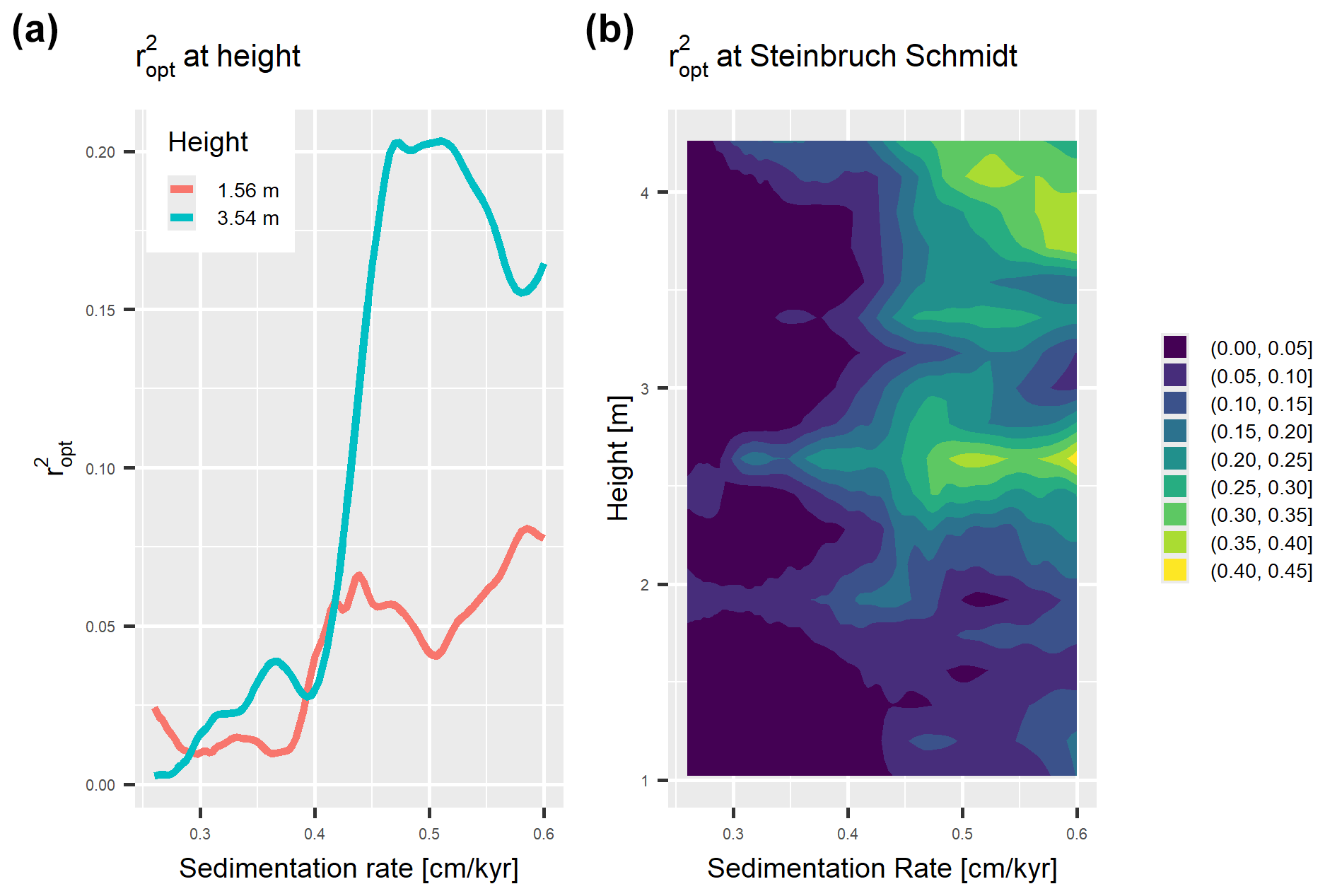
Figure 1 $r_{\mathrm{opt}}^{\mathrm{2}}$ values from eTimeOpt testing for precession amplitude modulation at 3.54 and 1.56 m (a) and throughout the whole section (b) in the Steinbruch Schmidt section. The heights shown in panel (a) roughly correspond to the locations of the Upper Kellwasser bed and the location of the dated ash bed.

Da Silva et al. (2020) analyzed magnetic susceptibility (MS), log Ti concentration, and δ¹³C values, with similar results for all three proxies. For this example, we focus solely on MS. Data preprocessing and eTimeOpt analysis was kept identical to da Silva (2024) for comparability; see Da Silva et al. (2020) for details. Here, we show the results of eTimeOpt testing for precession amplitude modulation. Results for short eccentricity amplitude modulation are similar and are shown in the Appendix (Figs. 3, A1, A2). eTimeOpt results for $r_{\mathrm{opt}}^{\mathrm{2}}$ were extracted using the get_data_from_eTimeOpt function of the admtools package. Interpreting eTimeOpt results probabilistically has two challenges:

1. At fixed heights, it provides $r_{\mathrm{opt}}^{\mathrm{2}}$ values as a function of sedimentation rate. However, it is unclear how $r_{\mathrm{opt}}^{\mathrm{2}}$ values can be meaningfully translated into a probability that the sedimentation rate falls within a certain interval.

2. The correlation structure of sedimentation rates is unclear. Given that we know sedimentation rates at one point in the section, how would that influence our estimates further up or down the section?

To address this, we introduce the following two assumptions into this example. Firstly, the sedimentation rates are determined at random heights following a Poisson process with rate λ, an assumption borrowed from BChron (Haslett and Parnell, 2008). This means the number of height points follows a Poisson distribution with an expected value of λ⋅l (where l is the length of the section) and that the locations of the points are independent and identically distributed according to a uniform distribution. Secondly, at each stratigraphic position, sedimentation rates follow a distribution with probability density function proportional to $r_{\mathrm{opt}}^{\mathrm{2}}$. As a result, sedimentation rates with a higher $r_{\mathrm{opt}}^{\mathrm{2}}$ are more probable than those with a low $r_{\mathrm{opt}}^{\mathrm{2}}$. If a range of sedimentation rates has comparable $r_{\mathrm{opt}}^{\mathrm{2}}$ values, they are all equally probable, alleviating the problem with eTimeOptTrack that only the sedimentation rate with the highest $r_{\mathrm{opt}}^{\mathrm{2}}$ is selected (Fig. 1). Thirdly, between the selected points, sedimentation rate changes linearly. These assumptions are incorporated by the sed_rate_from_matrix function, which takes the outputs of the get_data_from_eTimeOpt function and returns a sedimentation rate factory as required by ICON.

To illustrate the contributions of uncertainties introduced by the U–Pb date and those from eTimeOpt's estimated sedimentation rates, we decompose the construction of the age–depth model into two steps: firstly, an age–depth model measures time relative to the bentonite layer as the fixed single tie point with known age (Fig. 2a) and accounts only for the uncertainty resulting from the sedimentation rate is constructed; secondly, the age and uncertainty of the bentonite layer as determined by Percival et al. (2018) (372.36 ± 0.053 Ma (2σ), considering only measurement uncertainties) is added to the estimation procedure (Fig. 2b). For this example, we choose a rate parameter λ=3 for the sedimentation rate, use 1000 Monte Carlo samples to generate age–depth models, and report results rounded to the next kyr.

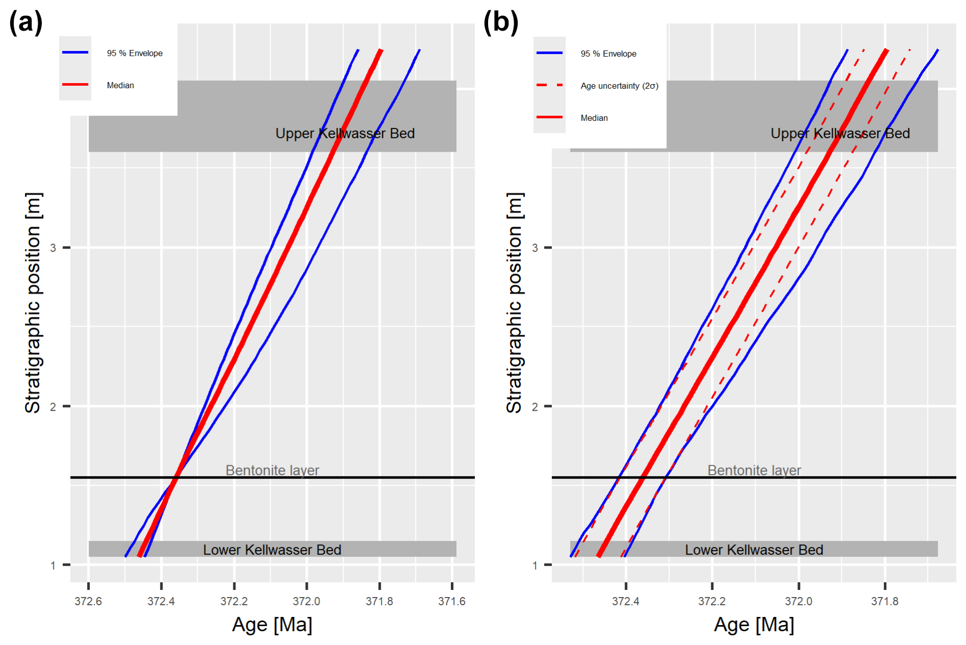
Figure 2 Age–depth models with (a) and without (b) incorporating the uncertainty of the radiometric dating for the Steinbruch Schmidt section based on eTimeOpt results testing for precession amplitude modulation. In panel (a), all uncertainties in the age–depth model arise from the uncertainties of the sedimentation rates estimated using eTimeOpt, while, in panel (b), they are a combination of the uncertainty of the radiometric dates from Percival et al. (2018) (dashed lines) and sedimentation rates estimated from eTimeOpt. Dashed lines in panel (b) indicate the age uncertainty of the section when the radiometric uncertainty is propagated using the median sedimentation rate.

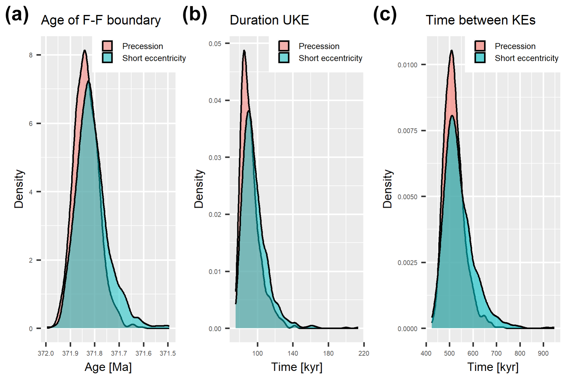
Figure 3 Durations of the Frasnian–Famennian boundary (a), Upper Kellwasser Event (b), and time elapsed between the Kellwasser events (c) based on testing for short eccentricity modulation and precession amplitude modulation.

3.1.1 Results

Both age–depth models show an increase in uncertainty away from the tie point due to variations in sedimentation rate (Fig. 2), resulting in the distinct sausage shape described by De Vleeschouwer and Parnell (2014). Median time contained in the 2.5 m between the bentonite layer and the Frasnian–Famennian boundary is 522 kyr with a 95 % highest density interval (HDI) of 159 kyr and a standard deviation (SD) of 39 kyr derived from the uncertainty of the sedimentation rate (Fig. 3). For the age–depth model incorporating the radiometric uncertainty, the 95 % envelope is almost parallel (Fig. 2b). This is because the uncertainties arising from the U–Pb date and the sedimentation rate estimates are independent and, as a result, sub-additive: it is unlikely that both simultaneously yield values that are too low (high), so their combined uncertainty is lower than the sum of their uncertainties. This indicates that, over the observed stratigraphically short interval, the error introduced by uncertainty in sedimentation rates is small relative to the uncertainty of absolute dates. Note that the uncertainty of sedimentation rates is limited by the maximum and minimum sedimentation rates passed to eTimeOpt and the averaging within the sliding window and therefore by the window size. In our case, the sedimentation rates were constrained a priori to the frequency distribution of sedimentation rates (piecewise for the windows used by eTimeOpt) derived from eTimeOpt based on its (the astrochron package's) $r_{\mathrm{opt}}^{\mathrm{2}}$ metric. This frequency distribution was obtained for the interval from 0.1 to 0.6 cm kyr⁻¹, as constrained by Da Silva et al. (2020). If a wider range of sedimentation rates were analyzed, sedimentation rates would contribute to more uncertainty in the age–depth model. The range is, in practice, constrained to reduce calculation time (Meyers, 2019). Running the eTimeOpt procedure for a broader range of sedimentation rates is possible, although more computationally intensive, but too broad a range may lead to false positives in terms of solutions with the best $r_{\mathrm{opt}}^{\mathrm{2}}$ values; therefore it is recommended to constrain the sedimentation rate using external knowledge, such as an independent chronometer or sedimentological information.

For the Frasnian–Famennian boundary, our age–depth model yields a median age of 371.837 Ma with a 95 % HDI of 201 kyr based on uncertainty from sedimentation rate and radiometric dates. The age distribution is approximately normal, resulting in an age estimate of 371.834 ± 0.101 Myr in the standard 2σ representation (Fig. 3). This is 36 kyr older than the age estimated by Da Silva et al. (2020), with age uncertainty reduced by 6 % (108 kyr vs. 101 kyr). Our uncertainty is lower than that listed by Da Silva et al. (2020), as they use multiple proxies, estimate one deterministic sedimentation rate per proxy, and combine these estimates to arrive at their final uncertainty. We use a single proxy (MS) to estimate uncertain sedimentation rates and propagate these uncertainties into the age estimate. Combining uncertain sedimentation rate estimates from multiple proxies would most likely give uncertainties comparable to or larger than 108 kyr, as adding sources of uncertainties can only increase the uncertainty of the final estimate. Becker et al. (2020) in Gradstein (2020) lists an age of 371.1 Myr ± 1.1 Myr (2σ) for the Frasnian–Famennian boundary. Both our mean age estimates and those of Da Silva et al. (2020) are elevated compared to this (by 734 and 770 kyr, respectively) but with reduced uncertainties (108 and 101 kyr, respectively) relative to the global geological timescale.

Mean duration of the Upper Kellwasser Event, stratigraphically expressed as black shale intervals, is 90 kyr (first and third quartile: 84 to 97 kyr; IQR: 13 kyr) and is positively skewed, matching the duration estimate of approx. 90 kyr by Da Silva et al. (2020). The median time elapsed between the Kellwasser events, measured from the top of the Lower Kellwasser Event to the bottom of the Upper Kellwasser Event, is 513 kyr (first and third quartile: 489 and 542 kyr; IQR: 54 kyr) and is also positively skewed (Fig. 3). Note that duration estimates are identical whether or not they are derived from age–depth models that incorporate radiometric uncertainty, and they depend solely on sedimentation rates. This is because the uncertainties of the tie point cancel out when calculating durations, allowing us to obtain duration estimates with uncertainties below those of the U–Pb dates by Percival et al. (2018). This shows that, even in the absence of absolute ages, information on sedimentation rates can be a powerful tool to determine durations and relative timing of events in deep time.

Neither the duration of the Lower Kellwasser Event nor the time from the onset of the Lower Kellwasser Event to the onset of the Upper Kellwasser event could be estimated with the applied approach. This is because the moving window approach in eTimeOpt does not provide sedimentation rate estimates for the lowest and highest parts of the section, of which the former contains the onset of the Lower Kellwasser Event. These durations could be estimated by using a narrower window in eTimeOpt; however, this would make the results not directly comparable to those of Da Silva et al. (2020).

Wichern et al. (2024) provide an estimated duration of the Lower Kellwasser Event of approx. 250 kyr at the nearby Winsenberg section. Combined with our estimates of 513 kyr between the end of the Lower Kellwasser Event and the onset of the Upper Kellwasser Event, the estimated time between the onset of both events is approximately 763 kyr, and the total duration of the Kellwasser crisis is approximately 852 kyr, slightly shorter than that estimated by Wichern et al. (2024).

3.2 Robustness of age–depth models for the Paleocene–Eocene Thermal Maximum

The Paleocene–Eocene Thermal Maximum (PETM) is a short interval of global carbon cycle perturbation associated with climate warming approximately 56 Myr ago (Vahlenkamp et al., 2020; Sluijs et al., 2007). Multiple causes have been proposed, including organic matter oxidation, enhanced volcanism, dissociation of gas hydrates, and methane release from vent systems (Dickens et al., 1995; Kurtz et al., 2003; Frieling et al., 2016; Storey et al., 2007). The PETM is a potential geological analog for anthropogenic climate change (Carmichael et al., 2017; Haywood et al., 2011), making it crucial to understand the timing of its onset and recovery.

Establishing the duration and timing of the PETM has been an important stimulus in improving age–depth modeling methods because of the changes in sedimentation rates affecting the stratigraphic tie points associated with the event. Many estimates rely on Ocean Drilling Program (ODP) sites from the South Atlantic and exploit combinations of cyclostratigraphy and extraterrestrial ³He flux coupled with characteristic changes in the δ¹³C record. The compilations of differences in timing of the PETM between studies by Sluijs et al. (2007) and Murphy et al. (2010b) are representative of the sensitivity of the age–depth models to their assumptions.

Here we attempt to replicate the analysis by Murphy et al. (2010b) based on IODP Site 1266 located at the Walvis Ridge. The core contains the entire PETM interval and has been among the key sections used to resolve the timing and pacing of the event. Murphy et al. (2010b) used measurements of extraterrestrial ³He coupled with the assumption of a constant extraterrestrial ³He flux into the sediment to estimate sedimentation rates and an age–depth model. Although the variability in ³He fluxes over geologically short timescales is low, it is known that the ³He flux can vary by about 1 order of magnitude over geologically long timescales (Takayanagi and Ozima, 1987; Farley, 2001; Sluijs et al., 2007). We use this study, firstly, to validate the FAM model and, secondly, to examine how robust the age–depth model for the PETM at Site 1266 from Murphy et al. (2010b) is to short-term variability in ³He fluxes.

As stratigraphic points of reference, we use the PETM core and recovery intervals as defined by Röhl et al. (2007), and we use the raw data published by Murphy et al. (2010a, b). We measure time relative to the beginning of the main interval to construct a floating age–depth model for the section, matching the timescale shown in Fig. 1 of Murphy et al. (2010b). While this does not give an absolute age of the PETM, it provides absolute durations of the PETM intervals defined above. For the constant flux value, we use the value of 0.48 pcc, where 1 pcc = 10⁻¹² cm³ of He at standard temperature and pressure (STP) per cm² per kyr, calculated by Murphy et al. (2010b). Note that the main text by Murphy et al. (2010b) gives a value of 0.37, but the calculations in their Table 1 and in their Supplement indicate that the value 0.48 had been used, and this is adopted here. We assume this value is a mean value, and the actual flux follows a normal distribution with this mean and a standard deviation of 0.04, reflecting the 2σ uncertainty of the flux estimate of 0.08 given by Murphy et al. (2010b). For the increase and decrease scenarios, we assume that, over an interval of 1 Myr, the flux values increase or decrease by a factor of 2. We use the base of the PETM, placed at the base of the clay, or “core”, interval at 306.78 mcd (m composite depth) as the base of the simulation and evaluate the age–depth model over the interval ranging upwards the core to 303.5 mcd, which is past the end of the recovery phase of PETM, placed at 304.19 mcd. We ran the analysis using 1000 Monte Carlo simulations and give results rounded to the next kyr.

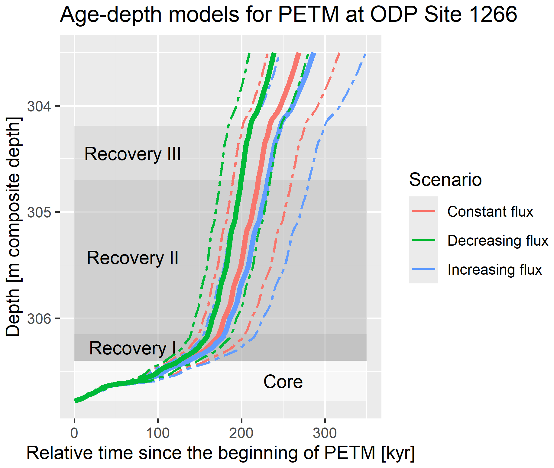
Figure 4 The three age–depth models for the PETM at IODP Site 1266 derived under the assumption of constant flux (red line), decreasing flux (green line), and increasing flux (blue line). Thick lines are the median age over 1000 replicates, and dashed lines are the 95 % envelope of the ages.

Figure 5 Density of the estimated duration of the PETM main and recovery interval.

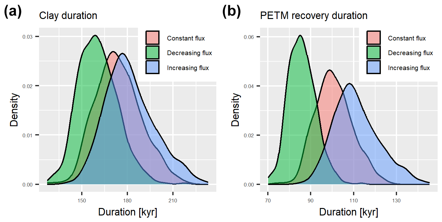
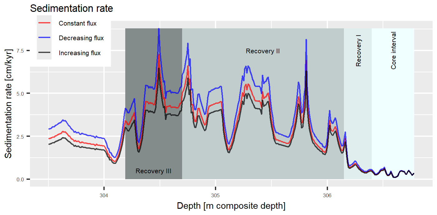
Figure 6 Median sedimentation rate in the stratigraphic domain for the three scenarios defined.

Figure 7 Median condensation in the stratigraphic domain for the three scenarios defined.

All three age–depth models show sedimentary condensation over the PETM core interval, expressed by the near-horizontal slope (Fig. 4). An increase in sedimentation rate is visible from the initial recovery interval (“Recovery I”) to the following intervals, Recovery II and Recovery III (Fig. 6). The median duration of the PETM (from the base of the clay interval to the end of the recovery) is 234 (2σ=39) kyr for the constant flux scenario and 212 (2σ=32) and 250 (2σ=45) kyr for the decreasing and increasing scenarios, respectively (Table 1). This duration is very close to the 234 ($+\mathrm{48}/\mathrm{-}\mathrm{34})$ kyr duration reported by Murphy et al. (2010b).

Table 1 Median durations of PETM phases at IODP Site 1266.

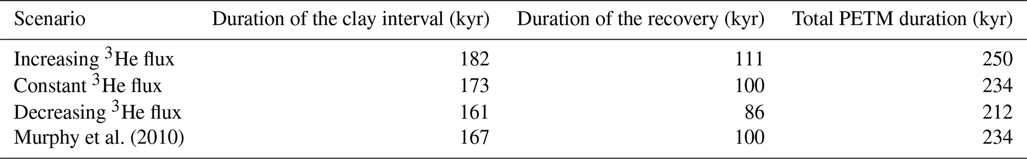
Median durations of the phases of PETM estimated under the three scenarios and their comparison with the results by Murphy et al. (2010b) are provided in Table 1. The disagreement between the results obtained using the FAM model and those reported in the original study does not exceed 6 kyr.

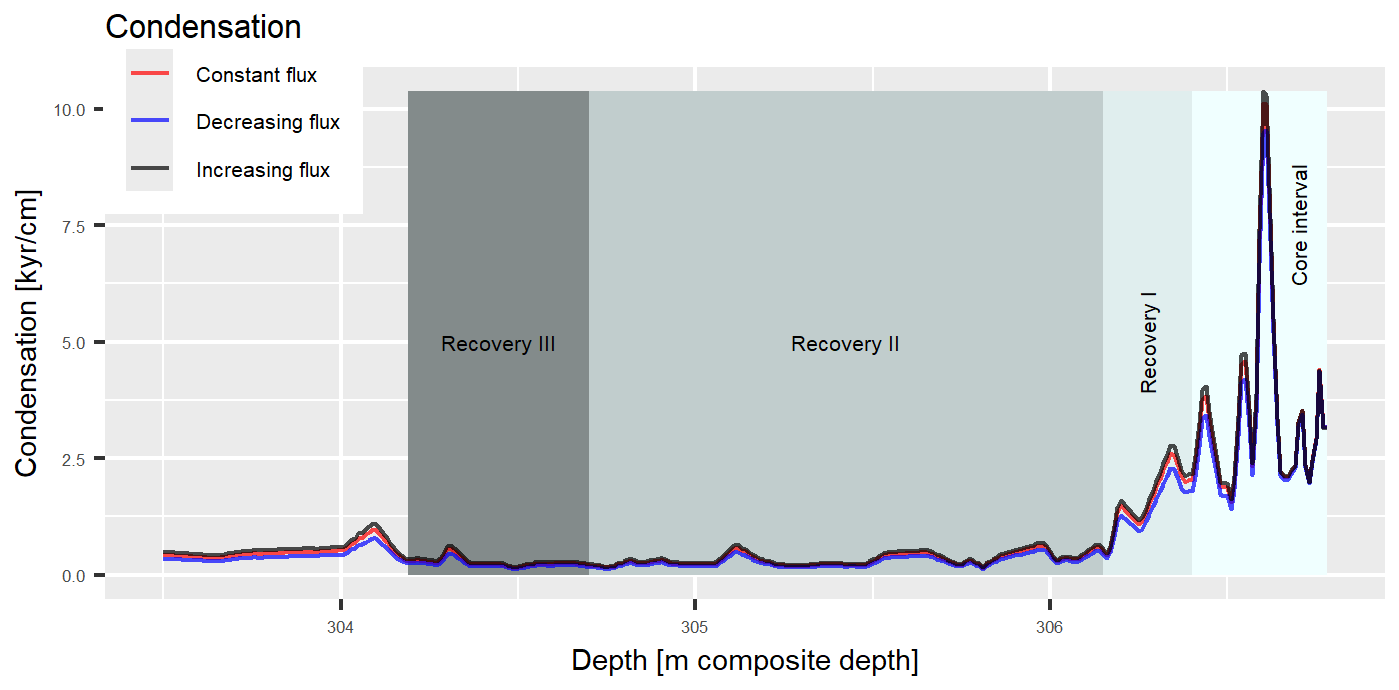
The PETM interval in the Site 1266 core spans 2.59 m. The age–depth model by Murphy et al. (2010b) relied on linear sedimentation rates calculated by combining constant ³He flux with a total duration of the interval derived from cyclostratigraphy (Röhl et al., 2007). Sedimentation rates have similar variability in all three scenarios. The range of sedimentation rates is 0.1 to 6.4 cm kyr⁻¹ for the increasing flux scenario, 0.1 to 7.3 cm kyr⁻¹ for the constant flux scenario, and 0.1 to 8.8 cm kyr⁻¹ for the decreasing flux scenario, with the lowest values at the transition of the pre-interval to the main interval and the highest values in the recovery interval (Fig. 6). Conversely, condensation ranges from 0.1 to 10.5 kyr cm⁻¹ across the scenarios (Fig. 7).

While there is no large offset in sedimentation rates and age–depth models between the scenarios, the varying fluxes generate systematic deviations from the constant flux scenario. Under increasing (decreasing) flux, sedimentation rates at the top of the examined interval are systematically lower (higher), leading to prolonged (shortened) durations of the recovery and clay intervals. Overall, results are consistent with those of Murphy et al. (2010b) and show that they are robust with respect to variations in ³He flux. Under decreasing flux, the median PETM duration differs by 10 % from the constant flux scenario (Table 1).

We conclude that variability in ³He fluxes by a factor of 2 on the timescale below 1 Myr has a moderate effect on the age–depth model at ODP Site 1266 and the derived estimates of PETM duration. Using tracer fluxes to estimate age–depth models is a powerful tool to estimate high-resolution age–depth models and identify local variations in condensation and sedimentation rates.

4 Discussion

We have introduced two methods to estimate age–depth models from complex stratigraphic or sedimentological data. ICON uses information on upsection change in sedimentation rate to estimate age–depth models, while FAM compares observed tracer values with assumptions on past tracer fluxes to constrain age–depth relationships. Informing a model with an external sedimentation or accumulation rate (whether a number or a distribution) is not conceptually different from informing it with tie points but presents a novelty of the ICON approach. This novelty may initially be a challenge for users, but it effectively presents an opportunity to enrich age–depth models with information previously not exploited: compilations of accumulation rates in depositional environments from actualistic studies (Sadler, 1981; Enos, 1991; McNeill, 2005; Scott, 2009), theoretical analyses on the temporal and spatial scaling of accumulation rates (Aadland et al., 2018; Tipper, 2016), and even relative estimates of sedimentation rates (Davies et al., 2019), equally handled by admtools. The novelty of this approach may initially result in seemingly higher uncertainty, but one should consider that it is in fact a quantification of uncertainty that had been present in all previous age–depth model inference but remained unaccounted for.

As examples of the use of ICON and FAM, we have applied the new methods to constrain the timing and duration of the Frasnian–Famennian boundary and the Upper Kellwasser Event with sedimentation rate constraints from cyclostratigraphy (Da Silva et al., 2020), and we have examined the robustness of age–depth models for the Paleocene–Eocene Thermal Maximum (PETM) to variations in tracer fluxes (Murphy et al., 2010b).

4.1 Comparison with other methods

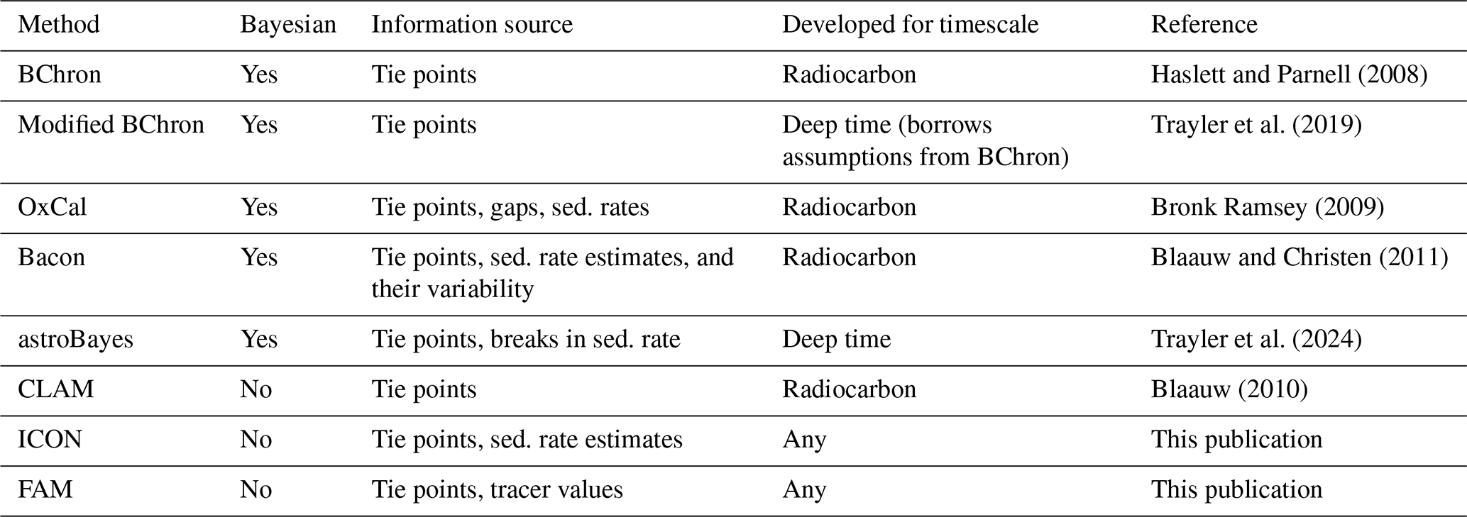
Bayesian approaches such as Bchron, modified Bchron, Bacon, and OxCal are common among the current methods to estimate age–depth models (Blaauw and Christen, 2011; Trayler et al., 2019; Haslett and Parnell, 2008) (Table 2). Trachsel and Telford (2017) pointed out that Bayesian approaches perform well compared to “classic” approaches such as CLAM. FAM and ICON are not Bayesian, as they do not rely on prior or posterior distributions. Bayesian methods can become computationally expensive when parameter spaces are high-dimensional. As stratigraphic data become more complex, the number of parameters and computation time increase. The computation time for the examples shown here is typically within minutes.

Haslett and Parnell (2008)Trayler et al. (2019)Bronk Ramsey (2009)Blaauw and Christen (2011)Trayler et al. (2024)Blaauw (2010)

Table 2 Comparison of different methods to estimate age–depth models.

By imposing monotonicity constraints on sample paths, Bayesian methods can resolve age reversals and reduce age uncertainties at the tie points. In ICON and FAM, users decide how to resolve age reversals, and the uncertainties of age–depth models at tie points cannot be improved upon by the method. In this hierarchical design, information from between tie points cannot reduce uncertainties of the tie points. Information on sedimentation rates and tracer fluxes is typically either expressed on an ordinal scale or associated with high uncertainty. The hierarchical design reflects the idea that an absolute age (e.g., from U–Pb dating) cannot be improved upon by information about the relative distribution of time (e.g., from changes in sedimentation rates) between tie points. Especially for changes in sedimentation rates estimated from cyclostratigraphy, this prevents circular reasoning, as the usage of external age constraints is recommended with cyclostratigraphic analysis (Sinnesael et al., 2019).

Assumptions on sediment accumulation employed by current methods to estimate age–depth models cannot possibly apply universally, since the dynamics of sedimentation vary between environments (Sadler, 1981). We do not know if sedimentary events follow a Poisson distribution across all timescales and depositional environments (e.g., Schumer and Jerolmack, 2009). It is not possible to prescribe upfront all correct combinations of assumptions for all possible use cases stratigraphers may study, also because the dynamics of sedimentation across timescales and environments remain themselves the topic of ongoing research (Aadland et al., 2018; Wilkinson, 2015; Davies et al., 2019), and age–depth models may feed back into this research by improving the inference on the structure of the geological record. ICON and FAM are an attempt to contribute to this research by making it possible to test different assumptions and validate them using stratigraphic and sedimentological information.

4.2 Limitations of this approach

In admtools v0.5.0 (Hohmann, 2025), neither ICON nor FAM can incorporate information on gaps in the stratigraphic record. Mathematically, it is possible to include gaps in ICON, and this will be implemented in later versions of the package. Similarly to constraining sedimentation rates, the inference of age–depth models may be constrained by the duration of gaps using literature information or calculations from average accumulation and sedimentation rates (Wilkinson, 2015; Paola et al., 2018; Tomašových et al., 2022). For FAM, incorporation of gaps is possible in the edge case of constant assumed tracer flux. For more complex assumed tracer fluxes, it is not obvious whether gaps can be incorporated, as they remove parts of the signal to which the observed tracer is matched. However, even with the option to incorporate hiatuses, hiatus durations and locations are notoriously challenging to estimate and justify empirically. Often times, the existence of hiatuses is invoked to explain a mismatch between signals of different sections. Hohmann et al. (2024) used forward simulations of carbonate platforms to show that gap duration and locations are functions of external drivers of stratigraphic architectures, and Meyers and Sageman (2004) used evolutive harmonic analysis to identify relatively short hiatuses (1–100 kyr) in a simulation study. These are just two examples showing that gap locations and durations are not random and that they can be identified with careful data analysis and forward models. Note that, in a case where there are unidentified gaps in a section, the reconstructed sedimentation rate will always be lower than the “true” sedimentation rate, leading to a Sadler-type effect (Sadler, 1981).

An assumption made by all methods to estimate age–depth relationships is that a given stratigraphic position has a unique age, which might be unknown but can be assigned an uncertainty. Dating of organic remains in modern environments (e.g., Dominguez et al., 2016 or Tomašových et al., 2018) shows that particle ages at a given location can differ significantly as a result of mixing in the surface mixed layer and thus violate this assumption. This effect might differ across environments, but time-averaging in Holocene deposits can reach values of multiple thousands of years (e.g., Berensmeier et al., 2023) and thus exceed the age uncertainty of age–depth models by several orders of magnitude. While Bayesian methods such as Bchron or Bacon automatically resolve reversals (Table 2), the maximum temporal resolution achievable in age–depth models will ultimately be limited by the depositional resolution of the sedimentary record, which is controlled by both physical (slumping, regularity of sediment supply) and biological (bioturbation) factors (Kowalewski and Bambach, 2008).

One key feature of FAM and ICON is that they are assumption-explicit in the sense that the user must specify all distributions that contribute to the age–depth model. While this requires additional coding effort, it results in an assumption-explicit age–depth model, where every assumption made is known and documented. As a result, uncertainties in age–depth models are a direct reflection of our understanding of the structure of the stratigraphic record. A second benefit is that age–depth model construction is replicable, even using different computational environments.

4.3 Uncertainties in age–depth modeling

For researchers using geohistorical data, age–depth models with low uncertainties are highly desirable. They allow the exact dating of events and provide low uncertainties of rates of past change, opening up the opportunity to use past climate perturbations as analogs for future climate change (Trayler et al., 2024). It is easy to construct an age–depth model with seemingly no uncertainties by simply connecting mean ages with a straight line (e.g., Tobin et al., 2012). However, low uncertainties should not be the target to assess the quality of age–depth models. Trachsel and Telford (2017) found that CLAM underestimates age uncertainties in varved sediments, and De Vleeschouwer and Parnell (2014) pointed out that, in the Devonian timescale in Gradstein (2012), age uncertainties decrease between absolutely dated tie points – an unexpected and counter-intuitive behavior. In the latter example, the problem could be corrected by applying the Bayesian Bchron approach (De Vleeschouwer and Parnell, 2014). Both examples demonstrate that there are empirical and logical lower bounds on uncertainties in age–depth models. In cyclostratigraphy, where this has been evaluated, even experienced users tend to overestimate the accuracy of age information calculated from age–depth models they build (Sinnesael et al., 2019). We argue that the best age–depth model should not be the one with the lowest uncertainty but the one that best reflects our understanding of and uncertainty about the structure of the stratigraphic record in the environment and timescale of interest. The importance of such contextual information was highlighted in the results of Cyclostratigraphy Intercomparison Project (CIP) (Sinnesael et al., 2019), which identified that cyclostratigraphic analyses lacking such context tended to be less accurate. However, contextual information and expert knowledge could not be – until now – consistently codified into the process of inferring an age–depth model. This poses an obstacle to replicability. Improving upon this situation poses a 2-fold challenge: firstly, understanding drivers of the local structure of the record; secondly, incorporating this information and the uncertainty associated with it into age–depth models. Currently, no standard for reporting uncertainty from different sources exists, although various approaches have been proposed (Zeeden et al., 2014; Huybers and Wunsch, 2004), but integrating uncertainties from biostratigraphy (Punyasena et al., 2012; Pálfy, 2007), range offset and biofacies (Holland and Patzkowsky, 1999), or sheer incompleteness (Hohmann et al., 2024) remains a technical challenge. CIP results led to the recommendation that age–depth models should be intercalibrated with other geochronometers (e.g., Jarochowska et al., 2020), but the question remains: what if two age–depth models for the same section, based on independent geochronometers, disagree? We propose that such alternative age–depth models can be treated as hypotheses in a hypothetico-deductive scientific framework and that stratigraphic data of interest can be evaluated under these hypotheses to assess how much stratigraphic uncertainty affects the conclusions of a study. However, admtools (Hohmann, 2025) allows one to add or remove information, leading to simple partitioning of uncertainty, as shown in example 1. For instance, the assumption of a constant flux of a tracer may be considered naive, especially over long timescales, and it is not always possible to validate it with independent data, as has been done by Middeldorp (1982) and Young et al. (1999). The assumptions of constant flux can nonetheless still be used as a null hypothesis, against which systematic or random changes in the flux can be tested.

When age–depth models are constructed with the widest breadth of stratigraphic and sedimentological information, timing and rates of past change might be associated with large uncertainties. However, these uncertainties will reflect our understanding of the structure of the stratigraphic record. On the other hand, incorporating information on the dynamics and internal rhythmicity of depositional environments, such as tidal or seasonal ones, in age–depth models provides us with new tie points and higher-resolution age–depth models. Both FAM and ICON turn complex information into age–depth models. To make full use of these methods, more research into this structure across environments, timescales, and external controls are required.

5 Conclusions

We have introduced two new methods, FAM and ICON, to estimate age–depth models from complex stratigraphic and sedimentological data. FAM compares observed tracer values with assumptions of fluxes in the time domain, while ICON uses information on changes in sedimentation rates (e.g., from cyclostratigraphy, sequence stratigraphy, or other expert knowledge) to construct age–depth models. Both methods are nonparametric in the sense that they do not make any a priori model assumptions other than that the law of superposition holds. Users can implement error models that reflect their knowledge about the local drivers of stratigraphic architectures, resulting in age–depth models that are data-driven and allow us to study uncertainty partitioning.

Appendix A: Additional figures

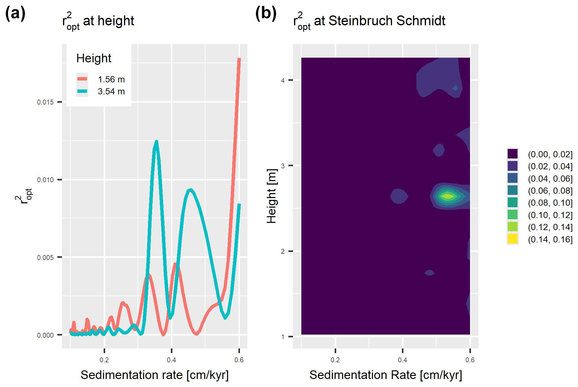
Figure A1 $r_{\mathrm{opt}}^{\mathrm{2}}$ values from eTimeOpt testing for short eccentricity amplitude modulation at 3.54 and 1.56 m (a) and throughout the whole section (b) in the Steinbruch Schmidt section. The heights shown in panel (a) roughly correspond to the locations of the Upper Kellwasser Bed and the location of the dated ash bed.

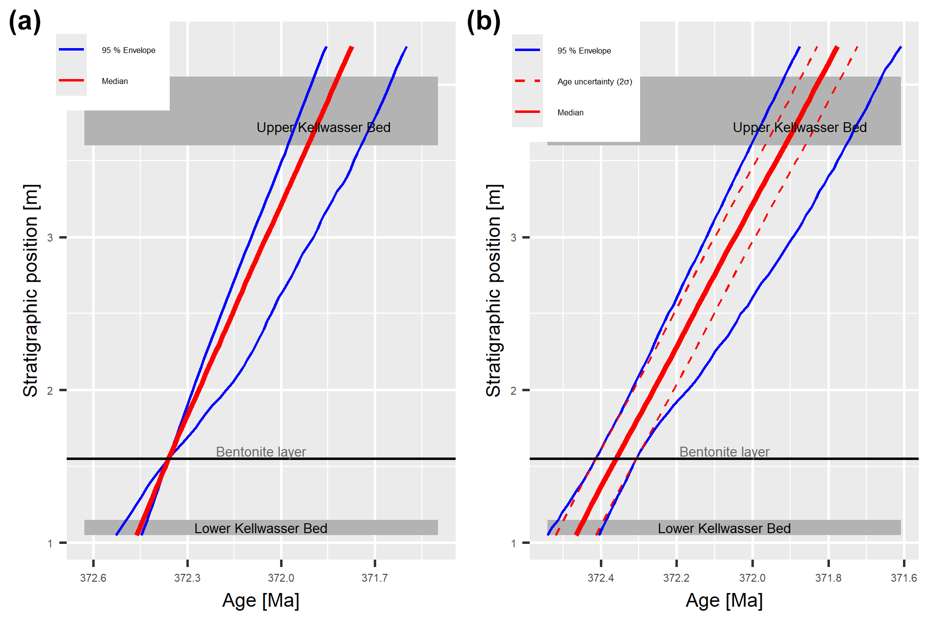
Figure A2 Age–depth models with (a) and without (b) incorporating the uncertainty of the radiometric dating for the Steinbruch Schmidt section based on testing eTimeOpt results for short eccentricity amplitude modulation. In panel (a), all uncertainties in the age–depth model arise from the uncertainties of the sedimentation rates estimated using eTimeOpt, while, in panel (b), they are a combination of the uncertainty of the radiometric dates from Percival et al. (2018) (dashed lines) and sedimentation rates estimated from eTimeOpt. Dashed lines in panel (b) indicate the age uncertainty of the section when the radiometric uncertainty is propagated using the median sedimentation rate.