Meteoric beryllium-10 fluxes from soil inventory measurements in the East River watershed, Colorado, USA

Meteoric beryllium-10 (¹⁰Be_met) has a wide range of applications as a geochronometer and tracer of geological processes. ¹⁰Be_met is produced in the atmosphere by cosmic rays and delivered to Earth's surface primarily via precipitation. ¹⁰Be_met is particularly suitable for quantifying surface process rates where use of in situ-produced ¹⁰Be is challenging, such as landscapes with quartz-poor bedrock. However, using ¹⁰Be_met for dating and quantifying surface process rates requires constraining depositional fluxes across space and time. Although empirical and physical models for predicting fluxes exist, the predictions can deviate substantially from measured values. Here we quantify ¹⁰Be_met flux in the East River watershed in Colorado, USA where precipitation is dominated by snowfall. We measured the ¹⁰Be_met inventory in soils on five glacial moraines 13–18 ka in age that span 700 m of elevation and calculated ¹⁰Be_met fluxes by dividing each inventory by moraine age. Inheritance-corrected fluxes range from 4.31×10⁵–1.80×10⁶ atoms cm⁻² yr⁻¹ and fluxes corrected using modeled erosional and desorption losses differ by a factor of 0.3 to 2.1. The predicted fluxes are well correlated with elevation, mean annual precipitation, mean snow depth, and snow water equivalent (R²=0.71 to 0.99). Regression models applied to gridded elevation, precipitation, snow depth, and snow water equivalent data predict watershed-averaged fluxes of 1.1×10⁶–3.8×10⁶ atoms cm⁻² yr⁻¹. Predicted fluxes from a published empirical model that estimates fluxes as a function of precipitation were 1.8–3.8 times higher than inheritance-corrected site fluxes, and 1.0 to 6.0 times higher than erosion- and desorption-corrected fluxes calculated using a profile-average desorption model. Fluxes predicted by general circulation models generally fall within the range of our empirically estimated watershed-averaged fluxes, although the degree of agreement depends on the predictor variable and whether inheritance-corrected or erosion- and desorption-corrected fluxes are used. Our results highlight both the importance of factors that drive variability in ¹⁰Be_met delivery to soils and how local calibration can improve estimates of ¹⁰Be_met flux in mountain watersheds.

1 Introduction

The cosmogenic nuclide beryllium-10 (¹⁰Be) is used widely for geochronology and to quantify rates of Earth surface processes (Brown, 1984; Bierman and Nichols, 2004; Willenbring and von Blanckenburg, 2010; Granger et al., 2013). ¹⁰Be forms during high energy collisions between cosmic particles and target nuclei (Lal and Peters, 1967). ¹⁰Be produced in Earth's atmosphere (typically from N and O) is known as atmospheric, garden variety, or meteoric ¹⁰Be (¹⁰Be_met), whereas in situ-produced ¹⁰Be (¹⁰Be_in situ) is formed in mineral lattices at and near Earth's surface. Production rates of ¹⁰Be_in situ are on the order of a few to tens of atoms g⁻¹ yr⁻¹ in quartz (Gosse and Phillips, 2001; Borchers et al., 2016). In contrast, ¹⁰Be_met is generated at orders of magnitude higher rates, with a global-averaged flux in excess of 1 million atoms cm⁻² yr⁻¹(Monaghan et al., 1986; McHargue and Damon, 1991). Prior to its deposition on Earth's surface by precipitation or dry fallout, ¹⁰Be_met resides in the stratosphere and troposphere for 2 years and 55 d, respectively (Yamagata et al., 2019). Hence global circulation transports ¹⁰Be_met from the site where it is produced in the atmosphere prior to its deposition (Field et al., 2006; Heikkilä et al., 2008). Once delivered to Earth's surface, ¹⁰Be_met adsorbs to and is co-precipitated on mineral surfaces, hence the highest concentrations are associated with secondary minerals and fine-grained particles with high surface areas (e.g., Graly et al., 2010). ¹⁰Be_met is partitioned with the solid phase at approximately neutral pH values (You et al., 1989). ¹⁰Be_met is thought to be retained in soils where pH is $>\sim \mathrm{4}$ (Graly et al., 2010), but laboratory experiments indicate pH 6 soils are more retentive than pH 4 soils and that retention also varies as a function of the type of organic compounds present (Boschi and Willenbring, 2016a, b). ¹⁰Be_met may be lost from upper soil horizons where low pH leads to leaching (Dixon et al., 2018), where clay minerals or humic material with adsorbed Be are translocated to greater depth (Pavich et al., 1984; Jagercikova et al., 2015), and where the surface of the soil has been eroded (Harden et al., 2002). Hence soil ¹⁰Be_met inventories depend on a variety of factors, including the local delivery rate, landform age, degree of chemical weathering, soil pH, and erosion rate (e.g., Graly et al., 2010; Willenbring and von Blanckenburg, 2010).

The high production rates, which allow ¹⁰Be${}_{\mathrm{met}}{/}^{\mathrm{9}}$Be ratios to be readily measured via accelerator mass spectrometry (AMS), the wide range of soils and regolith where ¹⁰Be_met is retained, and – unlike ¹⁰Be_in situ – the ability to be measured in non-quartz-bearing materials has allowed ¹⁰Be_met to be used widely as a geochronometer and tracer of Earth surface processes (e.g., Brown, 1987a, b; Graly et al., 2010; Willenbring and von Blanckenburg, 2010). For example, ¹⁰Be_met has been used to date terraces and moraines (Tsai et al., 2008; Egli et al., 2010; Dünforth et al., 2012), determine rock-to-soil production rates (Monaghan et al., 1992; McKean et al., 1993; Jungers et al., 2009), quantify soil residence times (Monaghan et al., 1983; Bacon et al., 2012; Foster et al., 2015), determine earthflow velocities (Mackey et al., 2009), trace sediment through hillslopes and fluvial systems (Brown et al., 1988; Reusser and Bierman, 2010; West et al., 2014; Campforts et al., 2016), and, when coupled with ⁹Be measurements, to quantify watershed-scale denudation rates and chemical weathering (von Blanckenburg et al., 2012; Wittmann et al., 2015; Dannhaus et al., 2018; Portenga et al., 2019; Deng et al., 2020b, 2021b). However, a requirement for using ¹⁰Be_met for dating and quantifying surface process rates is that the deposition rate or flux of ¹⁰Be_met (F_met, atoms cm⁻² yr⁻¹) to the study area is known.

Numerous efforts have been made to measure or predict F_met at local to global spatial scales and over annual to millennial timescales (Willenbring and von Blanckenburg, 2010; Graly et al., 2011). Direct measurement of ¹⁰Be_met concentrations in precipitation has been used to quantify ¹⁰Be_met flux at point scales and short timescales to develop empirical relations that predict F_met as a function of precipitation rate or latitude (Brown et al., 1989; Monaghan et al., 1986; Raisbeck et al., 1981; Graham et al., 2003; Graly et al., 2011; Willenbring and von Blanckenburg, 2010). Nuclide production functions (e.g., Lal and Peters, 1967; Masarik and Beer, 1999) are coupled with general circulation models (GCM) to simulate global scale spatial and temporal patterns of F_met as a function of geomagnetic field strength, solar activity, atmospheric circulation, and precipitation (Field et al., 2006; Heikkilä et al., 2008; Heikkilä and von Blanckenburg, 2015; Panovska et al., 2023; Zheng et al., 2021, 2024). Millennial-averaged values of F_met can be inferred from soils by measuring the ¹⁰Be_met inventory (I_met, atoms cm⁻²) and dividing the inventory by landform age (e.g., Egli et al., 2010; Reusser et al., 2010; Graly et al., 2011; Deng et al., 2021a).

However, there is often disagreement between F_met values determined from soil inventories, global-scale physical models, and precipitation-based empirical models (Ouimet et al., 2015; Deng et al., 2020a; Krone et al., 2024). Substantial variability in F_methas been documented at spatial scales smaller than the grid cell size (often several hundred km) of many GCMs (Ouimet et al., 2015; Clow et al., 2020; Deng et al., 2020a). The discrepancies and spatial variability likely stem from temporal and spatial fluctuations in ¹⁰Be_met production, atmospheric transport, and precipitation (Monaghan et al., 1986; Graham 2003; Jordan et al., 2003; Deng et al., 2020b; Krone et al., 2024). Hence, it is often desirable to locally-calibrate F_met prior to using ¹⁰Be_metto quantify surface process rates (e.g., Reusser et al., 2010; Ouimet et al., 2015; Deng et al., 2021a). Local-scale calibration is particularly important in mountainous settings, where microclimate variability can cause ¹⁰Be_met inventories and fluxes to vary over short distances (Ouimet et al., 2015). Here we quantify the ¹⁰Be_met flux at sites throughout the East River watershed, near Crested Butte, Colorado, USA (Fig. 1), a site of intensive research on the physical and biogeochemical drivers of watershed function (Hubbard et al., 2018). We measure ¹⁰Be_met inventories on independently dated glacial moraines, assess local-scale influences on ¹⁰Be_met flux, model potential losses of ¹⁰Be_met due to erosion and desorption, and compare ¹⁰Be_met flux measurements against predictions from empirical and physical models to evaluate the spatial variability and predictability of ¹⁰Be_met fluxes in alpine environments.

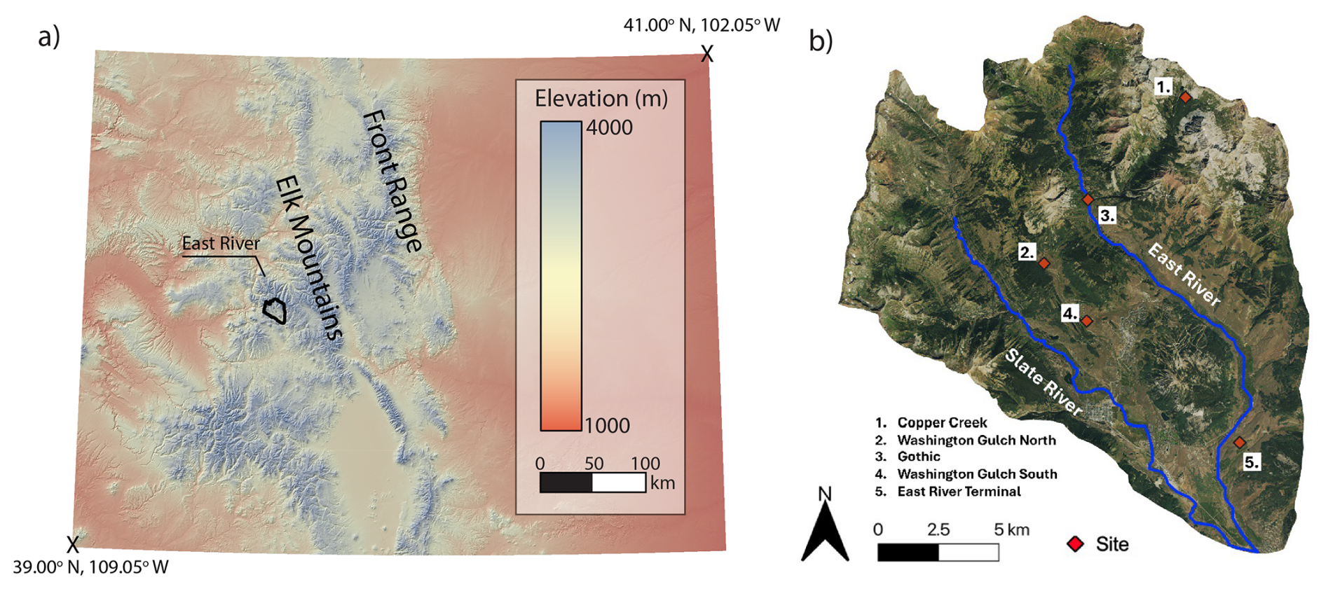
Figure 1 (a) Digital elevation model (DEM) of Colorado, USA showing the location of East River watershed. (b) Image of the East River watershed showing locations (red diamonds) where soil ¹⁰Be_met inventories were measured.

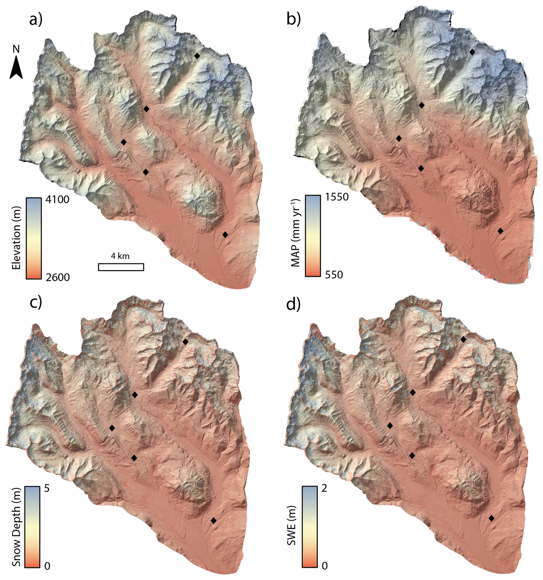
Figure 2 Maps of environmental variables within the East River watershed. (a) LiDAR-derived elevation data (Goulden et al., 2020); (b) downscaled Parameter-elevation Regressions on Independent Slopes Model (PRISM) mean annual precipitation (MAP) data averaged from 2008–2019 (Mital et al., 2022); (c) mean snow depth, and (d) mean snow water equivalent (SWE), derived from Airborne Snow Observatory data from 2018–2019 (Painter, 2018a, b). The black diamonds show each sample location.

2 Study Site

The East River drains the Elk Range of the Rocky Mountains in Colorado, USA (∼38.9° N, 106.9° W). The East River joins the Taylor River to form the Gunnison River, a major tributary to the Colorado River. The East River watershed and its tributaries, Washington Gulch and the Slate River, are a steep mountainous landscape, with elevations that range from 2600 to 4100 m above sea-level (Fig. 2a). The climate is characterized by long, cold winters and cool, short summers (Hubbard et al., 2018). The mean annual temperature is ∼0 °C, with mean minimum and maximum temperatures of −9.2 and 9.8 °C, respectively (Hubbard et al., 2018). Most of the annual precipitation occurs as snowfall, which can exceed several meters per year (Prather et al., 2023). Observations of enhanced precipitation rates on the windward side of mountains demonstrate that orography plays a strong role in controlling precipitation patterns within the watershed (Heflin et al., 2024). Hence like other mountain landscapes with orographically-influenced rain and snowfall (e.g., Roe, 2005), mean annual precipitation within the East River watershed increases with elevation (Fig. 2). The continental subarctic climate in the East River watershed supports montane, subalpine, and alpine ecosystems, which host aspen, meadow, mixed conifer, sagebrush, grass, sedge, and forb species (Fig. S1 in the Supplement) (Harte and Shaw, 1995). Bedrock in the watershed is primarily Cretaceous-age Mancos Shale and other sedimentary rocks that are intruded by Paleocene- to Miocene-age quartz monzonite porphyry and granodiorite rocks (Gaskill et al., 1967, 1991). Pleistocene glaciers eroded high elevation cirques and deposited moraines and outwash in the main East River valley (Gaskill et al., 1967, 1991). Exposure ages based on ¹⁰Be_in situ concentrations measured in samples from boulders indicate the terminal moraine at the end of the valley dates to 17.9 ka, whereas the youngest recessional moraine in a high-elevation cirque within the Copper Creek watershed was exposed at 13.0 ka (Quirk et al., 2024).

3 Methods

3.1 Field and laboratory methods

Soil ¹⁰Be_met inventories were determined for five glacial moraines with exposure ages that range from 17.9 to 13.0 ka (Fig. 1; Table 1; Quirk et al., 2024). Soil pits were dug on the flattest part of each moraine crest to minimize the potential of post-depositional erosion, with the exception of the Gothic moraine site, which was opportunistically located where the East River has laterally eroded a cutbank into the moraine, permitting deeper sampling. The pits were dug until shovel refusal, to depths between 60 and 145 cm. At the Washington Gulch North site, we sampled from a soil pit on a flat portion of the moraine, and collected a sample on the same moraine that was exposed by a recent landslide ∼375 m from the soil pit to assess inheritance in a deeper sample than we could access by digging. Bulk density was determined at each site by driving a 90.8 cm³ steel cylinder into the soil at depths corresponding to different horizons and weighing the dry soil (Table S1 in the Supplement). Samples were collected in either 5 or 10 cm depth increments by pressing a stainless-steel box, open at the top and front, into the face of the soil pit and scraping soil into the box. Samples were dried and sieved to separate <2 mm particles. We combined samples from adjacent depths to generate composite samples that encompassed depth intervals that range from 10 to 20 cm. Samples were combined by mixing splits of the <2 mm size fraction in proportion to the total mass of <2 mm particles in each sampling interval. The combined <2 mm fractions were powdered using a tungsten carbide shatter box. We measured soil pH in water and in 0.01 M CaCl₂ to assess ¹⁰Be_met retention. The measurements in water were made by mixing ∼5 g of powdered <2 mm grain-size material with 12 mL ultrapure water. The CaCl₂ pH measurements were made by mixing approximately 5 g of powdered <2 mm material with 25 mL of 0.01 M CaCl₂ to maintain a 1:5 soil to solution ratio (You et al., 1989). The pH values were measured with a Fisher Scientific accumet AE150 probe calibrated with multiple U.S. National Institute of Standards and Technology-traceable standards immediately prior to use (for more details, please see Table S2).

Table 1 Age, location, topographic attributes, and estimated surface lowering rates for the sites used to assess meteoric ¹⁰Be flux.

Sample locations were determined using a Bad Elf Flex GNSS with sub-meter precision. Slope and curvature values (Fig. S2) were generated using 3 m LiDAR DEM (Goulden et al., 2020). Curvature (m⁻¹) was derived by fitting a polynomial surface to a neighbourhood of 11 pixels using LSDtopotools (Mudd et al., 2014). Surface erosion rate ($\mathrm{d}z/\mathrm{d}t$) values were measured for the Gothic moraine site using an in situ-produced ¹⁰Be depth profile (Quirk et al., 2024) and modelled for the other sites using Eq. (4).

¹⁰Be_met chemistry was conducted at the University of Massachusetts Cosmogenic Nuclide Laboratory using the Stone (1998) fusion method. Approximately 0.5 g of homogenized and pulverized <2 mm soil particles was weighed into 30 mL Pt crucibles. We then added ∼350 µg of ⁹Be from a carrier with a ${}^{\mathrm{10}}\mathrm{Be}{/}^{\mathrm{9}}\mathrm{Be}$ ratio of $\sim \mathrm{1.75}\times {\mathrm{10}}^{-\mathrm{15}}$ to each sample. We also added 1000 µg of Al from a commercial carrier, which reportedly improves Be yields (Stone and Balco, 2004). Samples were dried overnight at 60 °C, then mixed with ∼2.5 g of KHF₂ and ∼0.5 g of Na₂SO₄ flux prior to heating with a gas torch to melt the sample. Once the samples were fully melted, they were heated for an additional 1–2 min. Be was extracted by soaking the crucibles with the fusion cakes overnight in 200 mL of ultrapure water. The solution was reduced to a volume of ∼30 mL by evaporation, then centrifuged. We decanted the supernatant and added ∼10–15 mL of 49 % HClO₄ to precipitate K as KClO₄. The solution was centrifuged to remove KClO₄ and the supernatant was dried overnight in Teflon beakers following addition of 1 mL of 8 M HNO₃. The samples were redissolved in 25 mL ultrapure water and Be was precipitated as BeOH by adding drops of ∼10 % NH₄OH until the solution pH was ∼9. The Be(OH)₂ was washed multiple times by repeatedly centrifuging, pouring off the supernatant, and remixing the Be(OH)₂ with ultrapure water. The Be(OH)₂ was dissolved with 2–3 drops of 6 M HCl, dried overnight in a quartz crucible, calcined by heating with a gas torch until BeO remained incandescent for 1 min, and packed into cathodes with Nb powder. The ${}^{\mathrm{10}}\mathrm{Be}{/}^{\mathrm{9}}\mathrm{Be}$ ratios were analyzed by AMS at Lawrence Livermore National Laboratory (LLNL) against AMS Be standard 01-5-4 (LLNL standard 07KNSTD) (Nishiizumi et al., 2007). ¹⁰Be concentrations in soil samples were blank-corrected by subtracting ${}^{\mathrm{10}}\mathrm{Be}{/}^{\mathrm{9}}\mathrm{Be}$ ratios measured in full process blanks from ratios measured in samples, with uncertainties added in quadrature.

Primary and secondary soil minerals contain ⁹Be at parts-per-million concentrations (e.g., Barg et al., 1997; Bacon et al., 2012). To assess the amount of naturally-occurring ⁹Be relative to the amount added as carrier, we dissolved ∼0.1 g of each sample in 49 % HF, reconstituted the samples in a 1 % HNO₃ + 1 % H₂SO₄ solution, centrifuged to separate insoluble organic matter, and measured Be in the supernatant via Inductively Coupled Plasma – Optical Emission Spectroscopy (ICP-OES).

3.2 ¹⁰Be_met inventory and flux analysis

We determined millennial-averaged F_met values for each moraine by measuring the ¹⁰Be_met inventory. The inventory was determined by multiplying the inheritance-corrected ¹⁰Be_met concentration (N_corr, atoms g⁻¹), by soil bulk density (ρ, g cm⁻³), the thickness of the sampling interval (z, cm), and the volumetric fraction of fine (<2 mm) soil V_f, and summing the values for all (n) individual sample depth increments (i) (e.g., Deng et al., 2021a):

$$\begin{array}{}\text{(1)}& I_{\mathrm{met}}=\sum _{i=\mathrm{1}}^n(N_{\mathrm{corr}}\cdot \mathit{\rho }\cdot z\cdot V_{\mathrm{f}}{)}_i.\end{array}$$

Using soil inventories to quantify F_met assumes that ¹⁰Be_met accumulation begins at the time a landform is initially exposed to wet and dry fallout. However, the ages of the moraines we use to constrain flux are orders of magnitude lower than the ¹⁰Be half-life (1.387 Ma; Chmeleff et al., 2010; Korschinek et al., 2010). Hence the soils we collected contain inherited ¹⁰Be_met atoms that were sorbed to mineral surfaces prior to their incorporation within the moraines. The inherited concentration was identified, following methods from prior work (e.g., Reusser et al., 2010), by the presence of a near constant ¹⁰Be_met concentration in the lower part of the depth profile. At four of the five sites, the ¹⁰Be_metconcentration reached a near-constant value with depth (Fig. 3). We assumed the concentration measured in the lowest depth interval was equal to the inherited ¹⁰Be_metconcentration and subtracted that value from concentrations measured in overlying samples (e.g., Reusser et al., 2010) and added the 1σ AMS analytical uncertainties in quadrature. If the ¹⁰Be_metconcentration in the sample used for the inheritance correction was greater than the concentration of a sample higher in the profile (e.g., at the Gothic moraine site), we set the concentration for that depth interval to zero. At the fifth site in the Copper Creek watershed, the ¹⁰Be_met profile is well-mixed above an indurated stone line at the base of the soil (Fig. 3a). Hence, we used the mean inheritance value of 7.58×10⁷ atoms g⁻¹ measured at the other four sites to correct for inheritance at the Copper Creek site.

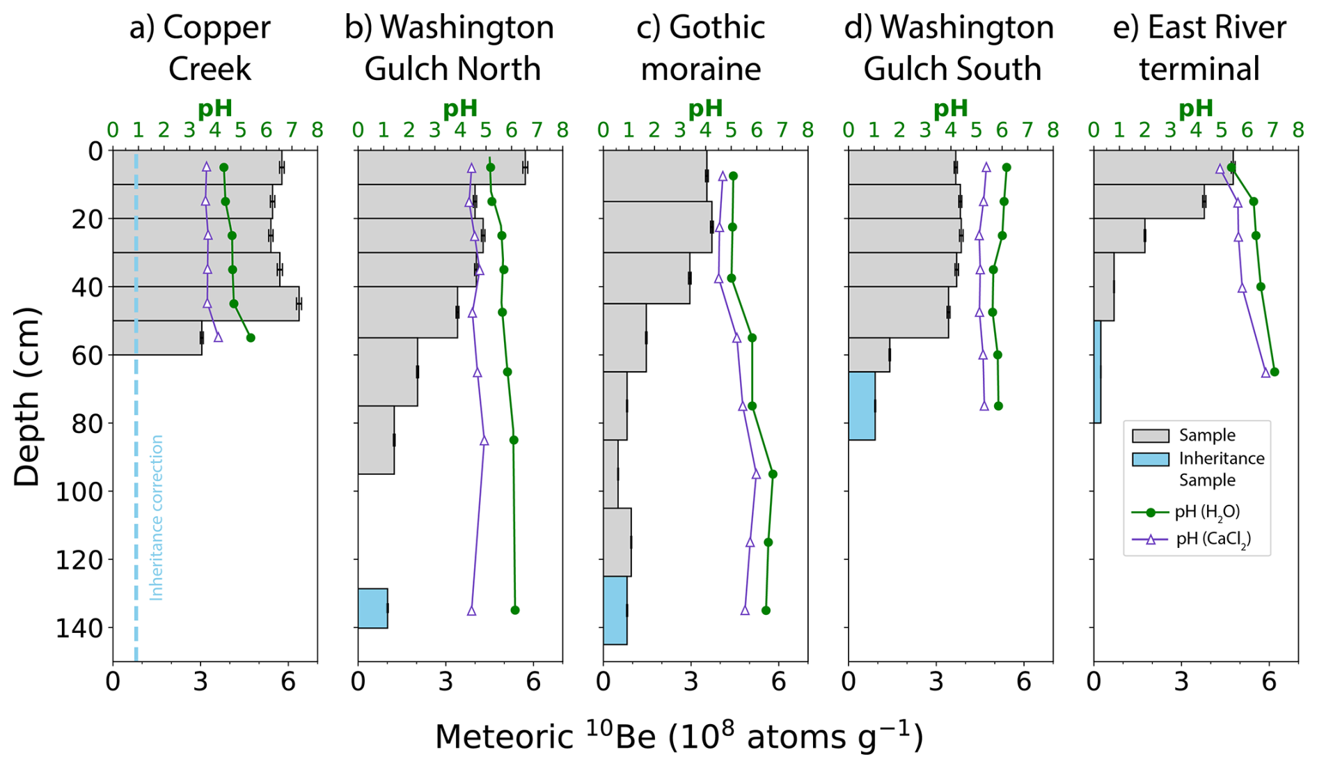
Figure 3 ¹⁰Be_metconcentration and pH as a function of depth for (a) Copper Creek, (b) Washington Gulch North, (c) Gothic, (d) Washington Gulch South, and (e) East River Terminal moraines. Grey boxes show measured concentrations and uncertainties. Blue boxes indicate samples assumed to represent the inherited ¹⁰Be_met concentration. In (a), the blue dashed line shows the mean inheritance value calculated from profiles (b)–(e). The sample used for the inheritance correction in (b) was sampled from a landslide exposure on the Washington Gulch North moraine that was 374 m away from the soil pit where the other samples were collected.

Since we measured bulk density by soil horizon, and not sample depth interval, we assigned bulk density values to each sample interval based on soil horizons identified in the field (Table S3). The volumetric fraction of <2 mm soil particles was calculated for each depth interval following Deng et al. (2021a) as: $V_{\mathrm{f}}=(\mathrm{1}-V_{\mathrm{c}\mathrm{1}})\times (\mathrm{1}-V_{\mathrm{c}\mathrm{2}})$, where V_c1 and V_c2 are volumes of two sizes of coarse clasts. V_c1 was determined by sieving each sample to separate <2 and >2 mm clasts and the volume fraction of >2 mm clasts was calculated assuming a density of 2.65 g cm⁻³. V_c2 was estimated by using field photos of each soil pit to digitize the area of large cobble- to boulder-sized clasts that were too large to be sampled by our 44.7 mm diameter steel ring. The volume fraction of large clasts was calculated by multiplying the area fraction by two-thirds (e.g., Deng et al., 2021a). We propagated uncertainty for individual depth increments by adding uncertainty associated with the inheritance-corrected ¹⁰Be_met concentrations and an assumed 5 % relative uncertainty in both ρ and V_f, in quadrature.

Given that the age of the moraines we sample is much less than the mean life of ¹⁰Be, and hence loss via decay is negligible, we divided the I_met value by moraine age (t, years) to determine the flux (e.g., Graly et al., 2010; Reusser et al., 2010; Ouimet et al., 2015; Clow et al., 2020; Deng et al., 2021a):

$$\begin{array}{}\text{(2)}& F_{\mathrm{met}}={\displaystyle \frac{I_{\mathrm{met}}}{t}}.\end{array}$$

Uncertainty in F_met for each calibration site was calculated by adding uncertainty in I_met values and moraine age in quadrature. Moraine age uncertainty was based on the standard error of the mean of multiple exposure ages on boulders or, for the Gothic moraine, a 1 ka uncertainty associated with a ¹⁰Be_in situ depth profile age (Table 1; Quirk et al., 2024).

The F_met values calculated using Eq. (2) assume complete retention of ¹⁰Be_met. We corrected fluxes (F_cor) for erosional and desorption losses according to Clow et al. (2020):

$$\begin{array}{}\text{(3)}& F_{\mathrm{cor}}=\left(\mathit{ϵ}\cdot N_{\mathrm{surface}}\right)+\left(I_{\mathrm{met}}\cdot \mathit{\lambda }\right)+\left(Q\times N_j/K_{\mathrm{d},j}\right),\end{array}$$

where ϵ is the erosion rate (g cm⁻² yr⁻¹), N_surface is the inheritance-corrected ¹⁰Be_met concentration in the uppermost sample that is assumed to represent the concentration in eroding soil (atoms g⁻¹), λ is the ¹⁰Be decay constant ($\mathrm{4.998}\times {\mathrm{10}}^{-\mathrm{7}}$ yr⁻¹), Q (L cm⁻² yr⁻¹) is the flux of water through the soil, and N_j and K_d,j are the inheritance-corrected ¹⁰Be_met concentration and Be partition coefficient (L kg⁻¹), respectively, for the soil depth interval j of interest, which is described below.

The ¹⁰Be_in situ depth profile method used to date the Gothic moraine, which was also sampled for ¹⁰Be_met, yielded a median $\mathrm{d}z/\mathrm{d}t$ value of $-\mathrm{2.3}\times {\mathrm{10}}^{-\mathrm{5}}$ m yr⁻¹ (Quirk et al., 2024). The source area for the Gothic moraine is primarily intrusive rock, hence the till matrix contained sufficient quartz for ¹⁰Be_in situ measurement. However, the till matrix was dominated by quartz-poor Mancos shale at the other sites and because of the dense shale-derived matrix, the pits could not be excavated deep enough to permit use of a ¹⁰Be_in situ profile to assess erosion rates. Hence we modeled the surface lowering rate at the other sites as:

$$\begin{array}{}\text{(4)}& {\displaystyle \frac{\mathrm{d}z}{\mathrm{d}t}}=D{\mathrm{\nabla }}^{\mathrm{2}}z,\end{array}$$

where D is the topographic diffusion coefficient (m² yr⁻¹), and ∇²z is topographic curvature (m⁻¹). Equation (4) is appropriate for low-gradient hillslopes like the moraines we sampled (Table 1), where surface lowering rates scale linearly with curvature (e.g., Kwang et al., 2022). Based on the median surface lowering rate and topographic curvature (Table 1), we infer the value of D at the Gothic moraine site is $\mathrm{5.8}\times {\mathrm{10}}^{-\mathrm{4}}$ m² yr⁻¹. Given the similar soils and climate, we assume D is comparable across the five moraines and use the diffusion coefficient for the Gothic moraine site and topographic curvature values to estimate $\mathrm{d}z/\mathrm{d}t$ values at the four sites that lack direct measurements. We assume $\mathrm{d}z/\mathrm{d}t$ values from Eq. (4) are equivalent to ϵ values in Eq. (3) and convert from units of length per time to mass per area per time using bulk density values inferred for the N_surface sample (Table S3).

We calculate Q as the difference between mean annual precipitation (MAP) and evapotranspiration (ET), which assumes that only the fraction of the precipitation that infiltrates the entire soil profile contributes to desorption losses. We determined MAP at each site using downscaled (400×400 m) Parameter-elevation Regressions on Independent Slopes Model (PRISM; Daly et al., 2008) raster data, which averages over the period from 2008–2019 (Mital et al., 2022). We used annual ET data from 2014–2015 that were simulated using the Community Land Model (CLM). ET values were reported for discrete locations within the East River watershed (Tran et al., 2019) and we assigned values to our study sites using the CLM prediction with an elevation and vegetation that most closely matched each site (Table S4). Following Deng et al. (2021a), we estimated K_d values using a logistic regression relationship from Campforts et al. (2016) where K_d is predicted as a function of pH measured in H₂O.

Prior work used Eq. (3) to assess ¹⁰Be_met desorption losses from the surface of the soil profile and assumed that desorbed Be exited the profile (Clow et al., 2020). Here we model three different desorption scenarios where N_j and K_d,j correspond to values for different depth intervals. The first analysis we conducted is for the soil surface sample, which yields results comparable to those of Clow et al. (2020). The second analysis uses profile-average values of N and K_d and assumes the mean K_d for the entire soil column is the primary influence on desorption losses. Because pH generally increases with depth, the third scenario uses K_d values for the lowermost sample in the profile and assumes desorption losses are controlled by the pH of the lowermost depth increment in the profile. The soil surface and lowermost sample scenario uses the respective K_d value and inheritance-corrected ¹⁰Be_met concentration associated with each depth interval for N_j. The profile-average scenario uses the weighted mean K_d value for the entire profile and the profile weighted mean value of the inheritance-corrected ¹⁰Be_met concentration for N_j, where the thickness of each sampling interval was used as the weighting factor. We report the results from all scenarios, but use the results of the profile-average scenario for regression analyses and for comparison against predictions from existing empirical and GCM-based models.

3.3 Relationships between flux, elevation, and precipitation

It is well-established that the flux of ¹⁰Be_met is strongly influenced by precipitation rates (e.g., Willenbring and von Blanckenburg, 2010; Graly et al., 2011). Given that precipitation within the East River watershed is orographically-controlled (Heflin et al., 2024), there should also be a relationship between elevation and the flux of ¹⁰Be_met. We used gridded datasets and univariate regression to assess the correlation between F_met (and F_cor) and elevation, MAP, snow depth, and snow water equivalent (SWE). The influence of elevation was evaluated using 3 m resolution LiDAR data (Goulden et al., 2020). We used the same gridded MAP data described in Sect. 3.2 that we use to estimate Q (Mital et al., 2022), and snow data products derived from the Airborne Snow Observatory (ASO; Painter et al., 2016). ASO combines airborne LiDAR and imaging spectrometry with snow energy balance models to generate spatial maps of snowpack properties. Snow depth is calculated as the difference between a snow-covered LiDAR survey and a snow-free “bare-earth” LiDAR scan. For this study, we used ASO-derived snow depth data (3 m resolution) acquired on 31 March 2018, and 7 April 2019 (Painter, 2018a). We used SWE data (50 m resolution) from the same dates as snow depth (Painter, 2018b). We used the coefficient of determination (R²) from linear regression analysis to assess the degree that variability in F_met and F_cor is explained by elevation and precipitation metrics. The significance of each regression model was determined using the associated p value. For the precipitation-based metrics, we additionally conducted regression through the origin analyses where the y-intercept was set to equal zero, because F_met and F_cor should be zero where precipitation is zero, assuming dry fallout of ¹⁰Be_met is negligible.

3.4 Comparing inventory-based fluxes against estimates from other methods

We predicted F_met for each of the five calibration sites using the precipitation- and latitude-based empirical model of Graly et al. (2011) using the down-scaled PRISM MAP data (Mital et al., 2022). We re-scaled the Graly et al. (2011) predictions, which are based on present-day precipitation measurements, to Holocene-averaged values by multiplying them by $\mathrm{1}/\mathrm{0.67}$ to account for differences in paleomagnetic and solar intensity variations (e.g., Clow et al., 2020) and compared the re-scaled predictions against our F_met and F_cor values.

The elevation, MAP, snow depth, and SWE data for each sample location were extracted from gridded datasets that span the entire watershed, including the Washington Gulch and Slate River tributaries. We applied the regression equations described in Sect. 3.3 to generate a prediction of flux for each pixel in the watershed. We then predicted watershed-average fluxes by calculating the mean value of all pixels. We used the regression through the origin models to generate predictions based on MAP, snow depth, and SWE to ensure model predictions were physically realistic (e.g., a negative y-intercept value could produce a negative flux value, which is physically-implausible). Our predicted watershed-average flux values integrate over a larger area, hence they are more appropriate for comparison against GCM-based flux estimates than our point-based values from each soil pit.

We compared our watershed-averaged flux predictions against three GCM-based predictions. The ECHAM5-HAM flux predictions of Heikkilä and von Blanckenburg (2015) are from a three-decade simulation that used pre-industrial aerosol and greenhouse gas concentrations and a modern solar modulation factor (φ) of 501.76 MeV. The solar modulation during the Holocene was lower (φ=280.94 MeV), hence Heikkilä and von Blanckenburg (2015) multiplied the fluxes by a factor of 1.23 to re-scale them to average Holocene values that represent the last 9400 years. The GEOS-Chem 14.1.1 and ECHAM6.3-HAM2.3 model predictions of Zheng et al. (2024) are modern predictions that average from 2005 to 2013 and use a φ value of 488 MeV. Since our flux estimates from the East River average over the Holocene, we multiply both of the Zheng et al. (2024) flux predictions by 1.23, which approximately re-scales them to Holocene-averaged values and makes them more comparable to our predicted watershed-average values.

4 Results

4.1 Soil pH

Soil pH for the uppermost sample interval of each profile ranged from 4.3–6.3 when measured in H₂O and from 3.7–5.4 when measured in CaCl₂ and the values generally increased with depth (Fig. 3; Table S2). Mean pH values averaged across all depths for Copper Creek, Washington Gulch North, Gothic, Washington Gulch South, and East River Terminal moraines are 4.7, 5.6, 5.7, 5.9, and 6.3, for measurements in H₂O, and 3.8, 4.6, 5.2, 5.2, and 5.8, when measured in CaCl₂, respectively. The most acidic soils are found at the Copper Creek site, which has the highest elevation and is dominated by spruce-fir forest vegetation (Fig. S1).

4.2 ¹⁰Be_metprofiles, inventories, fluxes, and controls on fluxes

AMS-measured ${}^{\mathrm{10}}\mathrm{Be}{/}^{\mathrm{9}}\mathrm{Be}$ ratios typically were on the order of $\mathrm{1.0}\times {\mathrm{10}}^{-\mathrm{12}}$ to $\mathrm{10}\times {\mathrm{10}}^{-\mathrm{12}}$, which is several orders of magnitude greater than the $\mathrm{2}\times {\mathrm{10}}^{-\mathrm{15}}$ to $\mathrm{5}\times {\mathrm{10}}^{-\mathrm{15}}$ ratios measured in blanks (Table 2). Measured ¹⁰Be_met concentrations ranged from about 2.4×10⁷ to 6.4×10⁸ atoms g⁻¹ (Table 2). Concentrations of ⁹Be were ∼1 ppm indicating the average mass of ⁹Be in the samples was ∼0.2 % of the mass added as carrier (Table S5). Given that 0.2 % is less than the uncertainty of the Be concentration of the carrier we used (1.2 %), no corrections were made to the AMS-measured ${}^{\mathrm{10}}\mathrm{Be}{/}^{\mathrm{9}}\mathrm{Be}$ ratios. The ¹⁰Be_met concentration profiles exhibit a variety of shapes. Profiles at four of the sites have relatively uniform concentrations in the upper ∼0.5 m of the profile, with maximum concentrations at or near the ground surface that decline at greater depths (Table 2; Fig. 3a–d). At the lowest elevation site on the terminal moraine, the ¹⁰Be_met concentration is greatest at the surface and declines exponentially with depth (Fig. 3e). The shallowest profile was at the Copper Creek site, where a coarse, indurated stone layer 60 cm below the ground surface prevented deeper sampling. At Copper Creek the concentration profile is well mixed in the upper 40 cm, exhibits a subsurface peak concentration 40–50 cm below the ground surface, and then declines sharply in the 10 cm interval directly above the stone line, but not to levels as low as those observed in the deepest samples from other profiles (Fig. 3a). Inheritance-corrected ¹⁰Be_met inventories range from 7.68×10⁹ to 2.35×10¹⁰ atoms cm⁻² (Table 3), with the largest and smallest inventories at the Copper Creek and East River terminal moraine sites, respectively. Inheritance-corrected F_met values range from 0.43×10⁶ to 1.80×10⁶ atoms cm⁻² yr⁻¹ (Table 3). Correcting for inheritance, erosion, desorption (using the profile averaged model), and decay yields F_cor values of 0.31×10⁶ to 3.7×10⁶ atoms cm⁻² yr⁻¹ (Table 4). Hence accounting for erosion and desorption caused fluxes to deviate from uncorrected values by a factor of 0.3 to 2.1 (Tables 3, 4). The desorption model scenarios for the uppermost and lowermost soil depth intervals predict fluxes that are generally within a factor of two of the profile-averaged model, except for the Copper Creek site, where the flux predicted from the upper sample pH is an order of magnitude greater than the flux predicted by the pH of the lowermost sample (Table 4).

F_met values are well-correlated with elevation and precipitation metrics in the East River watershed (Fig. 4; Table S6). F_met values are linearly correlated with elevation (R²=0.91), mean annual precipitation (R²=0.82–0.85), mean snow depth (R²=0.95–0.97), and mean SWE (R²=0.97–0.98). Due to the large range of elevation and precipitation within the watershed (Fig. 2), the regression models predict substantial within-watershed variability in F_met (Fig. 5). The erosion- and desorption-corrected fluxes based on the profile-averaged model exhibit similar trends with elevation and precipitation variables, but the correlations exhibited greater variability, with R² values of 0.96 for elevation, 0.56–0.95 for mean annual precipitation, 0.72–0.88 for mean snow depth in 2018–2019, and 0.66 to 0.90 for mean SWE in 2018–2019 (Fig. 4). The Copper Creek site has substantially higher elevation and precipitation values than the other sites and hence strongly influences regression relationships. When the Copper Creek site is omitted from the analysis, R² values range from 0.25 to 0.93 (Table S7).

Table 2 ¹⁰Be_met sample information and AMS results.

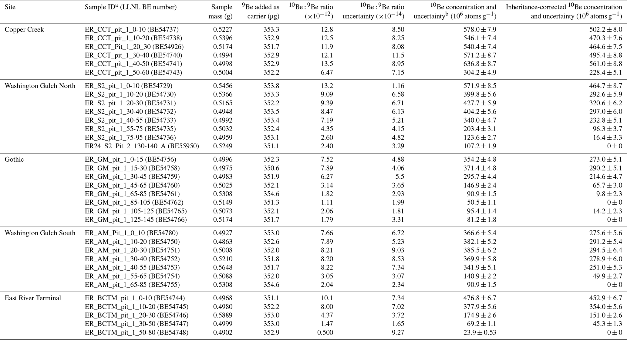
^a Values at the end of each sample ID refer to the sample depth interval (cm). ^b Reported ¹⁰Be concentrations are corrected using ${}^{\mathrm{10}}\mathrm{Be}{/}^{\mathrm{9}}\mathrm{Be}$ ratios measured in process blanks. ${}^{\mathrm{10}}\mathrm{Be}{/}^{\mathrm{9}}\mathrm{Be}$ ratios measured in process blanks in the same batches as the samples were: 2.44, 1.64, 2.55, 2.93, 2.11, 2.39, 4.71, 2.92, and $\mathrm{2.70}\times {\mathrm{10}}^{-\mathrm{15}}$. Uncertainty in I_met values was determined by adding the uncertainty for individual depth increments in quadrature. Analytical uncertainties were low (1.3 %–2.2 %) and the I_met uncertainties primarily reflect the uncertainties in ρ, V_f, and in some cases, the inheritance-corrected ¹⁰Be_met concentration. In some cases, uncertainties in the inheritance-corrected ¹⁰Be_met concentrations were large relative to the ¹⁰Be_met concentrations because the difference in concentrations between the two depth increments was small. Hence the Washington Gulch North and Gothic inventories have slightly higher uncertainties relative to the other sites.

Table 3 Environmental variable values and ¹⁰Be_met fluxes at each calibration site.

^a elevation (m) from Goulden et al. (2020), ^b mean annual precipitation (MAP) from Mital et al. (2022), ^c mean snow depth (m) from 2018–2019 (Painter, 2018a), and ^d Mean snow water equivalent (SWE) (m) from 2018–2019 (Painter, 2018b).

Table 4 Modeled erosional, decay, and desorption meteoric ¹⁰Be losses and loss-corrected fluxes.

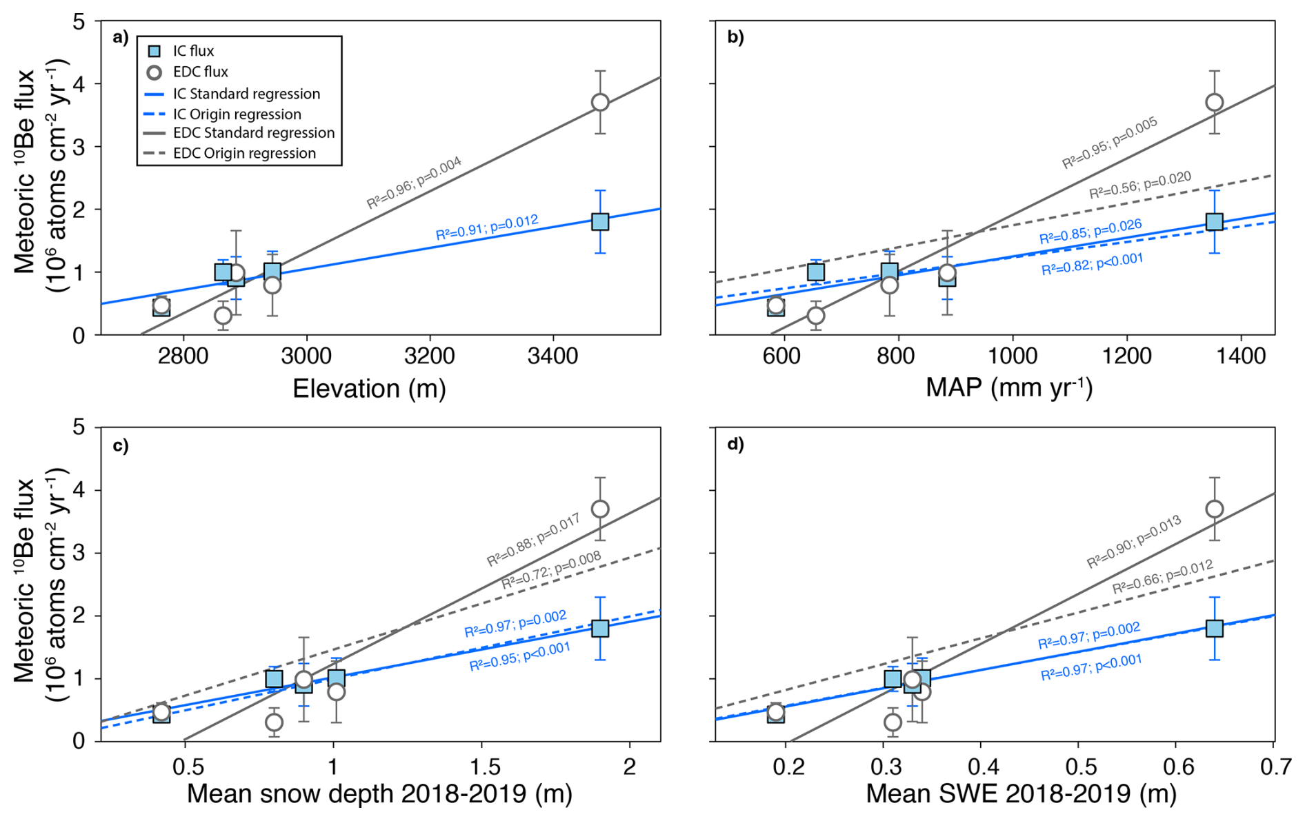
Figure 4 Linear regression models of ¹⁰Be_met flux versus (a) elevation, (b) mean annual precipitation (MAP), (c) mean snow depth (2018–2019), and (d) mean snow water equivalent (SWE) (2018–2019). Blue squares show inheritance-corrected fluxes and open gray circles show erosion- and desorption-corrected fluxes. The erosion- and desorption-corrected fluxes use the profile-average desorption model. For the inheritance-corrected (IC) data, solid blue lines show results from standard regression models and the dashed blue lines show regression through the origin models. For the corrected (EDC) data, solid grey lines show standard regression model results and grey dashed lines show regression through the origin models where the y-intercept is zero. Regression through the origin models are shown only for MAP, mean snow depth, and mean SWE. Regression coefficients, R² values, and p values are reported in Table S6. Figure S3 and Table S7 report regression results with Copper Creek excluded from the analysis. Figures S4 and S5 show the results from the uppermost and lowermost sample desorption models.

The different regression models predicted watershed-averaged F_met values that vary by about a factor of two (Table 5). For elevation, the regression models yield average F_met and F_cor of 1.30×10⁶ and 2.04×10⁶ atoms cm⁻² yr⁻¹, respectively. The MAP-based regression resulted in average F_met and F_cor values of 1.10×10⁶ and 1.48×10⁶ atoms cm⁻² yr⁻¹ for the standard and 1.11×10⁶ and 1.57×10⁶ atoms cm⁻² yr⁻¹ for the regression through the origin models, respectively. Snow depth models produced average F_met and F_cor values of 1.33×10⁶ and 2.07×10⁶ and 1.34×10⁶ and 1.97×10⁶ atoms cm⁻² yr⁻¹ for the standard and regression through the origin regression models, respectively. Similarly, SWE-based regressions yielded watershed-averaged F_met and F_cor values of 1.43×10⁶ and 2.34×10⁶ for the standard regression and 1.42×10⁶ and 2.05×10⁶ atoms cm⁻² yr⁻¹ for the regression through the origin models, respectively. We assessed the influence of extreme values and potential outliers by calculating watershed-averaged F_met and F_cor values using only pixels with the lowest 99th, 95th, and 90th percentile values, which resulted in lower mean values, with the greatest reductions for the snow-depth and SWE-based estimates (Table 5).

Table 5 Watershed-averaged ¹⁰Be_met flux predictions based on all pixels (100 %) and when excluding pixels with high values by using only the lowest 99th, 95th, and 90th percentile values when calculating the mean.

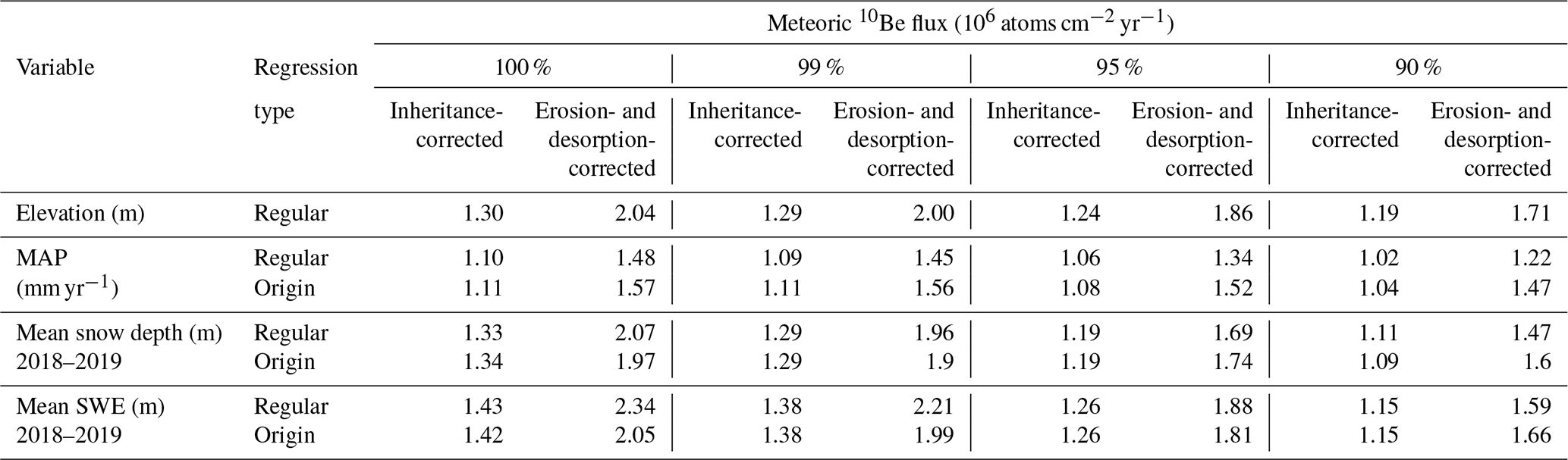
Values are calculated by applying regression equations to gridded elevation, mean annual precipitation (MAP), mean snow depth, and mean snow water equivalent (SWE) data to predict a value for each pixel in the watershed and then calculating the average of all pixels.

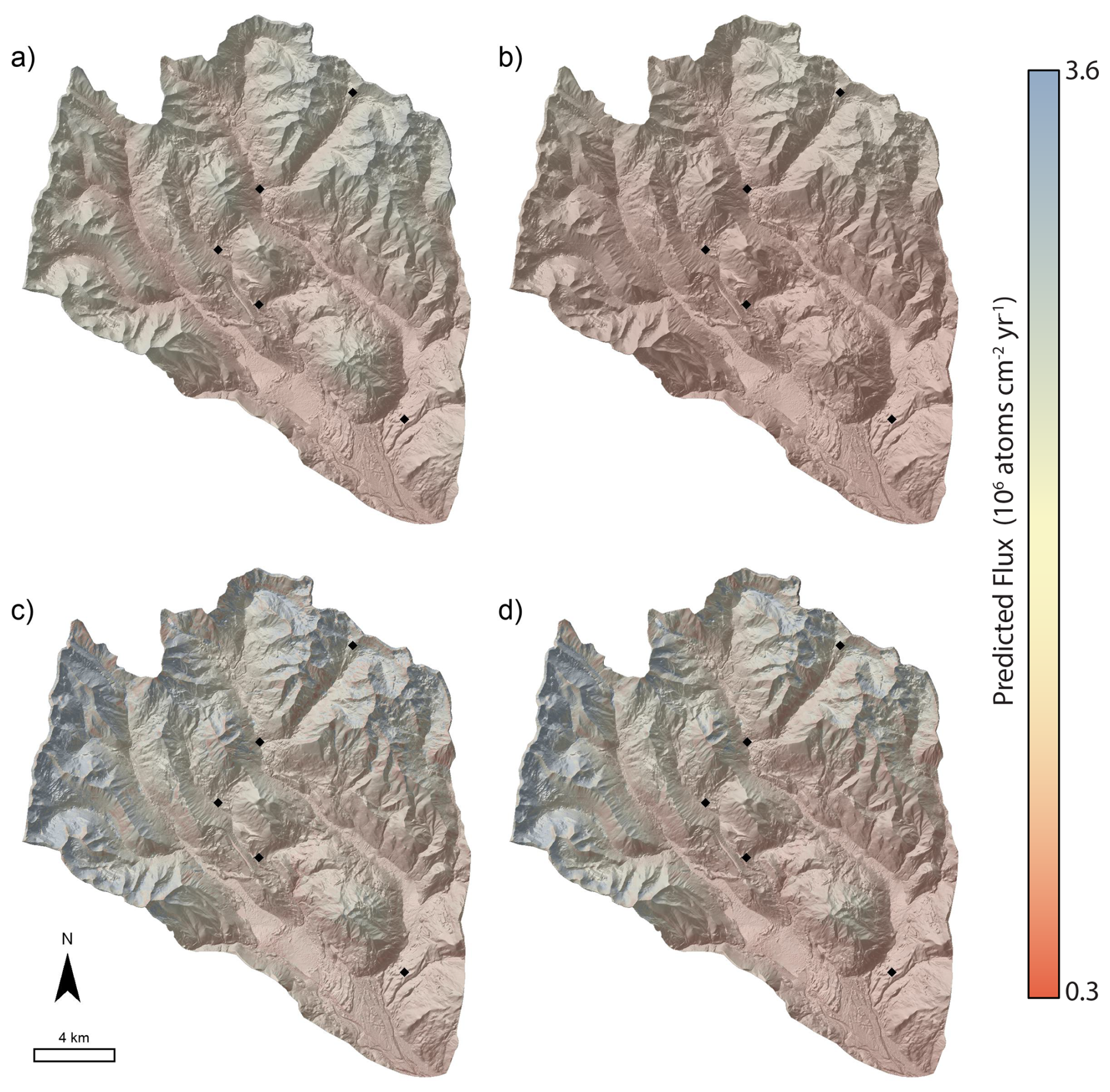
Figure 5 Spatial predictions of ¹⁰Be_met flux based on inheritance-corrected regression models using: (a) elevation with the regular regression; (b) mean annual precipitation with the origin regression; (c) mean snow depth from 2018–2019 with the origin regression; and (d) mean snow water equivalent from 2018–2019 with the origin regression. The equivalent results for erosion- and desorption-corrected fluxes calculated using the profile-average desorption model are shown in Fig. S6.

5 Discussion

¹⁰Be_met profiles tend to have characteristic shapes, and the shapes are sometimes used to infer processes of ¹⁰Be_met mobility (e.g., Graly et al., 2010). The two most common profile shapes are characterized by either a subsurface peak in concentration or concentrations that decline with depth from a maximum value at the soil surface (Graly et al., 2010). The profile on the East River terminal moraine exhibits an exponential decline in concentration with depth, however the concentrations at the other four sites are fairly uniform with depth. The uniform profiles likely arise from bioturbation, via vegetation or burrowing mammals. Pocket gophers (Thomomys talpoides) are the main soil-disturbing mammal within the East River watershed, and soil disturbance can be intense, with surveys indicating soil disturbance by burrowing can exceed one disturbance per m² within the elevation range of our sampling sites (Lynn et al., 2018). The distinct stone line at the Copper Creek site may have been generated by bioturbation (e.g., Johnson, 1989), though we cannot rule out the possibility of a periglacial origin (Ball, 1967). The stone line prevented deeper sampling at the Copper Creek site, which makes it difficult to determine whether the full ¹⁰Be_met inventory was sampled, or whether non-inherited ¹⁰Be_met is present below the stone line. In either case, the high-elevation Copper Creek site has the highest inventory, which is consistent with the higher precipitation rates at the site.

Glacial moraines erode via diffusive soil transport processes (e.g., Putkonen and Swanson, 2003) and loss of ¹⁰Be_met due to leaching has been documented or suspected in low pH soils with substantial chemical alteration (e.g., Pavich et al., 1984; Bacon et al., 2012; Dixon et al., 2018). The measured F_met values are hence minimum values because erosional and desorption losses of ¹⁰Be_met reduce inventories. Modeled erosional losses are largest at the Gothic moraine which has the most convex topography, whereas desorption losses are predicted to be greatest at Copper Creek where pH and therefore K_d are estimated to be lowest. The modelling predicts that desorption losses of ¹⁰Be_met predicted by the profile averaged model tend to be greater than erosional losses, particularly at the Copper Creek site, where predicted desorption losses are about an order of magnitude greater than desorption losses predicted for the other sites. In principle, accounting for erosional, decay, and desorption losses should increase flux estimates relative to the measured inheritance-corrected values. However, using Eq. (3) to account for erosion and desorption results in corrected fluxes that are similar to or less than the measured values for all sites except Copper Creek (Tables 3, 4), which suggests that the modeled loss terms may not fully capture true ¹⁰Be_met losses. Although the diffusion coefficient we calculate is comparable to values measured in other landscapes with similar climates (Richardson et al., 2019), there is still inherent uncertainty in using modeled, rather than measured, erosion rates and there is uncertainty in how rates of diffusive soil transport vary with elevation within the East River watershed. There is also uncertainty in the pH-derived K_d values, particularly because the presence of organic compounds, which are abundant in soil, alters sorption relative to experimental systems consisting of only mineral material (Boschi and Willenbring, 2016a, b).

F_met is highly correlated with elevation, MAP, snow depth, and SWE, which is unsurprising because these variables are related to one another via orographic controls on precipitation rates. However, different slope and intercept values for regression relationships result in different F_met and F_cor predictions for the same location and watershed-averaged fluxes that differ by a factor of about two. The precipitation data average over only a few decades and snow depth and SWE datasets cover only two winters, which are only small fractions of the post-glacial period over which ¹⁰Be_met has accumulated in soils. The recent snowfall magnitude may differ from Holocene averages, though the patterns are not likely to have varied substantially, given the orographic controls. However, unlike elevation and MAP datasets, the snow-based inventories yield insight on how local-scale topography may influence spatial patterns of F_met. For example, we predict that lower snow accumulation on sharp ridges relative to adjacent slopes leads to lower ¹⁰Be_met accumulation on ridges (Fig. 5). Watershed-averaged fluxes predicted using snow depth and SWE are more sensitive to extreme values than average fluxes based on elevation (Table 5). The mean snow depth of 1.90 m at the highest elevation Copper Creek site is a fraction of the highest snow depth values in the watershed, which exceed 20 m (Fig. S7) and indicates the highest snow depth values are potentially artefacts. The lack of F_met calibration sites in areas with higher snow accumulation may result in inaccurate predictions for such areas, however the lack of moraines or other stable, datable landforms at higher elevations makes it difficult to measure ¹⁰Be_met fluxes in such areas. The MAP data are based on decadal-scale precipitation measurements but are interpolated from weather station measurements using elevation as a predictor (Daly et al., 2008). However, the watershed-averaged MAP-based predictions are slightly lower than values based on elevation and snow data. Elevation is the only parameter not subject to temporal bias caused by measurement duration. Hence, given the orographic influences on precipitation within the watershed, elevation should be a robust predictor of ¹⁰Be_met fluxes. However, elevation-based predictions may be biased where local topography leads to persistent snow redistribution via wind and avalanches. Given the different ¹⁰Be_met flux predictions from the elevation, MAP, snow depth, and SWE datasets, an ensemble approach may be appropriate for using ¹⁰Be_met values to quantify surface process rates, in a manner similar to assessing results from multiple production rate scaling models when determining ¹⁰Be_in situ exposure ages (e.g., Balco et al., 2008).

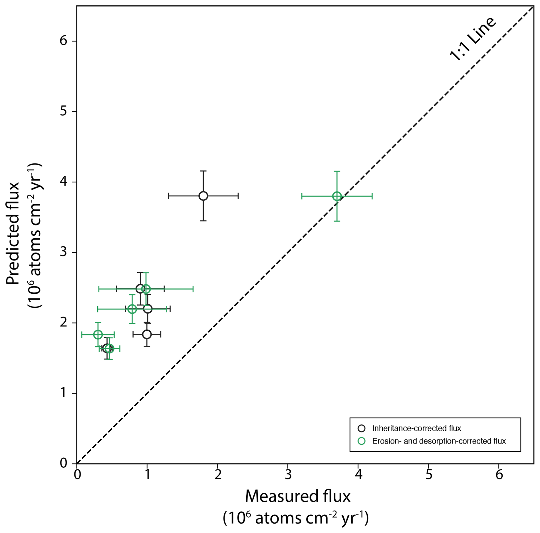
Figure 6 Predicted ¹⁰Be_met flux from the empirical precipitation-based model of Graly et al. (2011), scaled to reflect Holocene-average values (e.g., Clow et al., 2020) versus measured flux values for the five study sites. Measured erosion- and desorption-corrected fluxes use the profile-average desorption model.

Fluxes predicted by an empirical precipitation- and latitude-based model (Graly et al., 2011) are 1.8–3.8 times higher than measured inheritance-corrected fluxes (Fig. 6). The predicted fluxes are 1.0 to 6.0 times higher than the observed erosion- and desorption-corrected values. The empirical formulation of Graly et al. (2011) predicts fluxes as a function of both latitude and precipitation rate. Since our sites have essentially the same latitude, the variability in the predicted fluxes solely represents differences in precipitation. Hence the cause of the discrepancy in measured and predicted fluxes may simply reflect a different proportionality between precipitation and flux in the Graly et al. (2011) dataset, which included a worldwide compilation of sites, and the East River dataset. GCM-based models predict ¹⁰Be_met fluxes of 1.46×10⁶ atoms cm⁻² yr⁻¹ (Heikkilä and von Blanckenburg, 2015), 1.63×10⁶ atoms cm⁻² yr⁻¹(Zheng et al., 2024, ECHAM6.3-HAM2.3), and 2.12×10⁶ atoms cm⁻² yr⁻¹ (Zheng et al., 2024, GEOS-Chem 14.1.1) for the East River watershed and its tributaries (Fig. 7). A single grid-cell from the GCM-models covers an area larger than the watershed, hence the models simulate the influence of meso-scale atmospheric dynamics on ¹⁰Be_met flux, but do not capture within-watershed ¹⁰Be_met variability caused by orographic precipitation. For example, the highest GCM-based flux prediction is 7–13 times greater than the lowest erosion and desorption-corrected flux inferred for the Washington Gulch South site, but our watershed-average predictions only differ from GCM-based predictions by a factor of 1.0 to 1.9. In general, the watershed-averaged predictions from the measured, inheritance-corrected inventories better match GCM-based fluxes than watershed average fluxes corrected for erosion and desorption, which tend to be higher (Fig. 7). An exception is the MAP-based watershed-average flux (1.10–1.57×10⁶ atoms cm⁻² yr⁻¹), which is lower than predictions based on elevation (1.30–2.04×10⁶ atoms cm⁻² yr⁻¹), snow depth (1.33–2.07×10⁶ atoms cm⁻² yr⁻¹), and SWE (1.43–2.34×10⁶ atoms cm⁻² yr⁻¹), which causes the erosion- and desorption-corrected fluxes to better align with the GCM-based predictions (Fig. 7). Hence, the GCM-based predictions generally fall within the range of our empirically estimated watershed-averaged flux values, although the degree of agreement depends on the predictor variable and whether or not fluxes are corrected for erosion and desorption.

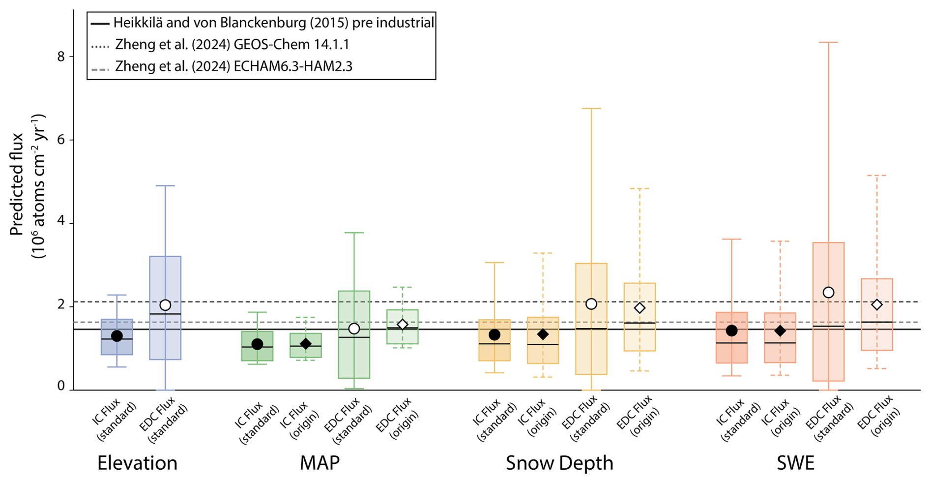
Figure 7 Watershed-scale ¹⁰Be_met fluxes predicted by empirical models based on elevation, mean annual precipitation (MAP), mean snow depth, and mean snow water equivalent (SWE) and flux predictions from global circulation-based (GCM) models. Boxplots show the median (horizontal line), interquartile range, and 5th and 95th percentiles of flux values. Mean fluxes are shown with circles (standard regression models, left box) and diamonds (regression through origin models, right box). GCM-based flux predictions from Heikkilä and von Blanckenburg (2015) and Zheng et al. (2024) are shown as horizontal lines. IC indicates inheritance-corrected fluxes and EDC indicates erosion- and desorption-corrected fluxes calculated using the profile-average desorption model.

Soils contain ¹⁰Be_metscavenged from the atmosphere by aerosols, but also from dust particles that are derived from aeolian erosion and transported in the atmosphere before being deposited (Monaghan et al., 1986; Graly et al., 2011). The dust-derived or “recycled” ¹⁰Be_met can be as much as ∼20 % of the total flux (Monaghan et al., 1986; Graham et al., 2003). Although the dust contribution to flux estimates does not need to be independently known to quantify surface process rates, provided that time-averaged delivery of dust to soils is representative of the timescale relevant to the surface process rate under investigation, dust contributions should be accounted for before comparing measured fluxes against predictions from GCMs. Hence the comparison of measured ¹⁰Be_met fluxes against the GCM-based predictions is somewhat complicated by the likely contribution of dust to our measured values. The contribution of dust to ¹⁰Be_met inventories in the East River is unconstrained. Contemporary dust fluxes of 5–10 g m⁻² yr⁻¹ have been measured in the San Juan Mountains of Colorado (Lawrence et al., 2010), but recent dust deposition is much greater than average Holocene values (Neff et al., 2008). Long term dust fluxes in the Colorado Front Range are low (Dethier et al., 2012) and dust is thought to contribute <10 % of the total flux of ¹⁰Be_met (Ouimet et al., 2015). If the contribution of dust in the East River is comparable to that in the Front Range, accounting for dust would not substantially influence the magnitude of discrepancies between GCM-based predictions and our empirically derived ¹⁰Be_met flux estimates.

At a regional level, ¹⁰Be_met fluxes for the Colorado Front Range based on soil inventories have been estimated to be $\mathrm{1.5}\pm \mathrm{0.2}\times {\mathrm{10}}^{\mathrm{6}}$ atoms cm⁻² yr⁻¹ (Ouimet et al., 2015). Soil inventory-based ¹⁰Be_met fluxes in the Wind River Mountains, Wyoming are $\mathrm{1.46}\pm \mathrm{0.20}\times {\mathrm{10}}^{\mathrm{6}}$ and $\mathrm{1.30}\pm \mathrm{0.48}\times {\mathrm{10}}^{\mathrm{6}}$ atoms cm⁻² yr⁻¹ for Pinedale- and Bull Lake-aged moraines, respectively (Clow et al., 2020). The 0.43–1.8×10⁶ atoms cm⁻² yr⁻¹ F_met values and 0.31–3.70×10⁶ atoms cm⁻² yr⁻¹ F_cor values we measure are consistent with those from the Front Range and Wind River Mountains, though those sites are drier, with ∼500 mm yr⁻¹ of mean annual precipitation in the Front Range (Ouimet et al., 2015) and 276 mm yr⁻¹ at the Wind River Mountains sites (Clow et al., 2020), relative to the 585 to 1353 mm yr⁻¹ precipitation at the five East River study sites. The driest site in the East River (terminal moraine, 585 mm yr⁻¹ MAP) has F_met and F_cor values of 0.43×10⁶ and 0.47×10⁶ atoms cm⁻² yr⁻¹, respectively, which are lower than fluxes inferred in the Front Range and Wind River Mountains. These comparisons suggest that precipitation contributes to regional differences in ¹⁰Be_met flux, but does not explain all of the variability among sites.

Local calibration of ¹⁰Be_met flux greatly increases the utility of ¹⁰Be_met as a tracer of surface processes in the East River watershed, where there is prevalent shale bedrock that is not very amenable to the more common ¹⁰Be_in situ method. Our findings show that, whereas ¹⁰Be_met flux predictions from GCM-based models are broadly applicable for large-scale watershed applications, such models do not capture the high spatial variability in ¹⁰Be_met fluxes that is driven by orographic influences on precipitation. Hence using ¹⁰Be_met to quantify physical erosion and weathering rates at the small watershed or soil profile-scale requires not only local-scale calibration of ¹⁰Be_met fluxes, but also a means for predicting ¹⁰Be_met fluxes for sites where elevation and precipitation are different from that of the sites used for calibration. Our study demonstrates how high-resolution LiDAR elevation and snowpack datasets can be combined with locally calibrated ¹⁰Be_met flux measurements to generate spatially resolved flux predictions, which furthers our understanding of the processes that control the delivery of ¹⁰Be_met to soils.

6 Conclusions

Meteoric ¹⁰Be fluxes calculated from soil inventories on five glacial moraines dated to 13.0–17.9 ka in the East River watershed, Colorado, USA range from 0.43–1.8×10⁶ atoms cm⁻² yr⁻¹ when corrected for inheritance only and 0.31–3.70×10⁶ atoms cm⁻² yr⁻¹ after also taking loss of ¹⁰Be by erosion and desorption into account. Accounting for pH-dependent desorption substantially increases the estimated flux at the Copper Creek site where soil pH is lowest. The inheritance-corrected and erosion- and desorption-corrected fluxes vary systematically with environmental gradients across the watershed and are generally correlated with elevation, mean annual precipitation, snow depth, and snow water equivalent, reflecting the important role orographic precipitation plays in influencing spatial patterns of meteoric ¹⁰Be flux within the watershed. Elevation is the only predictor of flux that is not subject to temporal bias, whereas the snow-based predictions are based on only two years of measurements, and the magnitude and pattern of snow accumulation during those years may vary substantially from Holocene averages. However, the snow-based predictions yield insight into smaller-scale topographic controls on meteoric ¹⁰Be fluxes, such as predictions of lower fluxes on sharp ridge crests relative to adjacent hillslopes due to snow redistribution. The fluxes measured at the five moraines are lower by a factor of 1.0 to 6.0 than predictions from an empirical model relating flux and mean annual precipitation and latitude (Graly et al., 2011). Watershed-averaged fluxes predicted from empirical correlations between measured flux and elevation, mean annual precipitation, mean snow depth, and mean snow water equivalent are comparable to predictions from global-scale GCMs. Although the GCM models do not capture the spatial variation in flux within the watershed and are of less utility for soil profile-based applications, the GCM results provide useful estimates of watershed-scale flux. The findings highlight the large degree which meteoric ¹⁰Be fluxes vary within alpine landscapes and demonstrate how combining soil meteoric ¹⁰Be inventories and high-resolution gridded datasets can generate spatially-resolved meteoric ¹⁰Be flux predictions. Our results enhance the utility of meteoric ¹⁰Be as a tracer of surface processes in the East River watershed, and other alpine landscapes with rocks that are not conducive to using in situ-produced ¹⁰Be and add to our overall understanding of the factors that influence the delivery and retention of meteoric ¹⁰Be in soils.