Robust isochron calculation

The standard classical statistics approach to isochron calculation assumes that the distribution of uncertainties on the data arising from isotopic analysis is strictly Gaussian. This effectively excludes datasets that have more scatter from consideration, even though many appear to have age significance. A new approach to isochron calculations is developed in order to circumvent this problem, requiring only that the central part of the uncertainty distribution of the data defines a “spine” in the trend of the data. This central spine can be Gaussian but this is not a requirement. This approach significantly increases the range of datasets from which age information can be extracted but also provides seamless integration with well-behaved datasets and thus all legacy age determinations. The approach is built on the robust statistics of Huber (1981) but using the data uncertainties for the scale of data scatter around the spine rather than a scale derived from the scatter itself, ignoring the data uncertainties. This robust data fitting reliably determines the position of the spine when applied to data with outliers but converges on the classical statistics approach for datasets without outliers. The spine width is determined by a robust measure, the normalised median absolute deviation of the distances of the data points to the centre of the spine, divided by the uncertainties on the distances. A test is provided to ascertain that there is a spine in the data, requiring that the spine width is consistent with the uncertainties expected for Gaussian-distributed data. An iteratively reweighted least squares algorithm is presented to calculate the position of the robust line and its uncertainty, accompanied by an implementation in Python.

1 Introduction

The ability to fit a straight line through a body of isotope ratio data in order to form an isochron is the cornerstone of many geochronological methods. In detail, however, this is a non-trivial task, since uncertainties are usually associated with all variables, and these are often correlated, precluding simple “least squares” line-fitting techniques. Most of the research in this area was conducted in the late 1960s and early 1970s, being dominated by a classical statistics approach in which data uncertainties, derived from the analytical methods, are taken to be strictly Gaussian distributed (e.g. York, 1969; York et al., 2004, and references therein). This approach, referred to here as york, became entrenched in the geochemical community, particularly in the last two decades as the essential component of the very widely used software, isoplot, e.g. Ludwig (2012).

In this contribution, we examine some of the problems inherent in these techniques and suggest an alternative approach. Our primary focus here will be on general-purpose isochron calculations that determine the age of an “event” that established the isotopic compositions of samples in a dataset. This involves what are called model 1 and 2 calculations in isoplot – as described below. Approaches that try to extract detail within events, including isoplot model 3 calculations, are not considered (but see, e.g. Vermeesch, 2018).

1.1 On isoplot

In order to show that there are significant problems in using isoplot for general-purpose isochron calculations and then to see how they can be addressed, it is first necessary to outline the isoplot protocol, some details of which may not be apparent to the end user. Central to the isoplot workflow, the main tool for considering data scatter is mswd, the mean standard weighted deviates (also called the reduced chi-squared statistic); see Eq. (1). For strictly Gaussian-distributed uncertainties, (n−2) 𝚖𝚜𝚠𝚍 is distributed as chi squared (${\mathit{\chi }}_{n-\mathrm{2}}^{\mathrm{2}}$), meaning that if uncertainties are correctly assigned, a strong statistical statement can be made about whether the scatter of a particular dataset is solely consistent with the associated data uncertainties (i.e. with no geological scatter), for example, in the form of a 95 % confidence interval on mswd (Wendt and Carl, 1991). Such a confidence interval is not fixed but depends on the number of data points under consideration, so, for example, for n=10, 𝚖𝚜𝚠𝚍<1.94 (meaning that mswd extends from less than 1 through to 1.94), while for n=50, 𝚖𝚜𝚠𝚍<1.36. A dataset with mswd in the chosen range for the number of data points has data scatter that is consistent with the data uncertainties. This situation is commonly referred to as mswd “passes”; otherwise, mswd “fails” in relation to ${\mathit{\chi }}_{n-\mathrm{2}}^{\mathrm{2}}$. The situation where mswd passes provides a “pure” interpretation of york, and, in isoplot is referred to as a model 1 isochron fit. This is depicted as the horizontal line in Fig. 1, indicating that in this range of mswd, corresponding to a confidence interval, the calculated uncertainty on an isochron age does not vary with mswd. Such a figure is drawn by taking an actual dataset and progressively modifying it to show what happens as mswd varies, as described in Appendix A.

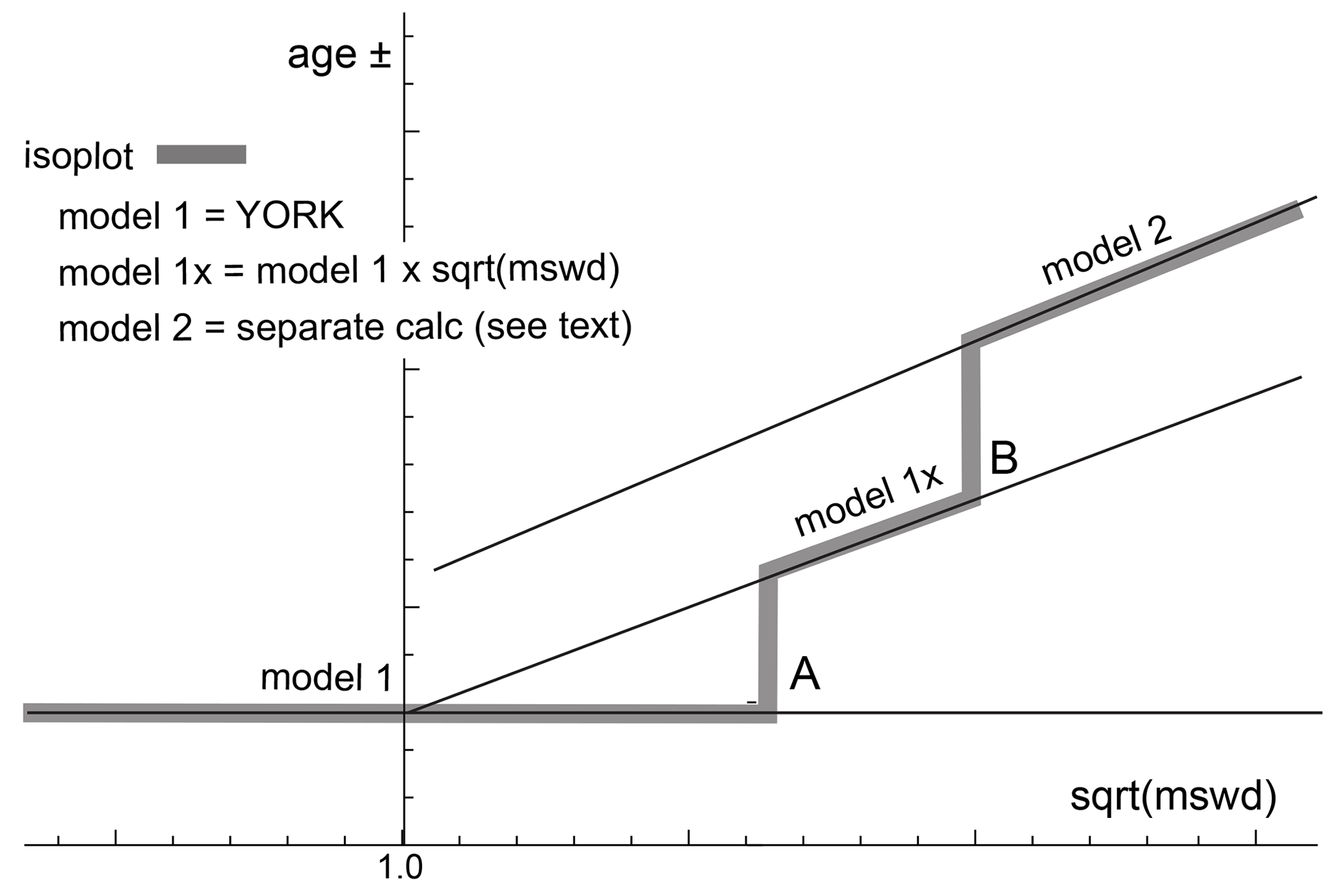
Figure 1 Age uncertainty (age ±) plotted against $\sqrt{\mathtt{\text{mswd}}}$ under the isoplot protocol for a progressively modified dataset (see text and Appendix A). Under the condition of a model 1 fit, the age uncertainty is constant with increasing data scatter (reflected in increasing mswd), until there is a step change in the data treatment at A when the age uncertainty is multiplied by $\sqrt{\mathtt{\text{mswd}}}$. Then, at B, there is another step change in age uncertainty calculation with increasing data scatter forming isoplot model 2 (see text).

What if mswd is greater than the upper limit of the chosen confidence interval? Then the data are considered to have excess scatter, in addition to that accounted for by the data uncertainties (assuming that they are strictly Gaussian)¹. At this point, isoplot, asks the user whether an alternative – model 2 – calculation should be undertaken. This decision point is indicated at A in Fig. 1. If the user declines, isoplot gives results that are referred to here as model 1×, as shown in Fig. 1. The model 1 age uncertainty is multiplied by $\sqrt{\mathtt{\text{mswd}}}$ to reflect the data scatter being more than expected from the data uncertainties alone. With further scatter, the switch is made to model 2, at B in Fig. 1. Alternatively, if the user accepts the switch to model 2, then model 1× is not used, indicated by the vertical line at A extending up to the model 2 line in Fig. 1. The model 2 calculation in isoplot is unrelated to york. The data uncertainties are discarded and the slope of the line through the linear trend is calculated as the geometric mean of the lines calculated by unweighted least squares of y on x and of x on y (see Appendix A).

In summary, then, in isoplot, the calculation of ages and their uncertainties involves a number of decision points based around the concept of mswd that impart significant (and in our view unwelcome) step changes in the way that the data are handled and algorithms applied. To assist in further discussion of these matters, we depart from the language of isoplot at this point, reintroducing the term “errorchron”, counterposed to isochron, following Brooks et al. (1972). The idea is that isochrons have a higher chance of having age significance, while errorchrons have a lower chance. In particular, it seems to be unhelpful for the results of model 2 calculations to be called isochrons as is the case in isoplot, given that there is excess scatter in the data.

1.2 Replacing isoplot

Given that isoplot's implementation of model 1 and 2 line fits is the gold standard of isochron calculations presently, we ask where the problems are and then what can be done to address them. A shortcoming in york stems from the assumption that data uncertainties are strictly Gaussian distributed. In real-world applications, this appears to be too restrictive, with datasets that are likely to have age significance being labelled as errorchrons because mswd is too large. While using york guided by mswd is optimal statistically if data uncertainties are strictly Gaussian, this logic fails once uncertainties are even slightly non-Gaussian (originally Tukey, 1960). In such circumstances, both mswd and least squares methods themselves, like york, become unreliable (e.g. Hampel et al., 1986; Huber, 1981).

Rather than being truly Gaussian, data uncertainties may well be Gaussian distributed in their centres but slightly fat-tailed, distant from the centres. An isotopic dataset looks intuitively acceptable if the data have a central linear “spine” in which scatter is commensurate with stated analytical uncertainty, but this spine is flanked by data of somewhat larger scatter (i.e. excess scatter from the “fat tail”). This excess scatter may originate in the isotopic analysis or as a result of geological disturbance. Age significance in such data manifests primarily via the position of the spine. In the following, we focus on this spine in the data.

Adopting this spine approach, a successful calculation method for a dataset that may not have strictly Gaussian-distributed uncertainties must, firstly, ascertain whether or not such a spine exists in the data – and hence whether calculations yield an isochron or an errorchron. Secondly, in the case of an isochron calculation, the successful method must reliably locate the spine without being perturbed by vagaries in the more scattered data. Classical statistical methods can do neither of these things, tending to be excessively influenced by the data at the extremes of the scatter. However, the field of robust statistics offers calculation methods that can. When a dataset has no excess scatter, reflected in mswd lying within an appropriate χ²-constrained confidence interval, such methods can be devised to retrieve identical (or nearly identical) results to classical statistic methods but, in addition, provide reliable age and age-uncertainty estimates in the presence of excess scatter around a spine. This continuity of operation with increasing mswd contrasts with previous approaches and means that the steps in the isoplot line in Fig. 1, which are certainly undesirable, are circumvented. Moreover, the involvement of potentially unreliable least-squares-based methods, like isoplot model 2, is avoided when the data show excess scatter.

2 An algorithm for isochron calculations

An algorithm is sought that finds a robust straight line through a two-dimensional linear data trend, while converging with the classical statistical approach of york for datasets with consistent scatter (i.e. mswd passes). This section describes the nature of the problem and the theoretical basis for the robust statistical approach that will be adopted. The algorithm adopted

1. determines a preliminary fit of the data, not dependent on vagaries of the data scatter;

2. determines the spine width in relation to this preliminary fit

   • if the spine width is in an acceptable range: isochron, or

   • if the spine width is not in an acceptable range: errorchron;

3. determines a robust fit of the data, starting from the preliminary fit, with this fit converging with york for “good” data.

This algorithm is fleshed out below and then evaluated via simulated datasets and applied to a natural dataset. The central calculation in the algorithm is detailed in Appendix B, and a python implementation is provided in Appendix C.

2.1 Uncertainty distributions and data fitting

Geochronological datasets are collected on the presumption that the isotopic compositions were established via an “event” the age of which is to be estimated. Given the focus here on data with linear trends, even if the effect of the event is recorded perfectly by the samples analysed – the isotopic compositions lying on a line – the actual data are measured with finite precision and so the data inevitably scatter about the trend. An uncertainty probability distribution can be used to describe the form of the data scatter.

Classical statistical methods assume that the underlying uncertainty distribution of a dataset is known, typically taken to be Gaussian. Under the Gaussian assumption, if the analytical uncertainty on the measurements has been appropriately inferred, mswd, the classical statistics parameter used in york to validate an isochron, tests that the scatter of data points is consistent with the inferred uncertainties. But, in general, there is no reason to suppose that a given analytical technique generates a truly Gaussian uncertainty distribution. Even small amounts of geological disturbance destroy the optimality of york. If the uncertainty distribution is not strictly Gaussian, then classical methods of data fitting become sub-optimal or worse.

While there are many possible non-Gaussian uncertainty distributions, this paper is concerned with a situation commonly occurring in datasets, in which the data points form a linear spine with Gaussian-like scatter, but additional scatter is seen in the tails of the distribution. Such a dataset still encodes meaningful age information in its spine, yet it will typically fail an mswd test due to its departure from a Gaussian distribution. In this work, datasets of this nature are modelled using a contaminated Gaussian uncertainty distribution (Gaussian mixture) (e.g. Tukey, 1960). Such distributions are written c %dN, meaning that with a probability (100−c) % the distribution involves a standard deviation, σ, but with a probability c % the distribution has a standard deviation, d σ, both with a mean of zero (see Powell et al., 2002; Maronna et al., 2019, Sect. 2.1). An example is 25 %3N, with c=25 and d=3, so that with 25 % probability the uncertainty is drawn from N(0,3 σ), and 75 % probability drawn from N(0,σ), with the N(0,s) notation indicating a Gaussian distribution with a mean of zero and a standard deviation of s. Such distributions provide excess scatter suitable for developing and evaluating a robust line-fitting calculation. It does not matter if excess scatter in real data is drawn from a different distribution. Note that with the sample sizes provided by most modern geochronological techniques, it is not necessarily possible to test for Gaussian behaviour, or such departures from Gaussian behaviour, although they may be evident on quantile–quantile plots (see below).

2.2 Isochrons and errorchrons

In york, assuming that the data uncertainties are strictly Gaussian distributed, the probability distribution of mswd provides bounds that can be used to distinguish isochrons from errorchrons (e.g. Wendt and Carl, 1991). These bounds come from a 95 % confidence interval on mswd, as discussed in Appendix A. Datasets whose scatter give mswd outside the bounds are deemed to be errorchrons, not isochrons. The focus in this paper is on mswd that is too large, indicating excess scatter. Here, mswd is defined with the residuals, r_k, the distance in y of the data point, k, to the line, e_k, weighted by the uncertainty on this distance, ${\mathit{\sigma }}_{e_k}$:

$$\begin{array}{}\text{(1)}& \mathtt{\text{mswd}}={\displaystyle \frac{\mathrm{1}}{n-\mathrm{2}}}\sum _{k=\mathrm{1}}^n{r}_k^{\mathrm{2}},\end{array}$$

with

$$r_k={\displaystyle \frac{e_k}{{\mathit{\sigma }}_{e_k}}}={\displaystyle \frac{a+b{x}_k-y_k}{b^{\mathrm{2}}{\mathit{\sigma }}_{x_k}^{\mathrm{2}}+{\mathit{\sigma }}_{y_k}^{\mathrm{2}}-\mathrm{2}b{\mathit{\sigma }}_{x_k}{\mathit{\sigma }}_{y_k}{\mathit{\rho }}_{x_k{y}_k}}}.$$

The line being fitted is $y=a+bx$; data point, k, is {x_k,y_k}; the analytical uncertainty on x_k, ${\mathit{\sigma }}_{x_k}$; the analytical uncertainty on y_k, ${\mathit{\sigma }}_{y_k}$; and the correlation between x_k and y_k, ${\mathit{\rho }}_{x_k{y}_k}$ (see derivation of Eq. B4 in Appendix B). Note that the slope, b, appears in the denominator of r_k, as well as the numerator.

If, instead, data uncertainties are c %dN, with unknown c and d, or some other contaminated Gaussian distribution, then there is no equivalent of the mswd argument to say which datasets should give isochrons rather than errorchrons. The approach advocated here is to use a measure that reflects whether the dataset has a linear spine of “good” data within it. The measure suggested, s, coined the spine width, is robust, and is defined as

$$\begin{array}{}\text{(2)}& s=\mathtt{nmad}\left(r\right)=\mathrm{1.4826}\mathtt{median}\left(|r_k-\mathtt{median}(r\left)\right|\right),\end{array}$$

with a normalisation constant², 1.4826. Given that s is based on a median, its magnitude depends on that half of the data that have the smallest absolute values of centred r; in other words, those that would define a spine. If the data were in fact Gaussian distributed, it is expected that s should be in a range about 1 in the same way that mswd is, given that r already involves the analytical uncertainties. The larger the s, greater than 1, the less pronounced the linear spine in the data (or the uncertainties have been underestimated). Whereas the 95 % confidence interval (95 % ci) on mswd for Gaussian-distributed uncertainties comes from a well-established probability distribution, with $(n-\mathrm{2})\mathtt{\text{mswd}}\sim {\mathit{\chi }}_{n-\mathrm{2}}^{\mathrm{2}}$ (e.g Wendt and Carl, 1991), the confidence interval on s needs to be found by simulation (see Appendix D), with the simulated datasets just involving Gaussian-distributed uncertainties. The intervals are given in Table 1.

Table 1 The 95 % confidence intervals for mswd and s, as a function of the number of data points, n (see text).

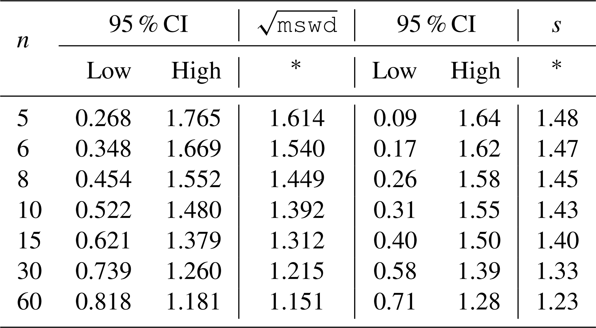
Whereas one-sided confidence intervals are advocated in Appendix A (columns marked with an asterisk in the table), two-sided confidence intervals are also given in the table. Using the column with the asterisk, for example, for a dataset with 10 data points (n=10), the dataset is deemed to yield an isochron if the observed. s is less than 1.43. If s is larger, the dataset gives an errorchron. For isochrons, the age uncertainty is calculated as in Appendix B. For errorchrons, the age uncertainty is not calculated because the data scatter is not consistent with the analytical uncertainties at 95 % confidence, s being larger than the bound.

2.3 A robust statistics approach to isochron calculation

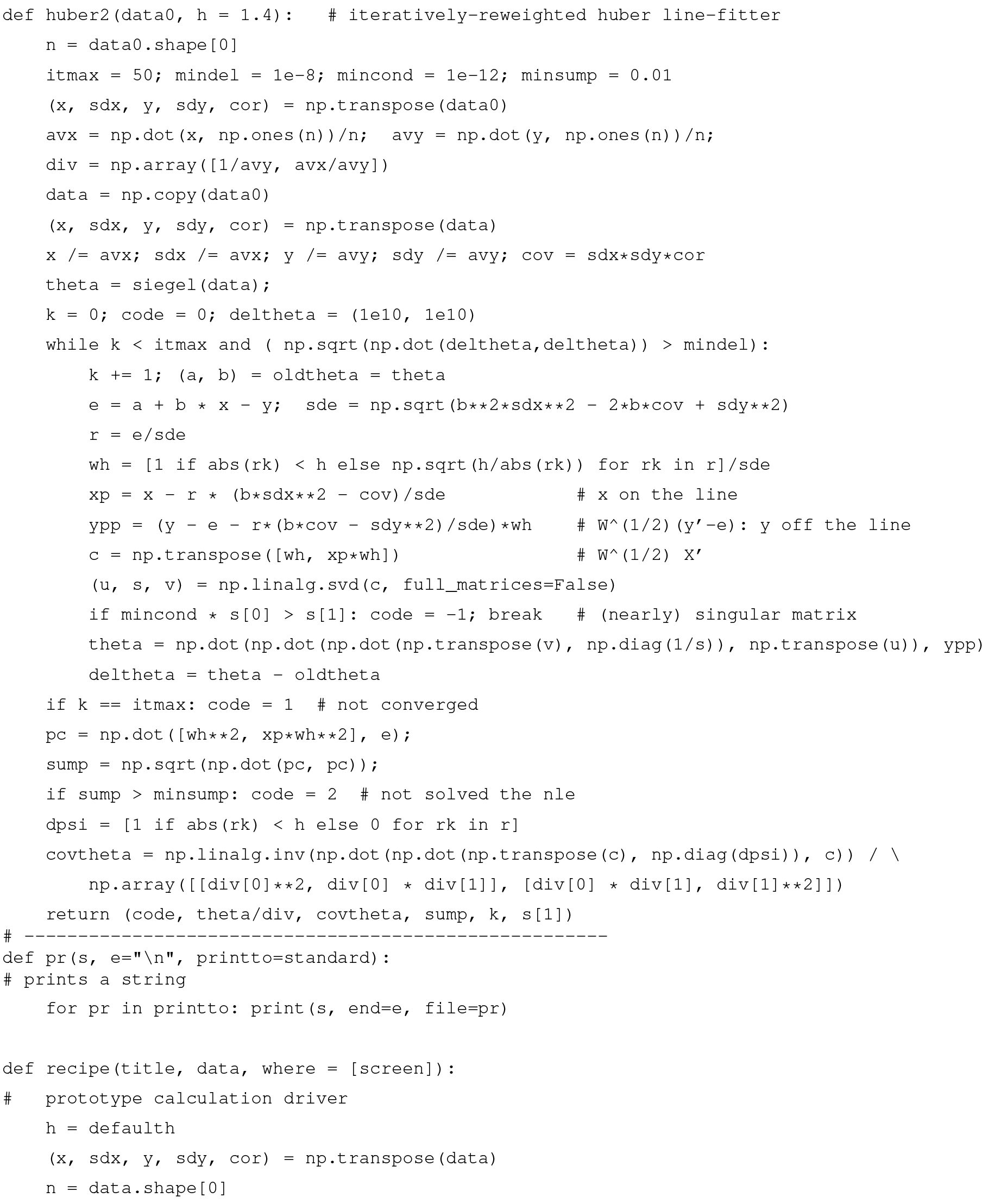
We seek a statistical approach to isochron calculation that is robust (e.g. Huber, 1981; Hampel et al., 1986), meaning that it is not excessively affected by outliers in the data, while having desirable statistical properties, for example, good efficiency (see below). In addition, we require the approach to converge to york for a “good” dataset, one with a near-Gaussian uncertainty distribution, allowing seamless compatibility with classical data interpretation. The overall approach adopted will be referred to as spine, involving the use of spine width for isochron–errorchron distinction, combined with robust line fitting. The line fitting is based on the approach of Huber (1981), as outlined in Maronna et al. (2019, Sect. 2.2.2). Whereas most robust line-fitting methods use the scatter of the data as a scale, data uncertainties having been discarded (e.g. Powell et al., 2002); here, the data uncertainties are used. This is necessary in order to preserve continuity of the results with york, in which the data uncertainties are an integral part of the calculation.

In both the Huber approach in spine and in york, a straight line is fitted to a dataset by minimising a function of the residuals, r_k. In the case of york, this is just the mswd (Eq. 1). Since isochron data are generally bivariate with correlated analytical uncertainties in x and y, the analytical uncertainty in data point k can be represented as an ellipse as in Fig. 2. The absolute value of the residual for data point, k, r_k, is in fact the scaling factor for the size of the ellipse required to expand it or reduce it until it touches the best-fit line (Fig. 2).

The function that is minimised to find the best-fit line can be written ∑ρ(r_k) for both york and spine. Whereas in york, $\mathit{\rho }\left(r_k\right)=r_k^{\mathrm{2}}$ for all r_k, in spine $\mathit{\rho }\left(r_k\right)=r_k^{\mathrm{2}}$ near the centre of the uncertainty distribution (as in york) but downweights data points for which the absolute value of the residual is greater than a cut-off value, h. Thus, in spine, and in Fig. 3, the Huber ρ is

$$\begin{array}{}\text{(3)}& \mathit{\rho }\left(r_k\right)=\left\{\begin{array}{lrl}\mathrm{2}h{r}_k-h^{\mathrm{2}}& & r_k<-h\\ r_k^{\mathrm{2}}& \mathrm{if}& -h<r_k<h\\ \mathrm{2}h{r}_k-h^{\mathrm{2}}& & r_k>h.\end{array}\right.\end{array}$$

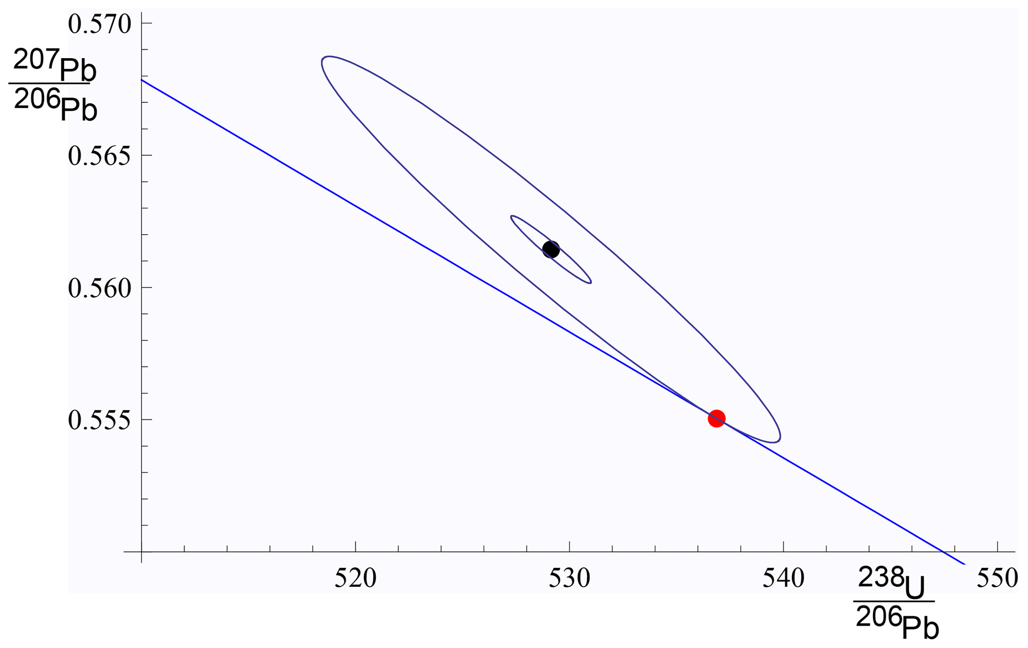
Figure 2 For an example data point, {x_k,y_k}, the inner ellipse is calculated with the analytical uncertainties, V_k, at the 1σ level (in black). Given a line, $y=a+bx$ (in blue), the ellipse must be drawn at the $\left|r_k\right|\mathit{\sigma }$ level (in red) to touch the line, in this case $\left|r_k\right|=\mathrm{5.73}$. The data point is x_k=529.14, y_k=0.5614, and ${\mathit{\sigma }}_{x_k}=\mathrm{1.870}$, ${\mathit{\sigma }}_{y_k}=\mathrm{0.00127}$, and ${\mathit{\rho }}_{x_k{y}_k}=-\mathrm{0.967}$. The line is $y=\mathrm{0.8108}-\mathrm{0.0004764}x$.

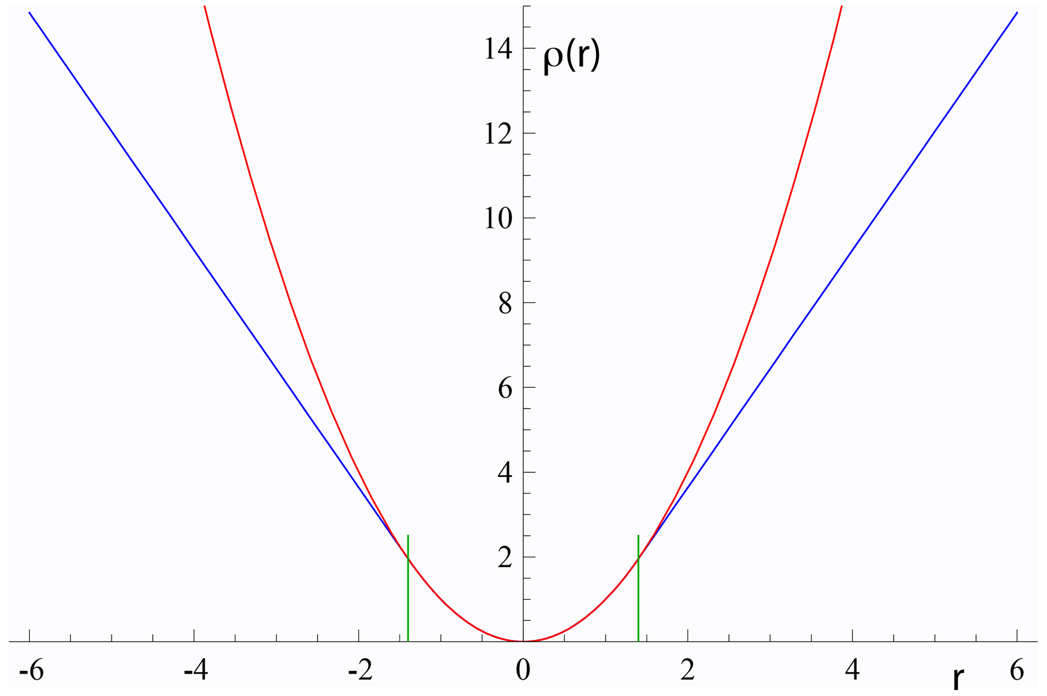
Figure 3 Plots of ρ(r) against r for york in red (r²) and for Huber in spine (Eq. 3) in blue. The two curves are coincident for $\left|r\right|<h$, with h=1.4 the vertical green lines. See text.

In spine, for residuals that have an absolute value less than an adjustable constant, h, the contribution to the sum being minimised is the same as for york, but it is linear in the residual for larger absolute values. Note that as h becomes larger and larger, spine converges to york. The value to use for h is discussed in Maronna et al. (2019)³.

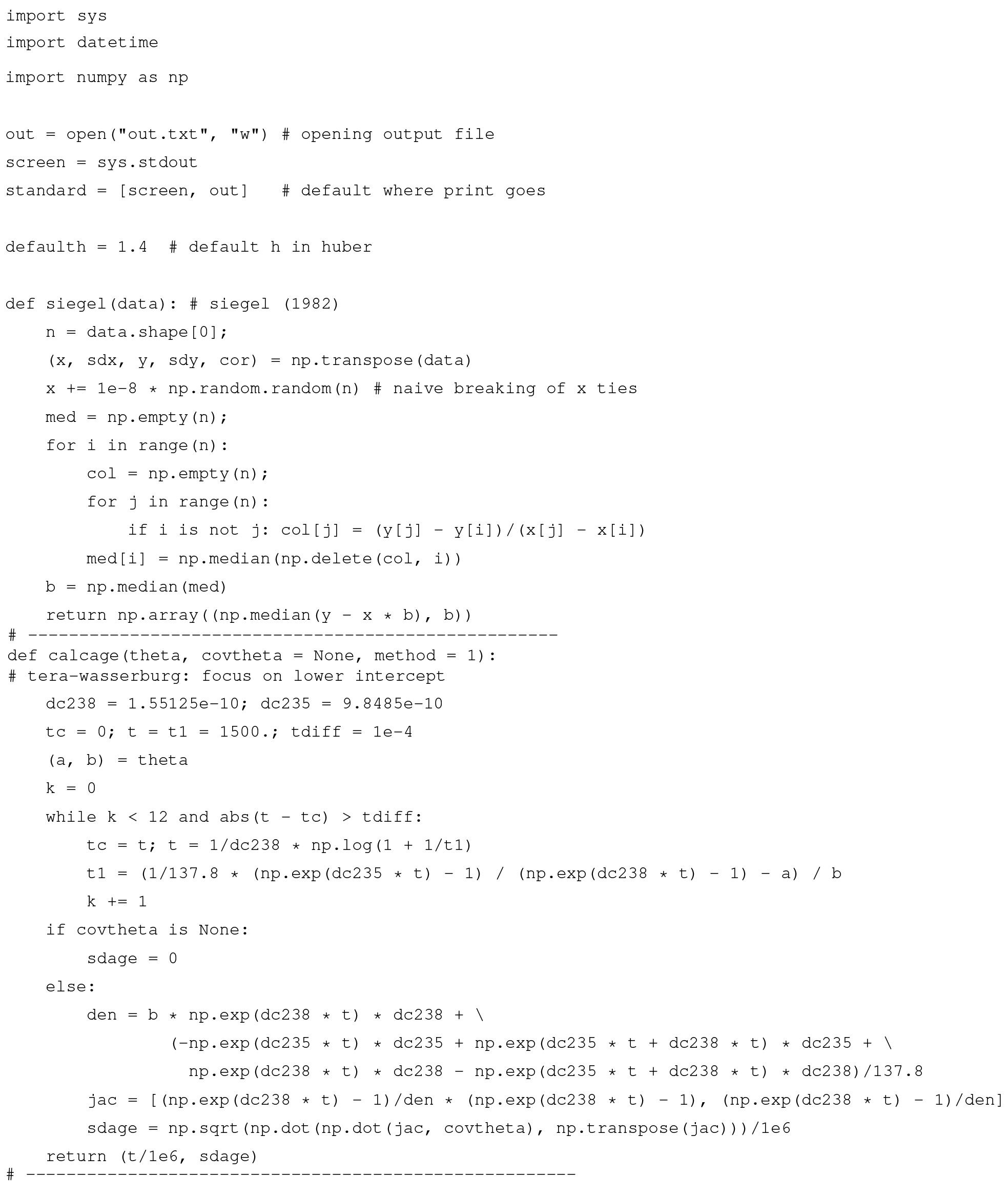
The iteration developed in Appendix B minimises ∑_kρ(r_k) with respect to the unknown, θ, a two-element column vector, {a,b}^T in the line equation, $y=a+bx$. The iteration is applicable to spine and also york. As a starting point of the iteration, data are fit for θ with siegel (Siegel, 1982), which is highly robust toward excess scatter. However, siegel is much less efficient than spine (see below), so spine is a better ultimate estimator. A full iteration is envisaged in Appendix B. Once θ is calculated, the measure of scatter used to distinguish an isochron from an errorchron can be calculated using Table 1. If an isochron is deemed to have been calculated, the uncertainty on θ, V_θ, can be found, as outlined in Appendix B.

The spine algorithm can be summarised as follows:

1. determine a preliminary fit of the data using siegel;

2. determine the spine width using nmad

   • if the spine width is in an acceptable range, from col. 6 in Table 1: isochron, or

   • if the spine width is not in the acceptable range: errorchron;

3. determine a robust fit of the data, minimising ∑ρ(r_k), with the Huber ρ(r_k) (Eq. 3) starting from the siegel estimate of θ.

2.4 Application of spine to simulated datasets

Assessing algorithms for data fitting is best done using simulated datasets, so that the true “age” represented by the data is known. In this case, datasets were generated by drawing data points from a range of uncertainty distributions, all centred on a linear trend reflecting an age of 4 Ma. Full details are provided in Appendix D. Two features of the datasets are varied: the number of data points in the dataset and the uncertainty structure adopted, the latter via varying c and d in c %dN. The algorithm is assessed in terms of its ability to retrieve the specified age of the linear trend on which the simulated datasets are built and on the uncertainty in the age.

Given that the datasets investigated have fat-tailed contaminated Gaussian uncertainty distributions, the focus is on the effect of excess scatter in the data or, in other words, data scatter over and above what is expected for Gaussian data uncertainties. Nevertheless, a small proportion of datasets do have small scatter, giving s which is below the lower bound for that number of data points.

The analysis below compares the results of york, applied only to those simulated datasets that lie within the mswd bounds, with the results of spine applied to those datasets that lie within the spine width (s) bounds. The greatest majority of the former are included in the latter, e.g. > 97 % for n=10). Importantly, however, spine typically identifies reliable age information in many more datasets than york. In Table 2, m % excl and s % excl are the percentage of simulated datasets excluded on the basis of the mswd and s bounds, respectively.

Table 2 Percentage of simulated datasets excluded by the mswd and s bounds given in Table 1 (see text).

Note that, for example, for n=10, datasets drawn from 5 %3N, in fact have 100(10^0.95)=59.9 % of the datasets having all uncertainties Gaussian, while 40.1 % have at least one uncertainty drawn from 3 times the Gaussian (3N). For 25 %3N, 5.6 % are Gaussian only, and for 10 %10N, it is 34.9 %. The leftmost columns are 2.5 % by definition.

A 95 % confidence interval on age can be found by ordering the list of ages calculated for the datasets, selecting the lower limit at the 2.5 % point in the list, and the upper limit at the 97.5 % point. For datasets that lie within the s bound in spine or mswd bound in york, the 95 % confidence intervals on ages are essentially the same, even though a much larger proportion of datasets lie within bounds using spine than using york. A comparison of ages can also be made between york and spine for simulated datasets that lie outside the mswd bounds. For n=10 and Gaussian-distributed data, the 95 % confidence interval is ±0.021 Ma for both york and spine, but for 5 %3N, 25 %3N, and 10 %10N, the 95 % confidence interval on the york ages are ± 0.035, ±0.040, and ±0.092 Ma, respectively, while the spine ages are ±0.027, ±0.034, and ±0.034 Ma. The differences between the ages given by the two methods, normalised by the uncertainties on the spine ages, are ±1.62, ±1.63, and ±5.54. Comparison of the intervals shows that the mswd bounds are relevant to the application of york, in that generally it does not work well outside the bounds, while indicating that spine is (much) more reliable for age determination for such datasets.

Considering age uncertainty, it might be expected that the uncertainties suffer from the excess scatter in the data in datasets that yield an errorchron with york but an isochron with spine.This appears not to be the case, but there is a small degradation in the age uncertainties retrieved caused by an unavoidable efficiency loss using spine. Efficiency at the Gaussian distribution is the ratio of the variance obtained by the optimal estimator (york) divided by the variance using the chosen robust estimator (in this case, spine). spine involves an efficiency loss at the Gaussian distribution, which is illustrated in Fig. 4 via kernel density estimate (kde) plots of the age uncertainties calculated for simulated datasets with n=10 and Gaussian-distributed uncertainties. The kde plots are probability distributions akin to smoothed histograms (Wand and Jones, 1995). The red curve is the kde for datasets that have all $\left|r_k\right|<h$, as would be given by york on datasets with Gaussian-distributed uncertainties. The blue curve is the kde for all datasets with at least one $\left|r_k\right|>h$. The overall kde, in black, is the kde of all of the datasets in the red and blue kde, in observed proportion, about 30 % to 70 %. The efficiency loss of spine is reflected in the displacement of the black curve to slightly higher age uncertainty than the red curve. The relationships shown in Fig. 4 for n=10 can be seen for other n in Fig. 5. The pairs of red and black lines correspond to and have the same meaning as the red and black lines in Fig. 4. As expected, the distribution of age uncertainties moves towards larger values as the sample size n decreases.

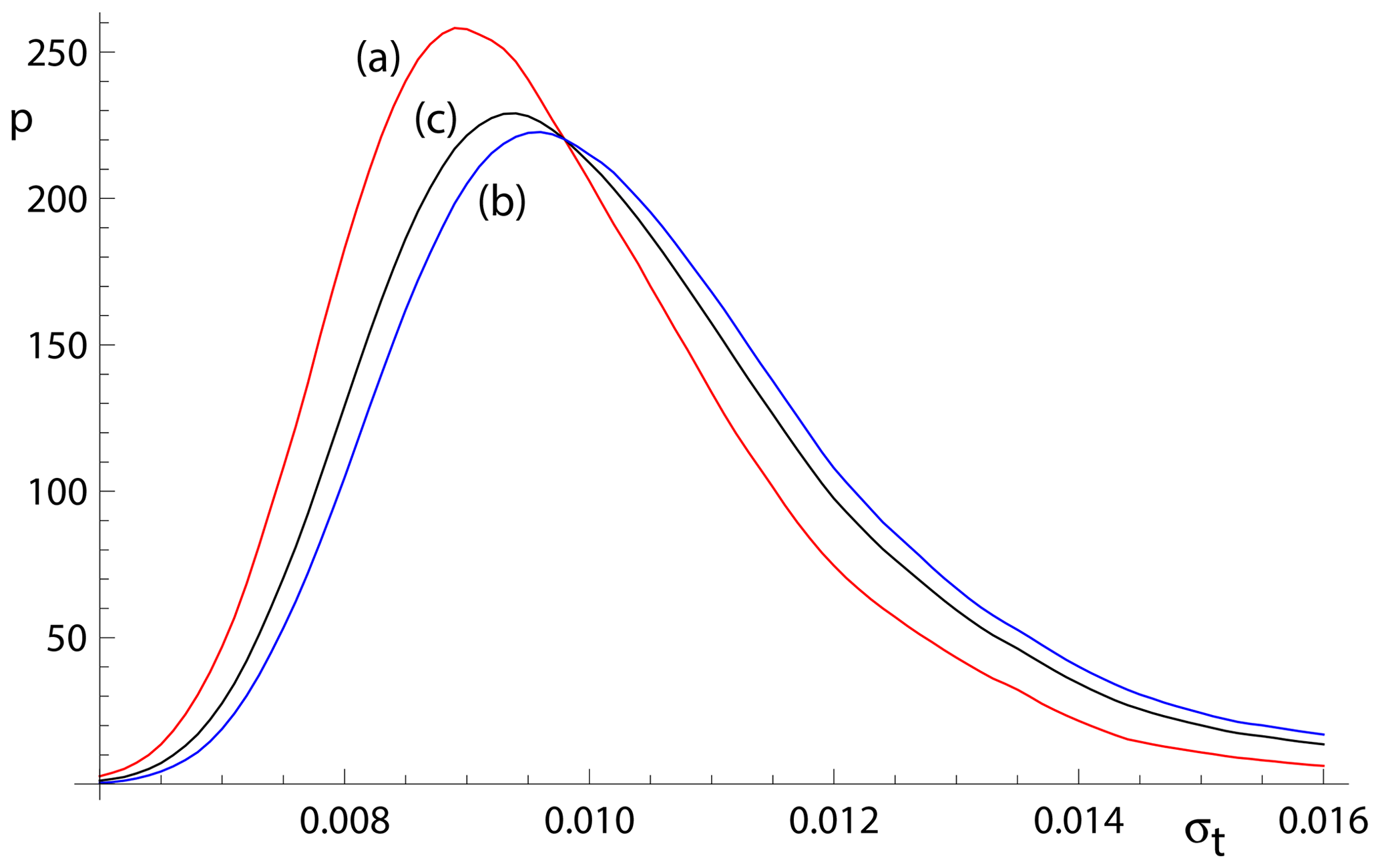
Figure 4 Kernel density estimates (kde) for age uncertainty calculated with spine on 10 000 simulated datasets with n=10 and Gaussian-distributed uncertainties. (a) Those datasets for which all $\left|r_k\right|<h$ (in red); (b) those datasets for which at least one $\left|r_k\right|>h$ (in blue), and (c) overall result combining panels (a) and (b) in observed proportion (in black).

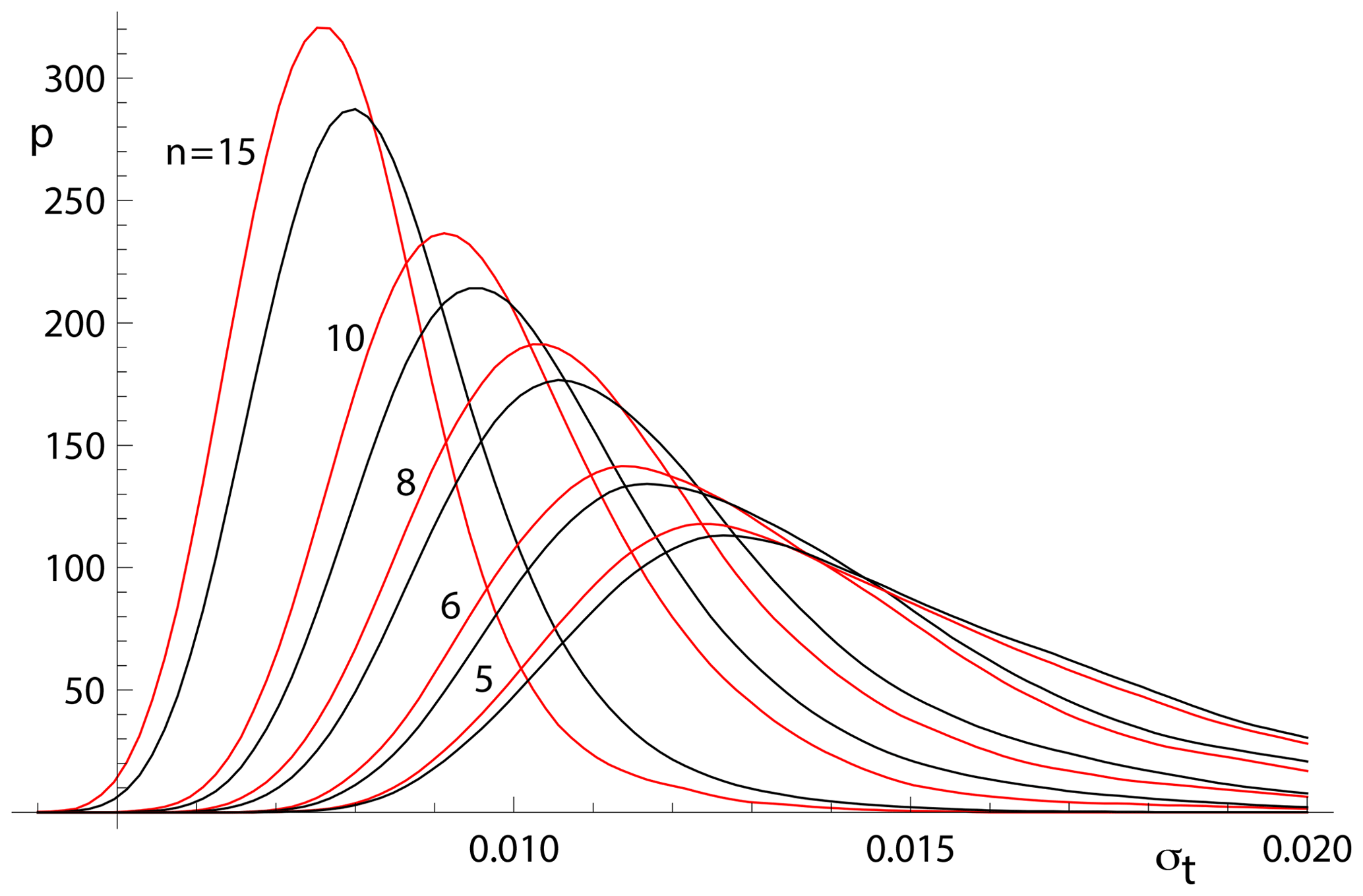
Figure 5 Kernel density estimates for age uncertainty calculated with spine on 10 000 simulated datasets with a range of n values and Gaussian-distributed uncertainties. In each case, the kde for those datasets for which all $\left|r_k\right|<h$ is in red and the overall kde is in black.

Whereas spine involves an efficiency loss at the Gaussian distribution, it performs better – i.e. it is much more robust – than york for data from contaminated Gaussian distributions (e.g. Maronna et al., 2019, Table 2.2). The ability of spine to retrieve age uncertainty information for such data varies with the probability and scale of the contamination, as shown in Fig. 6. Not unexpectedly, the more seriously contaminated distributions (25 %3N and 10 %10N) involve a greater displacement of the kde to higher age uncertainty than the more weakly contaminated 5 %3N distribution. Although the displacement of the blue curves from the black curve is real, the ability of spine to retrieve age uncertainties from datasets with contaminated distributions is good.

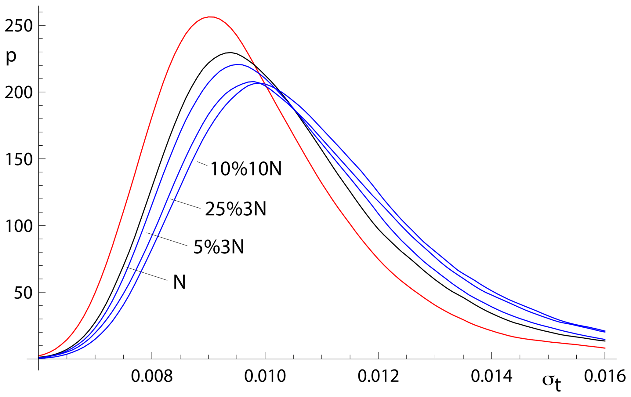
Figure 6 Kernel density estimates for age uncertainty calculated with spine on 10 000 simulated datasets with n=10 and several uncertainty structures. The kde for those datasets for which all $\left|r_k\right|<h$ is in red, the kde for datasets with Gaussian-distributed uncertainties is in black, and the kde for all of the datasets for 5 %3N, 25 %3N, and 10 %10N, respectively, are in blue.

2.5 Application of spine to a natural dataset

In order to show the real-world utility of spine, we consider data for a carbonate flowstone from the Riversleigh World Heritage fossil site in Queensland, Australia (Sample 0708). Isotope dilution U–Pb data for the bulk sample were previously published by Woodhead et al. (2016) providing a model 2 isochron with an age of 13.72±0.12 Ma and mswd of 3.7. The new data presented here were obtained by laser ablation icpms on the same sample using methods outlined and published in Woodhead and Petrus (2019). Such datasets are typically larger with little error correlation (rounder error ellipses) but with larger uncertainties than isotope dilution data. These new data define an errorchron under the york assumptions, with mswd = 1.68, and a model 2 age of 13.68±0.31 Ma. These data might therefore be rejected under the mswd criterion despite exhibiting a well-developed linear trend. With spine, s=1.24, within the s range for an isochron, the age is 13.69±0.26 Ma (± is 1.96σ). The data for 0708 are plotted in Fig. 7, with 95 % confidence ellipses on the data points. Further calculations with this sample, comparing the results of our new algorithm with existing approaches are presented in Appendix A.

Figure 7 Laser ablation example 0708. See text.

With 0708, the spine and isoplot ages are very similar, but mswd suggests an errorchron, so there is excess scatter on this basis. Quantile–quantile plots can be used to show the nature of the distribution of the residuals that contribute to such excess scatter. Here, Fig. 8, the ordered residuals normalised to 𝚗𝚖𝚊𝚍(r) are plotted against the quantiles of the standard Gaussian distribution, N(0,1) (see Fox, 2016, Sect. 3.1.3). The normalisation means that if the residuals are Gaussian distributed, they should plot close to a line of unit slope through the origin. The figure also includes 95 % pointwise confidence intervals (dashed blue lines). The figure suggests that the residuals are in fact effectively Gaussian distributed, lying between the dashed blue lines (and mswd has been too sensitive in flagging that the residuals are not Gaussian distributed).

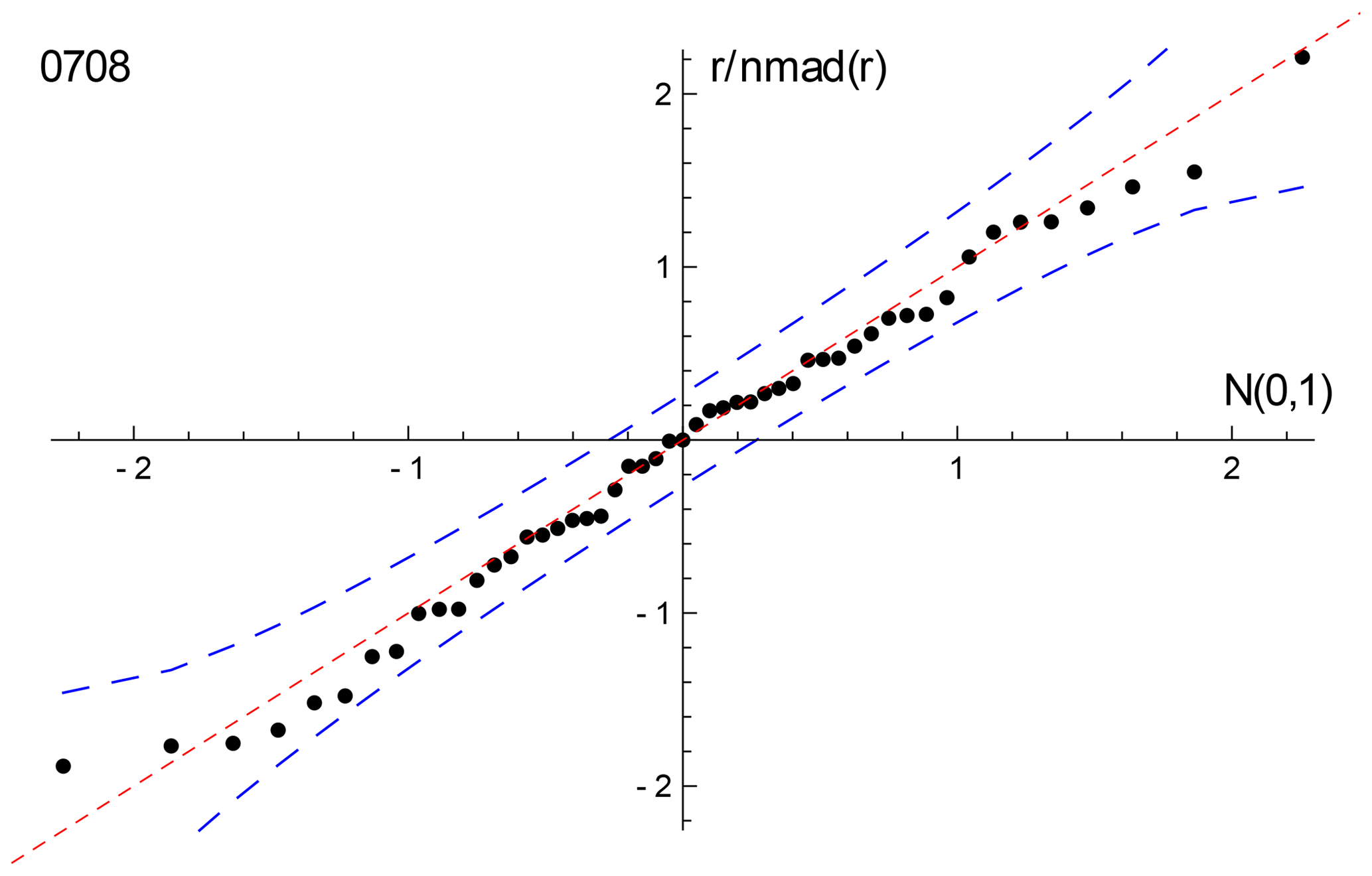
Figure 8 Quantile–quantile plot for sample 0708, using the siegel fit of the data to calculate the residuals to plot. The dashed red line has unit slope through the origin; the dashed blue lines are the 95 % pointwise confidence intervals. See text.

Generally, geochronological datasets do not have obvious outliers – they might be “cleaned” of isolated data points before an age calculation, or the dataset might even be discarded. But many of the simulated datasets from contaminated Gaussian distributions, as used above, do contain outliers. In Appendix E, an example of a simulated dataset with outliers (from 25 %3N) is used to show how york and spine behave and what a quantile–quantile plot looks like in those circumstances.

3 Discussion and conclusions

This work was motivated by the belief that many isotopic datasets contain meaningful age information that cannot be identified using classical statistical methods and may therefore be discarded or discounted. In such cases, the age information is contained in a linear spine in the data, but the data also contain scatter that is inconsistent with a Gaussian uncertainty distribution, having fatter tails than Gaussian. A statistical test based on the spine width is devised, akin to using mswd in classical methods, allowing an isochron–errorchron distinction to be made. Many datasets that give isochrons based on the spine width, give errorchrons under the assumption of a strict Gaussian uncertainty distribution. A statistically robust isochron calculation method is able to retrieve this age information and to provide appropriate uncertainty estimates. Calculated ages and age uncertainties are more reliable than isoplot ones for data with excess scatter. Contaminated Gaussian distributions provide a model for a type of dataset with excess scatter relative to a strictly Gaussian-distributed one. The robust isochron method presented in this work can however be applied in general to data which are Gaussian distributed only in the central spine of the uncertainty distribution, with non-Gaussian scatter occurring in the tails, arising from analytical or geological uncertainty. Indeed, it can be applied to any dataset with a well-developed spine in the data.

In most robust statistics data-fitting approaches, the formal uncertainties output during data measurement are ignored. Instead, the scale used in the data fitting is derived from the scatter in the data, an approach adopted by Powell et al. (2002). The new approach followed here does include the data measurement uncertainties, and this allows the results to converge on those of york when the data lack excess scatter. This provides compatibility with older “good” datasets processed using the classical statistical approach but, going forward, allows age information to be extracted from a much wider range of datasets which might otherwise be rejected for having mswd greater than the isochron cutoff.

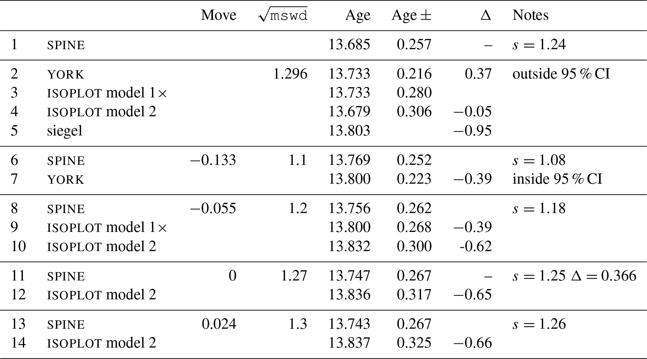
A problem with spine, shared with york, is that the effect of high-leverage data is not taken into account. Such data are easily recognised in x–y plots, when a small proportion of the data – even one data point – is separated from the main body of the data along the trend through the data. Data fitting tends to be overly constrained to fit high-leverage data, giving them small residuals, even if the best fit of the main body of the data alone would give the high-leverage data larger residuals. In 0708, the point at highest x is of relatively high leverage (hat = 0.171). Robust approaches have been developed to handle high-leverage data, e.g. Maronna et al. (2019, chap. 5), but are not yet developed for the situation where the data uncertainties are taken into account, nor for the relatively small datasets that are typical of geochronological studies (cf. Fig. 7). Huber and Rochetti (2009, chap. 7), have a counter view advocating data assessment, rather than aiming for a black-box method to try and automatically safeguard against the potentially deleterious effect of high-leverage data, an approach we suggest here. In the case of the relatively high-leverage data point in 0708, omitting this data point gives 13.75±0.27 Ma (compare row 11 with row 1 in the table in Appendix A), within uncertainty of the age including this data point.

Appendix A: Algorithms and applications to sample 0708

Here, some results of calculations for sample 0708 are collected, used in Fig. 7, along with some related algorithmic details.

A1 Thought experiment in Fig. 1

The thought experiment sketched in Fig. 1 aimed to show the consequence for isoplot behaviour of the modification of the observed data in a dataset to reduce or increase the scatter about the linear trend. The calculated equivalent of Fig. 1 for sample 0708 is shown in Fig. A1, including also the corresponding spine results. In calculating the figure, the modification of the dataset is achieved by first taking the data points with their attendant error ellipses (i.e. covariance matrices) and moving them all in to lie on the linear trend, considered as fixed by a york calculation. Then the points and ellipses are considered to be displaced away from the trend. This is “move” in the table below, going from −1, when the points lie on the trend, through 0, with the points as in the original data, to positive when displaced further away from the trend. “Move” varies more or less linearly with $\sqrt{\mathtt{\text{mswd}}}$ from −0.133 at the left edge of the figure to 0.064 on the right edge; the spine width changes from 1.08 to 1.32 across the figure. For these calculations, the last line in the dataset is omitted as it is of relatively high leverage (hat = 0.171), not wishing this data point to affect the results.

Figure A1 Age uncertainty (age ±) plotted against $\sqrt{\mathtt{\text{mswd}}}$ under the isoplot protocol for the progressively modified dataset, 0708 (see text). In model 1, the age uncertainty is constant with increasing data scatter (reflected in increasing mswd), until there is a step change in age uncertainty at A when the ± is multiplied by $\sqrt{\mathtt{\text{mswd}}}$. Then, at B, there is another step change with further increase of data scatter to model 2 (see text). The location of the step at A is based on a 95 % confidence interval for mswd (discussed below), whereas the $\sqrt{\mathtt{\text{mswd}}}$ position of the step at B is arbitrary. The y axis is drawn at the $\sqrt{\mathtt{\text{mswd}}}$ of the actual data, 1.27 (i.e. no modification of the data). See text.

In the figure, extending from the left, through mswd = 1, to A, the isoplot age uncertainty (model 1, i.e. york) is constant because the data scatter is consistent with the data uncertainties. Through this range, the spine age uncertainty is above the model 1 line because of the efficiency loss embodied in spine, as shown in Figs. 4–5. However, after the age uncertainty steps with increasing mswd, to the right of the diagram, the spine age uncertainty is smaller than the model 1× and model 2 age uncertainty. This is because spine gives an isochron on the basis of spine width up to C at $\sqrt{\mathtt{\text{mswd}}}\approx \mathrm{1.3}$, whereas model 2 is an errorchron on the basis of the assumption of strictly Gaussian data uncertainties. The small steps in the spine age uncertainty line are an artefact of the approximation used in the calculation of the age uncertainty; see Appendix B.

In the top part of Table A1, the results for spine and for isoplot are summarised. The Δ column gives the change to the age from the spine age, normalised by the uncertainty on the spine age. Below the double line in the table are some results from the above thought experiment, Fig. A1.

Table A1 Summary of results used in constructing Fig. A1 (see text).

Additional algorithmic details for isoplot follow next, in part related to the above thought experiment.

A2 isoplot model 1

In the isoplot model 1 calculation, i.e. in york, a decision has to be made about the confidence interval on mswd that is used to denote the range of data scatter (i.e. mswd) that is considered to be accounted for by the data uncertainties, without need to either multiply the age uncertainty by $\sqrt{\mathtt{\text{mswd}}}$ (i.e. model 1×) or switch directly to an alternative calculation (which is model 2 in isoplot). On the understanding that data uncertainties are correctly assigned, a one-sided confidence interval on mswd can be adopted, acknowledging that mswd is not being used to identify the case where assigned data uncertainties are too large or too small. The upper end of the confidence interval on mswd is where excess scatter is considered to start, a conventional choice being derived from a 95 % confidence interval. Note that there is no argument that this should be at 𝚖𝚜𝚠𝚍=1 (cf. Dickin, 2005, p37), unless the number of data points is huge. Even for a dataset of 50 data points, the 95 % confidence interval on mswd extends to 1.36. In terms of the probability of fit measure used in isoplot, this is $\mathrm{100}-\mathrm{95}=\mathrm{5}$ %. It might be noted that the naming of probability of fit seems unhelpful – it is clearer to focus on mswd.

A3 isoplot model 2

The so-called error-in-variables (eiv) or measurement-error problem is avoided in york because the uncertainty in the x variable is taken into account explicitly. If it was not, then eiv results in the calculated slope being biased downwards and the approach being inconsistent (e.g. Fuller, 1987).

In the isoplot model 2 calculation, eiv is avoided, even though the data uncertainties are discarded, by making the slope of the line through the data be the geometric mean of the slopes of ordinary least squares of y on x, b_yx, and x on y, 1∕b_xy. These are

$$b_{yx}={\displaystyle \frac{\sum (x_k-\stackrel{\mathrm{‾}}{x})(y_k-\stackrel{\mathrm{‾}}{y})}{\sum (x_k-\stackrel{\mathrm{‾}}{x}{)}^{\mathrm{2}}}}$$

and

$${\displaystyle \frac{\mathrm{1}}{b_{xy}}}={\displaystyle \frac{\sum (x_k-\stackrel{\mathrm{‾}}{x})(y_k-\stackrel{\mathrm{‾}}{y})}{\sum (y_k-\stackrel{\mathrm{‾}}{y}{)}^{\mathrm{2}}}},$$

with $\stackrel{\mathrm{‾}}{x}=\frac{\mathrm{1}}{n}\sum x_k$ and $\stackrel{\mathrm{‾}}{y}=\frac{\mathrm{1}}{n}\sum y_k$. Then

$$b=\pm \sqrt{b_{yx}{b}_{xy}}=\pm \sqrt{{\displaystyle \frac{\sum (y_k-\stackrel{\mathrm{‾}}{y}{)}^{\mathrm{2}}}{\sum (x_k-\stackrel{\mathrm{‾}}{x}{)}^{\mathrm{2}}}}}$$

and

$$a=\stackrel{\mathrm{‾}}{y}-b\stackrel{\mathrm{‾}}{x},$$

with, in this case, the sign of the square root being negative. The calculation in isoplot does not use this explicit formula, instead adopting an algebraic equivalent that allows the york iteration to be used.

A4 isoplot robust

In isoplot, there is an option to use a robust isochron calculation method. The two available have high breakdown point but low efficiency (e.g. Huber, 1981, Sect. 1.2.3). The second method (Siegel, 1982) can be considered to supersede the first. In fact, here, siegel is used in the implementation of spine as a starting point for the iteration (see Appendix C). The fit of the data for sample 0708 with siegel is given in line 5 of the table.

Appendix B: Iteration in spine

The spine algorithm involves minimising ∑_kρ(r_k) with respect to the unknown, θ, a two-element column vector, {a,b}^T in the line equation, $y=a+bx$, in order to fit the data. The residual, r_k on data point k is defined below, and the function ρ is defined in Eq. (3) in the main text. The spine algorithm subsumes york.

Writing the kth data point as {x_k,y_k}, generally the isotopic data used in isochron calculations involve uncertainties in both x_k and y_k, and commonly the x_k and y_k are also correlated. These can be represented by a covariance matrix, V_k,

$$\begin{array}{}\text{(B1)}& V_k=\left[\begin{array}{cc}{\mathit{\sigma }}_{x_k}^{\mathrm{2}}& {\mathit{\sigma }}_{x_k}{\mathit{\sigma }}_{y_k}{\mathit{\rho }}_{x_k{y}_k}\\ {\mathit{\sigma }}_{x_k}{\mathit{\sigma }}_{y_k}{\mathit{\rho }}_{x_k{y}_k}& {\mathit{\sigma }}_{y_k}^{\mathrm{2}},\end{array}\right]\end{array}$$

in which ${\mathit{\sigma }}_{x_k}$ is the standard deviation on x_k, ${\mathit{\sigma }}_{y_k}$ the standard deviation on y_k, ${\mathit{\sigma }}_{x_k}{\mathit{\sigma }}_{y_k}{\mathit{\rho }}_{x_k{y}_k}$ the covariance between x_k and y_k, and ${\mathit{\rho }}_{x_k{y}_k}$ the correlation coefficient between x_k and y_k. The covariance matrix can be represented by an ellipse around the data point in an x–y diagram, as illustrated in Fig. 2. The residual, r_k, a measure of the distance of the point {x_k,y_k} to the line, is calculated from the coordinates of the data points, {x_k,y_k}, and their uncertainties in V_k, by

$$\begin{array}{}\text{(B2)}& r_k={\displaystyle \frac{e_k}{{\mathit{\sigma }}_{e_k}}},\end{array}$$

in which e_k is the distance of the data point from the line, $e_k=a+b{x}_k-y_k$, and ${\mathit{\sigma }}_{e_k}$ is the standard deviation on e_k. The standard deviation, ${\mathit{\sigma }}_{e_k}$, is calculated by error propagation using V_k:

$$\begin{array}{}\text{(B3)}& \begin{array}{rl}{\mathit{\sigma }}_{e_k}^{\mathrm{2}}& =\left\{{\displaystyle \frac{\partial e_k}{\partial x_k}},{\displaystyle \frac{\partial e_k}{\partial y_k}}\right\}{V}_k{\left\{{\displaystyle \frac{\partial e_k}{\partial x_k}},{\displaystyle \frac{\partial e_k}{\partial y_k}}\right\}}^{\mathrm{T}}\\ & =b^{\mathrm{2}}{\mathit{\sigma }}_{x_k}^{\mathrm{2}}+{\mathit{\sigma }}_{y_k}^{\mathrm{2}}-\mathrm{2}b{\mathit{\sigma }}_{x_k}{\mathit{\sigma }}_{y_k}{\mathit{\rho }}_{x_k{y}_k},\end{array}\end{array}$$

with the term in curly brackets evaluating to $\left\{b,-\mathrm{1}\right\}$. The residual is then

$$\begin{array}{}\text{(B4)}& r_k={\displaystyle \frac{e_k}{{\mathit{\sigma }}_{e_k}}}={\displaystyle \frac{a+b{x}_k-y_k}{\sqrt{b^{\mathrm{2}}{\mathit{\sigma }}_{x_k}^{\mathrm{2}}+{\mathit{\sigma }}_{y_k}^{\mathrm{2}}-\mathrm{2}b{\mathit{\sigma }}_{x_k}{\mathit{\sigma }}_{y_k}{\mathit{\rho }}_{x_k{y}_k}}}}.\end{array}$$

In matrix form, the residuals can be written as a column vector, r

$$\begin{array}{}\text{(B5)}& \mathit{r}={\mathbf{W}}_e\mathbf{e}={\mathbf{W}}_e(\mathbf{X}\mathit{\theta }-\mathbf{y}),\end{array}$$

with W_e a diagonal matrix with kkth element, $\mathrm{1}/{\mathit{\sigma }}_{e_k}$.

The minimisation of ∑_kρ(r_k) is iterative, starting from a robust but low efficiency estimate of the line, for example, using Siegel (1982). The minimisation is undertaken using the fact that, at the minimum, the derivative of ∑ρ(r_k) with respect to θ is zero. Defining

$$\begin{array}{}\text{(B6)}& \mathrm{2}\mathit{\psi }\left(r_k\right)={\displaystyle \frac{\partial \mathit{\rho }\left(r_k\right)}{\partial r_k}},\end{array}$$

this function, for the Huber (1981) approach, from Eq. (3), is

$$\begin{array}{}\text{(B7)}& \mathit{\psi }\left(r_k\right)=\left\{\begin{array}{rrl}-h& & r_k<-h\\ r_k& \mathrm{if}& -h<r_k<h\\ h& & r_k>h.\end{array}\right.\end{array}$$

For york, ψ(r_k)=r_k, equivalent to spine with large h.

At the minimum of ∑ρ(r_k),

$$\begin{array}{}\text{(B8)}& \begin{array}{rl}\sum _k{\displaystyle \frac{\partial \mathit{\rho }\left(r_k\right)}{\partial \mathit{\theta }}}=\mathrm{0}& =\sum _k\left({\displaystyle \frac{\partial \mathit{\rho }\left(r_k\right)}{\partial r_k}}\right)\left({\displaystyle \frac{\partial r_k}{\partial \mathit{\theta }}}\right)=\sum _k\mathit{\psi }\left(r_k\right)\left({\displaystyle \frac{\partial r_k}{\partial \mathit{\theta }}}\right)\\ & =\sum _k\mathit{\psi }\left(r_k\right){\displaystyle \frac{\mathrm{1}}{{\mathit{\sigma }}_{e_k}}}\left\{\left({\displaystyle \frac{\partial e_k}{\partial \mathit{\theta }}}\right)-r_k\left({\displaystyle \frac{\partial {\mathit{\sigma }}_{e_k}}{\partial \mathit{\theta }}}\right)\right\}\end{array}.\end{array}$$

In the curly brackets, writing the first derivative, {1, x_k}, as the kth row of a matrix X, and writing the first and second derivatives together as the kth row of a matrix X^′, then the kth row of X^′ is

$$X_k^{\prime }=\left\{\mathrm{1},x_k^{\prime }\right\}=\left\{\mathrm{1},x_k-{\displaystyle \frac{r_k}{{\mathit{\sigma }}_{e_k}}}\left(b{\mathit{\sigma }}_{x_k}^{\mathrm{2}}-{\mathit{\sigma }}_{x_k}{\mathit{\sigma }}_{y_k}{\mathit{\rho }}_{x_k{y}_k}\right)\right\},$$

with b the slope of the line. The second column of X is simply the data x values, while the second column of X^′ is the x values on the line where the uncertainty ellipses around each data point would touch it, x^′. In matrix form, Eq. (B8) can be written as

$$\begin{array}{}\text{(B9)}& {{\mathbf{X}}^{\prime }}^{\mathrm{T}}{\mathbf{W}}_{\mathrm{e}}\mathit{\psi }\left(\mathit{r}\right)=\mathrm{0},\end{array}$$

in which ψ(r) is a column vector whose kth element is ψ(r_k). Equation (B9) constitutes two non-linear equations requiring iteration to solve. Two iteration schemes are proposed. The first iteration, in fact used for all the simulations, proceeds directly from Eq. (B9), while the second iteration is in iteratively reweighted least squares form (e.g. Maronna et al., 2019, Sect. 4.5.2).

In the first scheme, at iteration i, progressing towards the minimum with ${\mathit{\theta }}_i={\mathit{\theta }}_{i-\mathrm{1}}+\mathrm{\Delta }\mathit{\theta }$, for $\left|r_k\right|<h$, ${\mathit{\psi }}_i\left(r_k\right)={\mathit{\psi }}_{i-\mathrm{1}}\left(r_k\right)+X_k\mathrm{\Delta }\mathit{\theta }/{\mathit{\sigma }}_{e_k}$ and ${\mathit{\psi }}_i\left(r_k\right)={\mathit{\psi }}_{i-\mathrm{1}}\left(r_k\right)$ otherwise. This can be written ${\mathit{\psi }}_i\left(r_k\right)={\mathit{\psi }}_{i-\mathrm{1}}\left(r_k\right)+{\dot{\mathit{\psi }}}_{i-\mathrm{1}}\left(r_k\right)X_k\mathrm{\Delta }\mathit{\theta }/{\mathit{\sigma }}_{e_k}$, in which $\dot{\mathit{\psi }}\left(r_k\right)=\partial \mathit{\psi }\left(r_k\right)/\partial r_k$, which is 1 for $\left|r_k\right|<h$, and 0 otherwise, from Eq. (B7). Substituting into Eq. (B9) gives

$$\begin{array}{}\text{(B10)}& {{\mathbf{X}}^{\prime }}^{\mathrm{T}}{\mathbf{W}}_e({\mathbf{W}}_e{\mathbf{I}}^{\prime }\mathbf{B}\mathrm{\Delta }\mathit{\theta }+\mathit{\psi }(\mathit{r}\left)\right)=\mathrm{0},\end{array}$$

dropping iteration subscripts, with ${\mathbf{I}}^{\prime }=\mathrm{diag}\left(\dot{\mathit{\psi }}\right(\mathit{r}\left)\right)$ a modified identity matrix with its kkth element equal to $\dot{\mathit{\psi }}\left(r_k\right)$. Equation (B10) can then be rearranged to give Δθ at the current iteration:

$$\begin{array}{}\text{(B11)}& \mathrm{\Delta }\mathit{\theta }=-\left({{\mathbf{X}}^{\prime }}^{\mathrm{T}}{\mathbf{W}}_e^{\mathrm{2}}{\mathbf{I}}^{\prime }\mathbf{X}{)}^{-\mathrm{1}}{{\mathbf{X}}^{\prime }}^{\mathrm{T}}{\mathbf{W}}_e\mathit{\psi }\right(\mathit{r}).\end{array}$$

The iteration proceeds until Δθ approaches 0.

The second iteration scheme is the iteration implemented in the Python code. Such iterations are known to be stable, e.g. Maronna et al. (2019). However, the logic of the first scheme is needed to obtain the covariance matrix of θ, below. In the second scheme, a weight function, w(r_k), is introduced so that the resulting equations have a simple least squares form. For Eq. (B9), this can be done by defining $w\left(r_k\right)=\mathit{\psi }\left(r_k\right)/r_k$, so that ψ(r_k)=r_kw(r_k), introducing r explicitly into Eq. (B9). Then

$$\begin{array}{}\text{(B12)}& {{\mathbf{X}}^{\prime }}^{\mathrm{T}}\mathbf{W}(\mathbf{X}\mathit{\theta }-y)=\mathrm{0},\end{array}$$

in which the kkth element of the diagonal matrix, W, is $w\left(r_k\right)/{\mathit{\sigma }}_{e_k}^{\mathrm{2}}$, combining the weighting from w with the weighting from the data uncertainties, W_e. By rearranging Eq. (B12), the repeated substitution solution to Eq. (B9) is given by

$$\begin{array}{}\text{(B13)}& \mathit{\theta }=({{\mathbf{X}}^{\prime }}^{\mathrm{T}}\mathbf{WX}{)}^{-\mathrm{1}}{{\mathbf{X}}^{\prime }}^{\mathrm{T}}\mathbf{W}y.\end{array}$$

Iteration is needed as X^′ and W depend slightly on θ, given a sensible starting point for the iteration as provided by siegel.

Accepting that an isochron has been calculated, the covariance matrix of θ, V_θ, can be calculated by error propagation of the data to θ using the logic of the first iteration scheme. First it is convenient to transform the problem solved by Eq. (B11) to an identical one in which the data are represented by e rather than {x,y}. First note that Eq. (B9) involves r, a scalar for each data point, the uncertainty on e in W_e, and the x position on the best-fit line where the ellipse around each data point touches the line, at x^′, the second column of X^′. Given the best-fit θ, the y corresponding to x^′, is ${\mathbf{y}}^{\prime }={\mathbf{X}}^{\prime }\mathit{\theta }$. Defining ${\mathbf{y}}^{\prime \prime }={\mathbf{y}}^{\prime }-\mathbf{e}$, data involving $\mathit{\{}{\mathbf{x}}^{\prime },{\mathbf{y}}^{\prime \prime }\mathit{\}}$, rather than {x,y}, is an identical problem via Eq. (B9). In this identical problem, x^′ and y^′ are fixed (have no uncertainty). With this, the change in θ corresponding to Eq. (B9) becomes

$$\begin{array}{}\text{(B14)}& \mathrm{\Delta }\mathit{\theta }=-\left({{\mathbf{X}}^{\prime }}^{\mathrm{T}}{\mathbf{W}}_e^{\mathrm{2}}{\mathbf{I}}^{\prime }{\mathbf{X}}^{\prime }{)}^{-\mathrm{1}}{{\mathbf{X}}^{\prime }}^{\mathrm{T}}{\mathbf{W}}_e\mathit{\psi }\right(\mathit{r}),\end{array}$$

in terms only of X^′ and not involving X. This is akin to the transform in York et al. (2004) to convert the V_θ of York (1969) to that of the V_θ of Titterington and Halliday (1979).

Assuming that θ is approximately linear in each e_k around the minimum in ∑ρ(r_k), then

$$\begin{array}{}\text{(B15)}& {\mathbf{V}}_{\mathit{\theta }}=\left({\displaystyle \frac{\partial \mathit{\theta }}{\partial \mathbf{e}}}\right){\mathbf{V}}_{\mathbf{e}}{\left({\displaystyle \frac{\partial \mathit{\theta }}{\partial \mathbf{e}}}\right)}^{\mathrm{T}}.\end{array}$$

At the solution of Eq. (B9), Δθ=0, so, by the chain rule using Eq. (B14),

$$\begin{array}{}\text{(B16)}& \left({\displaystyle \frac{\partial \mathit{\theta }}{\partial \mathbf{e}}}\right)={\left({\displaystyle \frac{\partial \mathrm{\Delta }\mathit{\theta }}{\partial \mathit{\theta }}}\right)}^{-\mathrm{1}}\left({\displaystyle \frac{\partial \mathrm{\Delta }\mathit{\theta }}{\partial \mathbf{e}}}\right)=({{\mathbf{X}}^{\prime }}^{\mathrm{T}}{\mathbf{W}}_{\mathrm{e}}^{\mathrm{2}}{\mathbf{I}}^{\prime }{\mathbf{X}}^{\prime }{)}^{-\mathrm{1}}{{\mathbf{X}}^{\prime }}^{\mathrm{T}}{\mathbf{W}}_{\mathrm{e}}^{\mathrm{2}}{\mathbf{I}}^{\prime }.\end{array}$$

Substituting into Eq. (B15), cancelling, and using ${\mathbf{W}}_{\mathrm{e}}^{\mathrm{2}}{\mathbf{I}}^{\prime }{\mathbf{W}}_{\mathrm{e}}^{-\mathrm{2}}{\mathbf{I}}^{\prime }{\mathbf{W}}_{\mathrm{e}}^{\mathrm{2}}={\mathbf{W}}_{\mathrm{e}}^{\mathrm{2}}{\mathbf{I}}^{\prime }$,

$$\begin{array}{}\text{(B17)}& {\mathbf{V}}_{\mathit{\theta }}=({{\mathbf{X}}^{\prime }}^{\mathrm{T}}{\mathbf{W}}_{\mathrm{e}}^{\mathrm{2}}{\mathbf{I}}^{\prime }{\mathbf{X}}^{\prime }{)}^{-\mathrm{1}}.\end{array}$$

The small steps in the age uncertainty (age ±) curve in Fig. A1 arise when diagonal elements in I^′ change from 1 to 0 as mswd increases.

In york (or if all $\left|r_k\right|<h$ in spine), then ${\mathbf{I}}^{\prime }=\mathbf{I}$ and ψ(r)=r. So

$$\begin{array}{}\text{(B18)}& \mathrm{\Delta }\mathit{\theta }=-({{\mathbf{X}}^{\prime }}^{\mathrm{T}}{\mathbf{W}}_{\mathrm{e}}^{\mathrm{2}}\mathbf{X}{)}^{-\mathrm{1}}{{\mathbf{X}}^{\prime }}^{\mathrm{T}}{\mathbf{W}}_{\mathrm{e}}\mathit{r},\end{array}$$

and the covariance matrix becomes

$$\begin{array}{}\text{(B19)}& {\mathbf{V}}_{\mathit{\theta }}=({{\mathbf{X}}^{\prime }}^{\mathrm{T}}{\mathbf{W}}_{\mathrm{e}}^{\mathrm{2}}{\mathbf{X}}^{\prime }{)}^{-\mathrm{1}}.\end{array}$$

If, in addition, all ${\mathit{\sigma }}_{x_k}=\mathrm{0}$, then ${\mathbf{X}}^{\prime }=\mathbf{X}$, and iteration is not involved, e is replaced by −y, and

$$\begin{array}{}\text{(B20)}& \mathit{\theta }=({\mathbf{X}}^{\mathrm{T}}{\mathbf{W}}_{\mathrm{e}}^{\mathrm{2}}\mathbf{X}{)}^{-\mathrm{1}}{\mathbf{X}}^{\mathrm{T}}{\mathbf{W}}_{\mathrm{e}}^{\mathrm{2}}\mathbf{y},\end{array}$$

with a covariance matrix of

$$\begin{array}{}\text{(B21)}& {\mathbf{V}}_{\mathit{\theta }}=({\mathbf{X}}^{\mathrm{T}}{\mathbf{W}}_{\mathrm{e}}^{\mathrm{2}}\mathbf{X}{)}^{-\mathrm{1}}.\end{array}$$

These are the results for fitting data by simple weighted least squares.

Appendix C: spine Python code

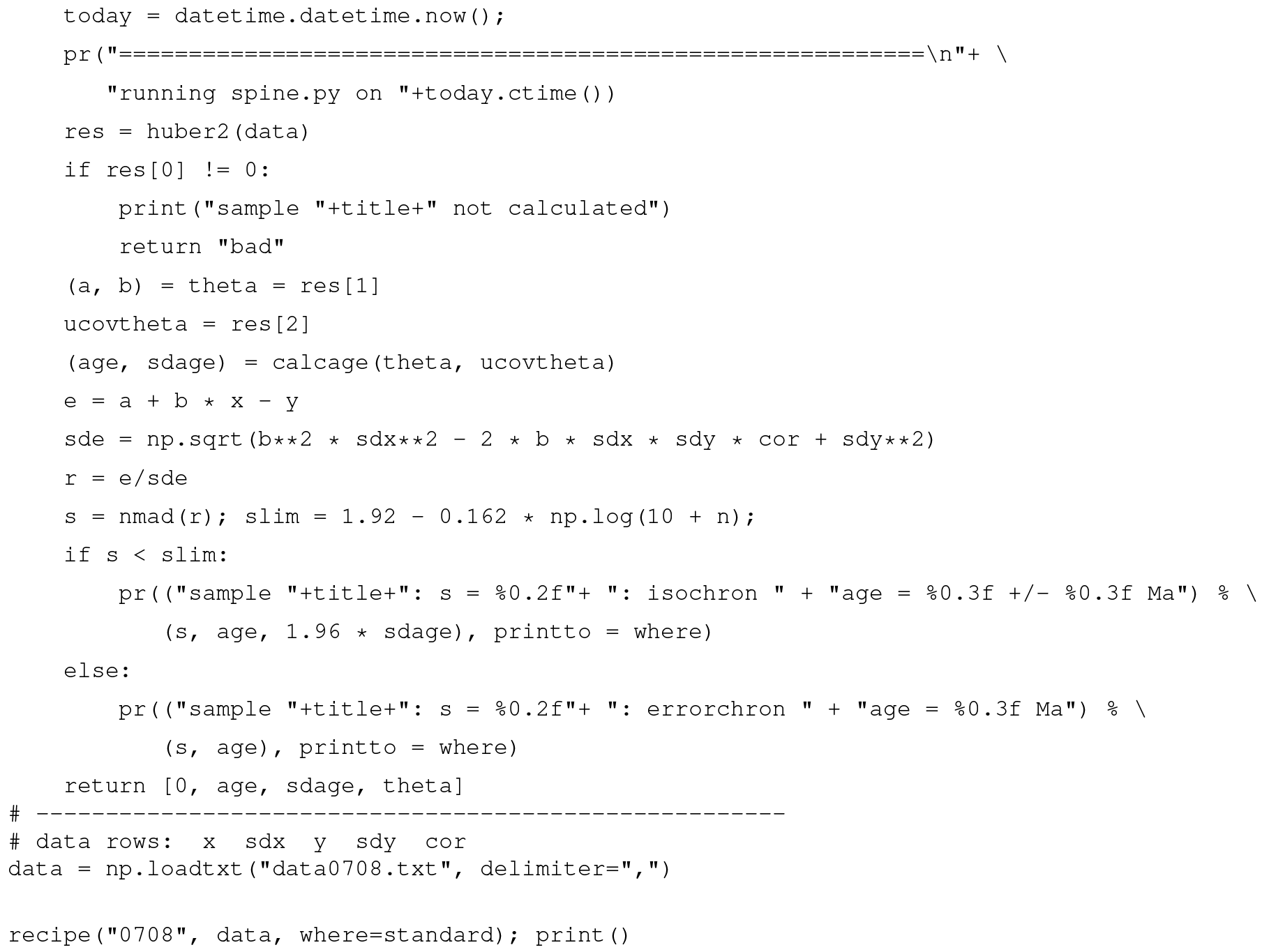
The second iteration in Appendix B is coded in the Python function, huber2. The starting point for the iteration is provided by the function, siegel (Siegel, 1982). The calling function, recipe, is a placeholder for a more general function to be written by the user.

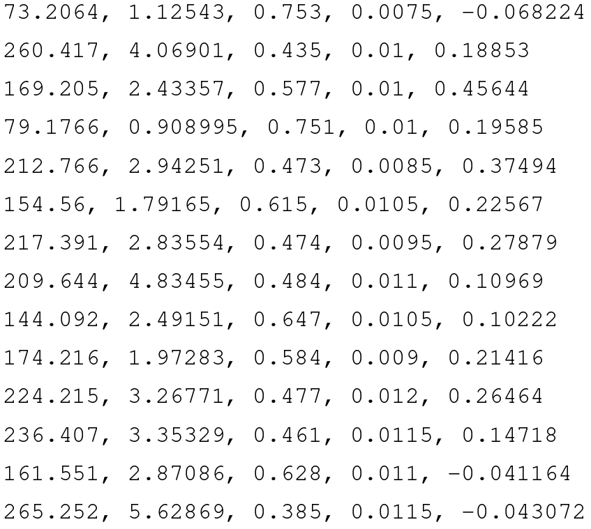
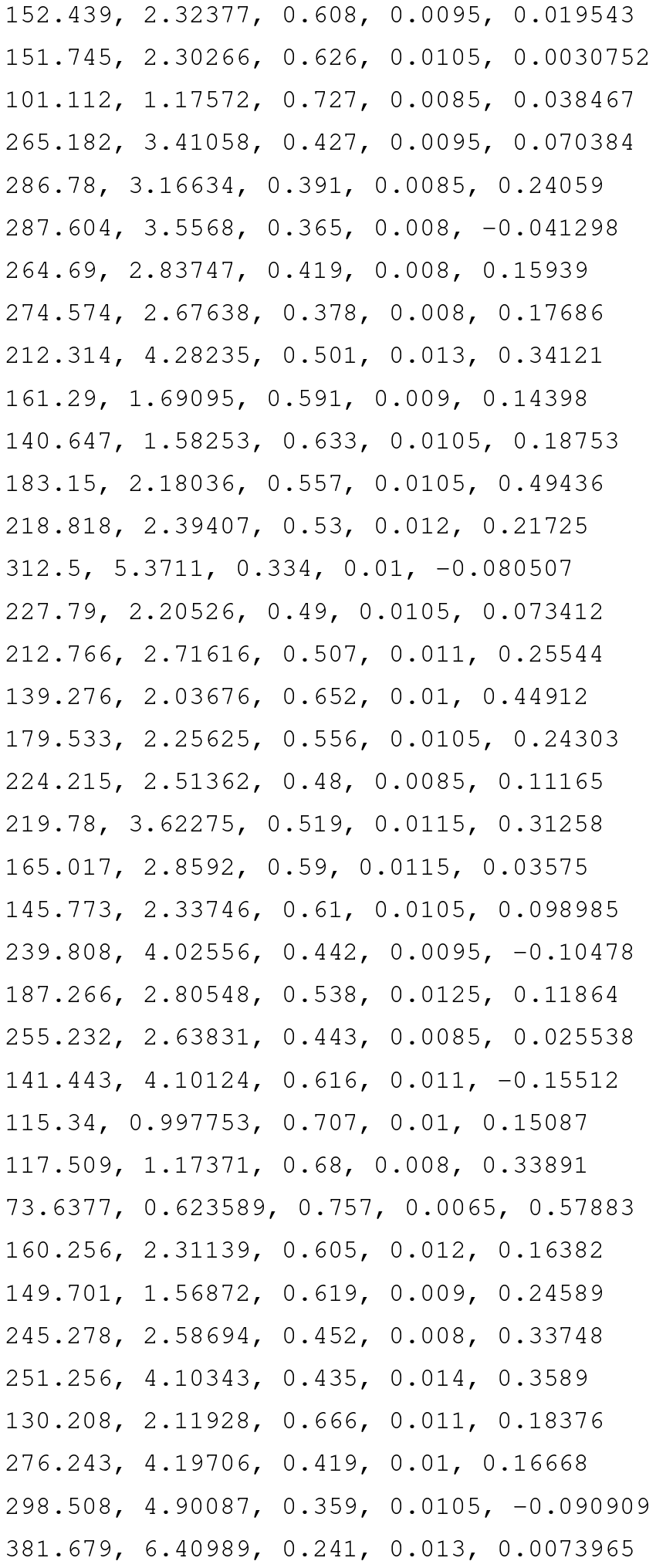
Datafile for sample 0708, data0708.txt, see Fig. 6

Example output, running on the command line

Appendix D: Simulation setup

This work was originally motivated by the dating of speleothems using the lower intercept with a U–Pb concordia in Tera–Wasserburg-style plots (Woodhead et al., 2012). This paper therefore discusses {x,y} data with the expectation that $x{=}^{\mathrm{238}}\mathrm{U}{/}^{\mathrm{206}}\mathrm{Pb}$ and $y{=}^{\mathrm{207}}\mathrm{Pb}{/}^{\mathrm{206}}\mathrm{Pb}$, but the logic and the algorithm are in no way restricted to this system.

Overall, 10 000 simulated datasets, each containing 5, 6, 8, 10, and 15 data points, respectively, were used to assess spine. Each dataset corresponds to an age of 4 Ma, with an underlying trend chosen to be $y=\mathrm{0.811}-\mathrm{0.000474737}x$. For each dataset, the x values were drawn from a uniform probability distribution with bounds {400,1100} (so the x values are not equally spaced). Data points are assigned uncertainty with ${\mathit{\sigma }}_{x_k}=\mathrm{0}$ and a fixed ${\mathit{\sigma }}_{y_k}=\mathrm{0.00125}$, the latter representing the analytical uncertainty, propagated from both the x and y measurements into y. In a real {²³⁸U∕²⁰⁶Pb, ²⁰⁷Pb∕²⁰⁶Pb} dataset, ${\mathit{\sigma }}_{x_k}$ and ${\mathit{\sigma }}_{y_k}$ would be finite and correlated. However, this makes no difference to the calculations once data are processed into r_k form as in Fig. 2. For a given dataset, scatter is introduced into the data by drawing the y values from an uncertainty distribution, centred on the underlying trend, that may be either Gaussian (N) or one of three contaminated Gaussian distributions – 5 %3N, 25 %5N, or 10 %10N – as in Powell et al. (2002). For n=10 and Gaussian-distributed uncertainties, the age uncertainty obtained is approximately σ_t=0.01 Ma.

Results are presented in terms of kernel density estimates using an Epanechnikov kernel (Wand and Jones, 1995). Kernel density estimates (kde) are a way of presenting data that could otherwise be plotted as a histogram, normally normalised so that – like a probability distribution – the area under the kde curve is 1. The smoothness of the kde is controlled by a smoothing constant whose value was chosen to be just large enough for the kde to appear smooth, given that 10 000 datasets are used in each kde.

Appendix E: spine handling outliers

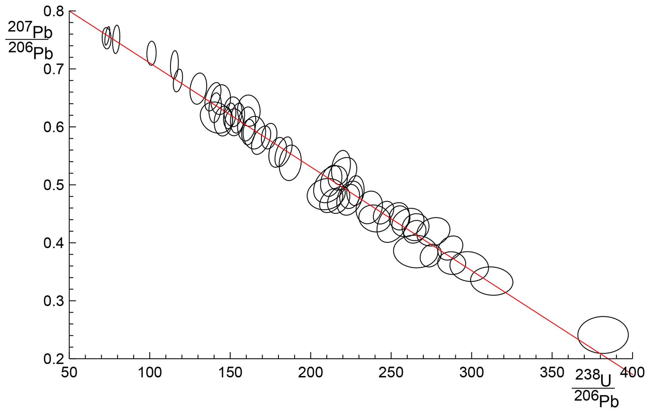
To see the consequence of outliers stemming from residuals from a contaminated Gaussian distribution, a dataset from simulations is shown in Fig. E1 and its corresponding quantile–quantile plot in Fig. E2. This simulation, with n=50 and 25 %3N and a true age of 4.00 Ma, follows the approach in Appendix D, but the uncertainty on the y values is taken to be an order of magnitude larger (to be comparable with sample 0708). The shape of Fig. E2 is typical of contaminated Gaussian distributions in samples of this size, with outliers lying outside the band between the dashed blue lines. The spine age is 3.95 Ma, whilst the york age is higher, 4.11 Ma, $\mathrm{\Delta }=+\mathrm{3.0}\mathit{\sigma }$ of the spine age, due to the effect of the outliers. Here, 𝚖𝚜𝚠𝚍=4.35, so isoplot would give a model 2 age, 4.19 Ma, with Δ=4.27, being more affected by the outliers than york.

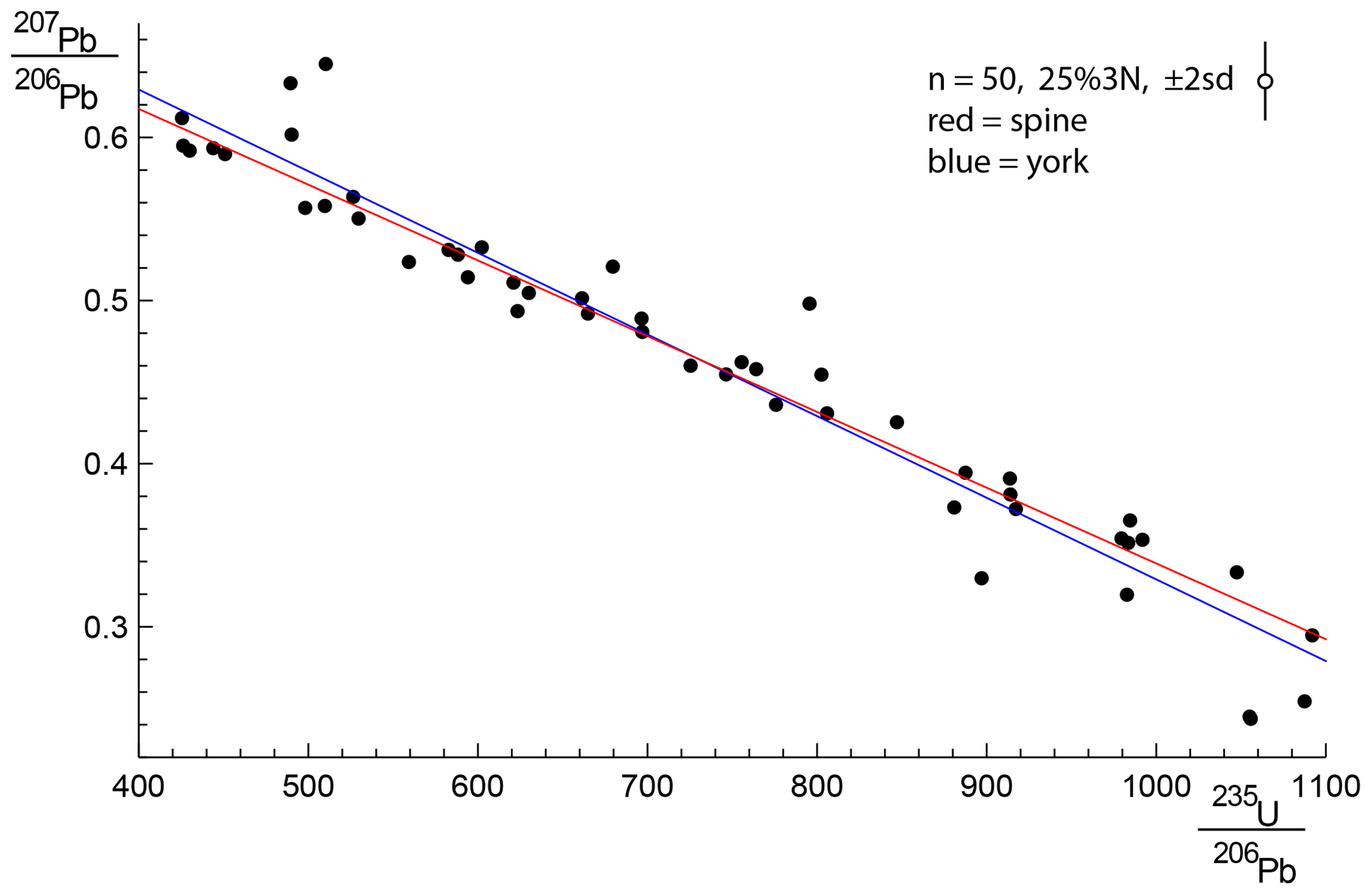
Figure E1 A 25 %3N simulation with n=50, with the spine fit in red and the york fit in blue. The 2σ uncertainty applied to the y value of each data point is indicated in the top right of the figure. See text.

Figure E2 Quantile–quantile plot, for example, in Fig. E1. See text.

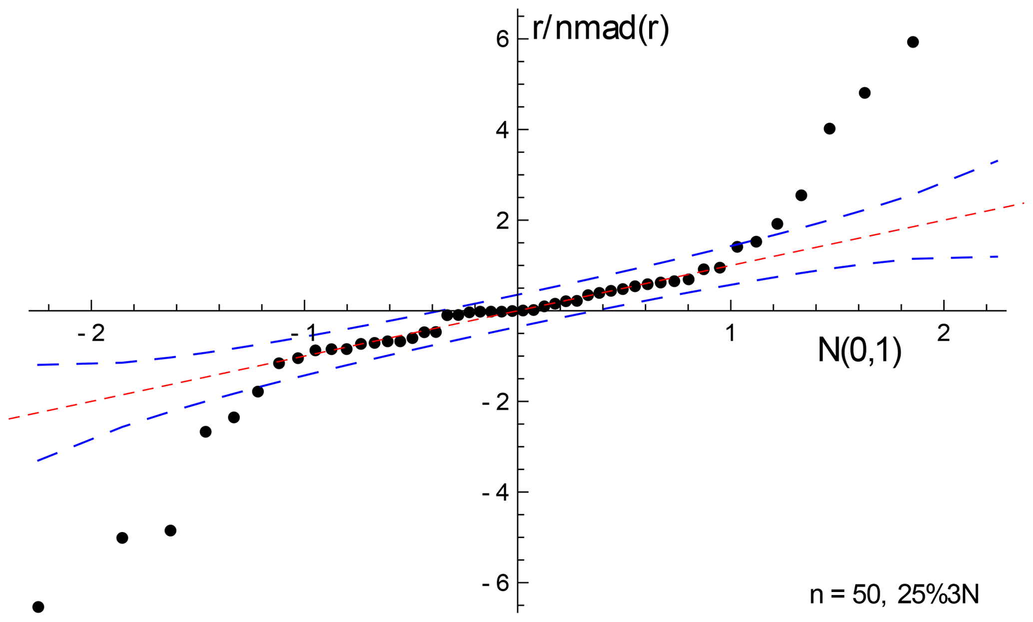
In general, with larger contaminated Gaussian datasets, the differences between the spine and york ages are not dramatic, even if there are obvious outliers in the quantile–quantile plots. In 10 000 simulated datasets with n=50 and 25 %3N, a 95 % confidence interval on Δ is ±1.5.