AI-Track-tive: open-source software for automated recognition and counting of surface semi-tracks using computer vision (artificial intelligence)

A new method for automatic counting of etched fission tracks in minerals is described and presented in this article. Artificial intelligence techniques such as deep neural networks and computer vision were trained to detect fission surface semi-tracks on images. The deep neural networks can be used in an open-source computer program for semi-automated fission track dating called “AI-Track-tive”. Our custom-trained deep neural networks use the YOLOv3 object detection algorithm, which is currently one of the most powerful and fastest object recognition algorithms. The developed program successfully finds most of the fission tracks in the microscope images; however, the user still needs to supervise the automatic counting. The presented deep neural networks have high precision for apatite (97 %) and mica (98 %). Recall values are lower for apatite (86 %) than for mica (91 %). The application can be used online at https://ai-track-tive.ugent.be (last access: 29 June 2021), or it can be downloaded as an offline application for Windows.

1 Introduction

Fission track dating is a low-temperature thermochronological dating technique applicable on several minerals. It was first described in glass by Fleischer and Price (1964) and in apatite by Naeser and Faul (1969). These findings were later summarized in the seminal book by Fleischer et al. (1975). Since the discovery of the potential of apatite fission track dating for reconstructing thermal histories (e.g. Gleadow et al., 1986; Green et al., 1986; Wagner, 1981), apatite fission track dating has been utilized in order to reconstruct thermal histories of basement rocks and apatite-bearing sedimentary rocks (e.g. Malusà and Fitzgerald, 2019; Wagner and Van den haute, 1992). As of 2020, more than 200 scientific papers with apatite fission track dating results are published every year. Hence, apatite fission track dating is currently a widely applied technique in tectonics and other studies.

Fission track dating techniques are labour-intensive and are highly dependent on accurate semi-track recognition using optical microscopy. Automation of the track identification process and counting could decrease the analysis time and increase reproducibility. Several attempts have been made to develop automatic counting techniques (e.g. Belloni et al., 2000; Gold et al., 1984; Kumar, 2015; Petford et al., 1993). The Melbourne Thermochronology Group in collaboration with Autoscan Systems Pty. Ltd. was the first to provide an automatic fission track counting system in combination with Zeiss microscopes. Currently, the only available automatic fission track recognition software package is called FastTracks. It is based on the patented technology of “coincidence mapping” (Gleadow et al., 2009). This procedure includes capturing microscopy images with both reflected and transmitted light; after applying a threshold to both images, a binary image is obtained. Fission tracks are automatically recognized where the binary image of the transmitted light source and reflected light source coincide (Gleadow et al., 2009). Recently, potential improvements for discriminating overlapping fission tracks have also been proposed (de Siqueira et al., 2019).

Despite promising initial tests and agreement between the manually and automatically counted fission track samples reported in Gleadow et al. (2009), challenges remain regarding the track detection strategy (Enkelmann et al., 2012). The automatic track detection technique from Gleadow et al. (2009) incorporated in earlier versions of FastTracks (Autoscan Systems Pty. Ltd.) did not work well in the case of (1) internal reflections (Gleadow et al., 2009), (2) surface relief (Gleadow et al., 2009), (3) over- or underexposed images (Gleadow et al., 2009), (4) shallow-dipping tracks (Gleadow et al., 2009), and (5) very short tracks with very short tails. More complex tests of the automatic counting software (FastTracks) undertaken by two analysts from the University of Tübingen (Germany) showed that automatic counting without manual review leads to severely inaccurate and dispersed counting results that are less efficient with respect to time than manual counting using the “sandwich technique” (Enkelmann et al., 2012). However, the creators are continuously developing the system and have solved the aforementioned problems. This has resulted in fission track analysis software that is utilized by most fission track labs, and this software is generally regarded as the one and only golden standard for automated fission track dating.

This paper presents a completely new approach regarding the automatic detection of fission tracks in both apatite and muscovite. Normally, fission tracks are detected using segmentation of the image into a binary image (Belloni et al., 2000; Gleadow et al., 2009; Gold et al., 1984; Petford et al., 1993). Here, in our approach, segmentation strategies are abandoned and are replaced by the development of computer vision (so-called deep neural networks – DNNs) capable of detecting hundreds of fission tracks in a 1000× magnification microscope image. Later in this paper, it will be shown that artificial intelligence techniques, such as computer vision, could replace labour-intensive manual counting, as already recognized by the pioneering work of Kumar (2015). Kumar (2015) was the first to successfully apply one machine learning technique (support vector machine) on a dataset of high-quality single (although this was not distinctly specified) semi-track images (30 µm × 30 µm). On the contrary, our paper presenting AI-Track-tive reports results of deep neural networks that can detect one to hundreds of semi-tracks in an individual 117.5 µm (width) × 117.5 µm (height) image. Our new potential solution for apatite fission track dating is currently available as an offline executable program for Windows (.exe) or online at https://ai-track-tive.ugent.be. The Python source code, deep neural networks, and the method to train a deep neural network are also available to the scientific community at https://github.com/SimonNachtergaele/AI-Track-tive (last access: 29 June 2021).

2 Methods

2.1 System requirements

AI-Track-tive uses two deep neural networks capable of detecting fission tracks in apatite and in muscovite mica. The deep neural networks have been trained on microscope images taken at 1000× magnification. Using deep neural networks, unanalysed images can be analysed automatically after which it is possible to apply manual corrections. Although it is tested on output from a Nikon Ni-E Eclipse microscope with Nikon–TRACKFlow software (Van Ranst et al., 2020), AI-Track-tive is certainly platform independent. The only required input for AI-Track-tive are .jpg microscopy images from both transmitted and reflected light with an appropriate size between 0.5 MP (megapixels) and 4 MP (e.g 1608 px × 1608 px or 804 px × 804 px). The offline windows application of AI-Track-tive contains a graphical user interface (GUI) and instructions window from which it is easy to choose the appropriate analysis settings and the specific images. The only requirements to train a custom-made DNN is a good internet connection and a Google account. The necessary steps to create a database with self-annotated images are specified on our website.

2.2 Development

The software makes use of a self-trained deep neural network based on the Darknet-53 “backbone” (Redmon and Farhadi, 2018), which has become extremely popular in object recognition for all kinds of object detection purposes. The Darknet-53 backbone and the YOLOv3 “head” configuration can be combined and trained to be used as an automatic object detection tool. This deep neural network can be trained to recognize multiple classes – for example, cats or dogs. The deep neural network presented in this paper is trained on only one class, i.e. etched semi-tracks. Two deep neural networks were trained specifically for detecting semi-tracks in apatite and in mica. They were both trained on a manually annotated dataset of 50 images for apatite and 50 images for mica.

The offline application “AI-Track-tive” (see Supplement) has been developed in Python v3.8 (Van Rossum and Drake, 1995) using several Python modules, such as an open-source computer vision module called OpenCV (Bradski, 2000). The offline application is constructed using Tkinter (Lundh, 1999). The online web application is constructed using the Python Flask web framework (Grinberg, 2018), JavaScript, and HTML 5.

2.2.1 Sample preparation

In order to create suitable images for DNN training, we converted the z-stacks (.nd2 files) acquired by the Nikon Ni-E Eclipse microscope to single-image 1608 px × 1608 px .tiff images using the NIS-Elements Advanced Research software package. It is assumed that the microscopy software rotates and horizontally flips the mica images before exporting them to .tiff files. Subsequently, we converted these images to “smaller” .jpg format using the Fiji freeware (Schindelin et al., 2012). In Fiji, we converted the .tiff images to .jpg using no compression, resulting in 1608 px × 1608 px images (2.59 MP). We then also implemented a 0.5 factor compression which resulted in smaller 804 px × 804 px .jpg images (0.64 MP). The training dataset consisted of images that were in focus and slightly out of focus.

2.2.2 Deep neural networks: introduction

Our deep neural network (DNN) consists of two parts: a backbone and a head which detects the object of interest. As mentioned, we opted for a Darknet-53 backbone (Redmon and Farhadi, 2018) combined with a YOLOv3 head (Redmon and Farhadi, 2018). The Darknet-53 backbone consists of 53 convolutional layers and some residual layers in between (Redmon and Farhadi, 2018). The Darknet-53 backbone in combination with a YOLOv3 head can be trained so that it recognizes an object of choice. The training process is a computationally demanding process, requiring the force of high-end graphics processing units (GPUs), that would take several days on normal computers. In order to shorten this training process, it is possible to use powerful GPU units from Google Colab. Utilizing the hosted runtime from Google, it is possible to use the available high-end GPUs for several hours while executing a Jupyter Notebook.

While many other alternatives are available, we chose YOLOv3 with a Darknet-53 pre-trained model, as it is freely available and is currently one of the fastest and most accurate convolutional neural networks (Redmon and Farhadi, 2018). Using YOLOv3, it is possible to perform real-life object detection using a live camera or live computer screen (Redmon and Farhadi, 2018). From a geologist's perspective it seems that object detection using artificial intelligence is a very rapidly evolving field in which several new DNN configurations are created every year (e.g. YOLOv4 in 2020). The chances are high that the presented YOLOv3 DNN could already be outdated in a few years. Therefore, we will provide all of the necessary steps to train a DNN that could potentially be more efficient than our current DNN. For these future DNNs, it should be possible to use AI-Track-tive with DNNs other than YOLO with the application of minor adaptations. OpenCV 4.5 can handle DNNs other than YOLO – for example, Caffe (Jia et al., 2014), Google's TensorFlow (Abadi et al., 2016), Facebook's Torch (Collobert et al., 2002), DLDT Openvino (https://software.intel.com/openvino-toolkit, last access: 29 June 2021), and ONNX (https://onnx.ai/, last access: 29 June 2021).

2.2.3 Deep neural networks: training and configuration

DNN training includes two steps. The first step involves annotating images with LabelImg (https://github.com/tzutalin/labelImg, last access: 29 June 2021) or AI-Track-tive. These training images were taken with transmitted light (using a Nikon Ni-E Eclipse optical light microscope at 1000× magnification) and were square-sized colour images with a width and height of 117.5 µm. This first step includes manually drawing thousands of rectangles covering every semi-track. It is advisable to train the DNN on a dataset in which several tracks are overlapping with one another, the light exposure varies, and the images are slightly out of focus and in focus. For apatite, we drew a total of 4734 rectangles, indicating 4734 semi-tracks in 50 images. For mica, a total of 6212 semi-tracks were added in 50 images. The arithmetic mean of track densities was, in this case, 7.9×10⁵ tracks cm⁻² (Fig. 1).

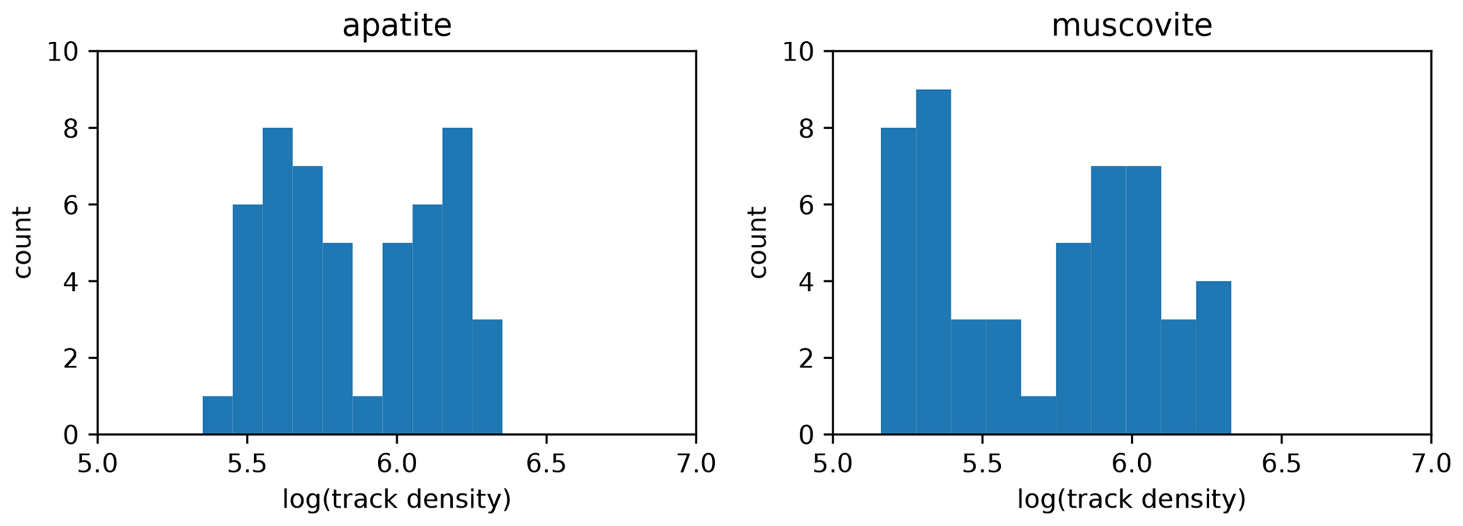
Figure 1 Frequency histograms illustrating the areal track density of the training datasets. The horizontal axis expresses the 10-based log of the areal track density of the training dataset.

The second step is executing a Jupyter Notebook and connecting it to Google Colab (https://colab.research.google.com, last access: 29 June 2021). Google Colab is a free platform where one can execute their Python code using Google's graphics processing unit (GPU) resources. This resource provides the possibility to train a DNN in a few hours using much more GPU power than is normally available. Google Colab provides a maximum of 8 h of working time using very powerful (but expensive) GPUs such as NVIDIA Tesla K8, T4, P4, or P100. These GPUs are utilized to adapt the Darknet53 (.weights) file to the training dataset using a configuration file (.cfg) through an iterative training process during which it will progressively recognize the tracks more successfully. This iterative training process creates a new .weights file for every 100 iterations. Every training iteration gives a misfit value, called the “average loss”. The average loss is a value that expresses the accuracy of track recognition of the trained .weights file. This average loss value is high at the beginning of the training process (∼ 10³) but decreases to < 10 after a few hours of training. The speed of the iterative training process depends on many factors that are specified in the YOLOv3 head. It is possible to change the training process by adapting the configuration of the YOLOv3 head in the .cfg file. In the .cfg file, several configuration parameters of the DNN are specified such as the learning rate and network size. In our case, the network size is was 416 × 416, implying that it will resize our 804 px × 804 px images to 416 × 416. We experienced that increasing the network size from 416 × 416 to 608 × 608 or increasing the image size from 804 px × 804 px to 1608 px × 1608 px strongly decreased the iteration speed. Hence, we chose to train a DNN with a 416 × 416 network size using 804 px × 804 px images.

2.2.4 Deep neural networks: testing

The efficiency of every trained DNN can be tested using images (“test images”) that are not part of the training dataset. When the YOLOv3 configuration is used to find the object of interest (semi-tracks), it predicts a high number of bounding boxes with each having a different place, width, height, and confidence value in the image. The confidence value is normally high (> 95 %) for the easily recognized tracks and rather low for the less obvious semi-tracks, as illustrated in Fig. 2. A user-defined threshold value defines the value (e.g. 50 %) above which rectangles are drawn on the test image.

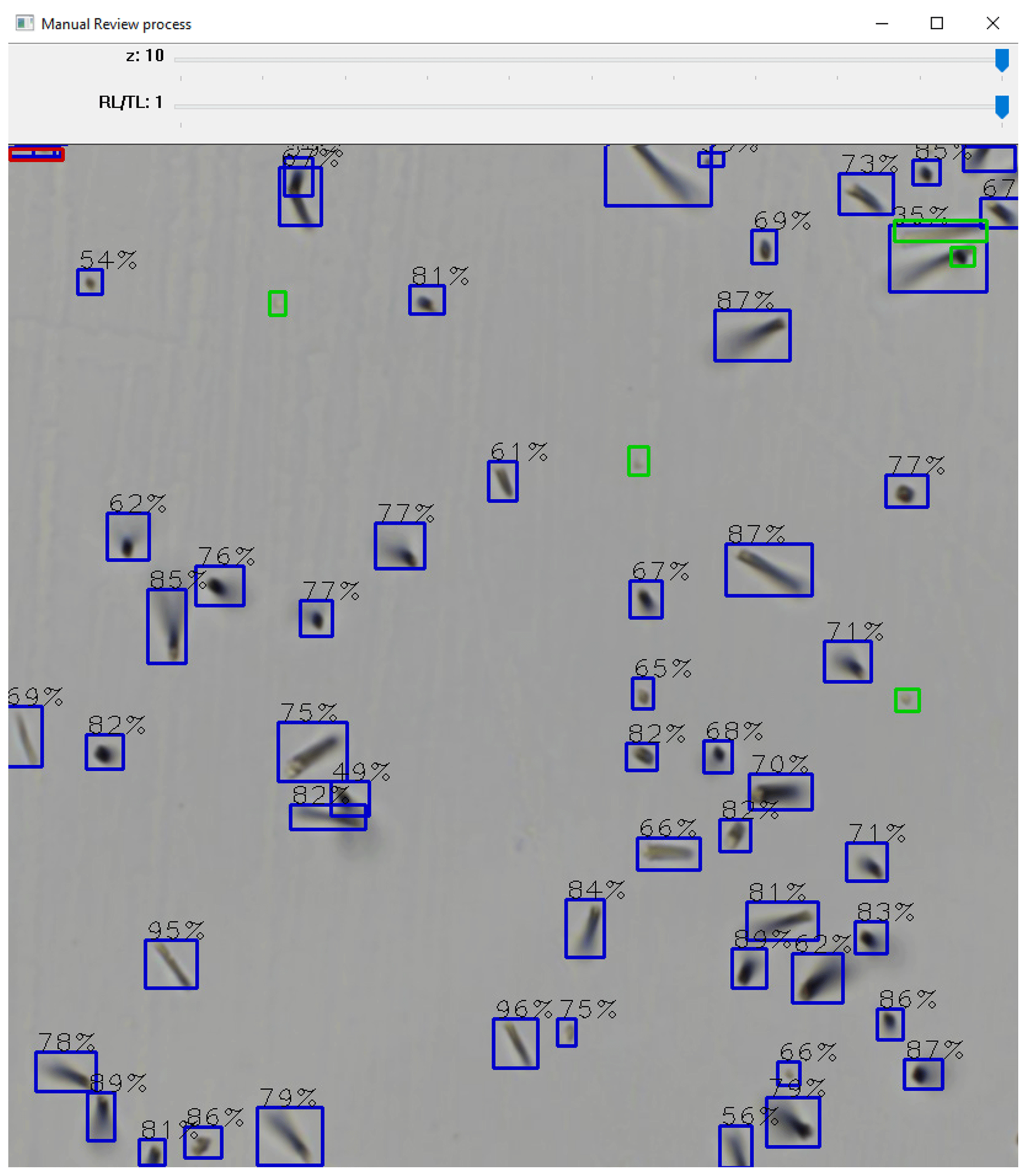
Figure 2 Fission track recognition in muscovite (external detector). Blue squares indicate automatically recognized semi-tracks. The percentage displayed above every blue box indicates the confidence score for that particular group of pixels to be recognized as a semi-track. The small fraction of unrecognized tracks (“false negatives”) is manually indicated using green squares. Red squares indicate erroneously indicated tracks (“false positives”). The two track bars above the image indicate the possibility of comparing different focal levels or change between reflected and transmitted light.

For one semi-track, YOLOv3 predicts several overlapping bounding boxes (Redmon et al., 2016). Therefore, an essential non-maximum suppression step leads to one rectangle surrounding the semi-track. In the commonly occurring scenario that several semi-tracks coincide or overlap, it is highly likely that only one rectangle is drawn after conservative non-maximum suppression filtering. AI-Track-tive sometimes struggles to identify multiple tracks, even though we adapted the “nms_treshold” value in order to allow the drawing of multiple boxes in the case of coinciding semi-tracks.

3 Results

3.1 AI-Track-tive: new open-source software for semi-automatic fission track dating

The result of the unique strategy for automated fission track identification is embedded in AI-Track-tive. AI-Track-tive is available in two forms: one offline and one online application. The downloadable offline application is typically for Windows users and requires installation on a pc/laptop. The online application does not require any installation and is hosted at http://ai-track-tive.ugent.be. The web app has been successfully tested on Google Chrome and Mozilla Firefox. The online app does not allow automatic etch pit size determination or live track recognition. The core of AI-track-tive, i.e. fission track counting, is possible using both the on- and offline application.

Currently, AI-Track-tive is developed for apatite and external detector (mica). The user can import one or two transmitted light images with different z levels in AI-Track-tive; from this input, the software will create a blended image through which the focal level can be changed manually. In this fashion, the analyst gets a 3D impression of the image containing the tracks. The user also has the ability to import reflected light images and change between the transmitted light and reflected light images rapidly using the computer mouse wheel function.

The user can optionally choose for a region of interest in which the fission tracks will be sought as well as between the different options with different sizes. When all settings are filled in and all images are uploaded, AI-Track-tive finds and annotates the detected fission tracks in less than a few seconds. Due to the very rapid YOLOv3 algorithm (Redmon et al., 2016; Redmon and Farhadi, 2018), it is possible to instantaneously detect the semi-tracks in the loaded images. The result of the track recognition is an image in which every detected fission track is indicated with a rectangle comprising the detected fission track. Every track associated with a rectangle that is located with more than half of its area inside the region of interest is counted. Each track has a certain confidence score, as illustrated in Fig. 2. This confidence score is close to one for easily recognizable tracks and much lower for overlapping tracks. The confidence score is shown in Fig. 2 for the sake of illustration but is normally it is not displayed. Currently, track detection is not 100 % successful for every image; therefore, manual review is absolutely necessary and essential to obtain useful data. While reviewing the track detection results, it is possible to switch between reflected and transmitted light images. Unidentified semi-tracks can be manually added, and mistakenly added tracks can be removed using the computer mouse buttons following the instructions. These manual corrections will be immediately displayed on the microscope image using a different colour . The manual corrections that each user carries out on the website will be saved in our database. These data can be used later as a potential dataset for DNN training.

The adjusted image is saved as a .png or .jpg file after the manual revision process is completed. Track counting results are exported in .csv files along with all useful information. Hence, performing your own ζ calibration (Hurford and Green, 1983) or GQR calibration (Jonckheere, 2003) is possible.

3.1.1 AI-Track-tive: live fission track recognition

Due to the accurate and fast nature of the YOLOv3 object detection algorithm, it is possible to do real-time object detection (Redmon and Farhadi, 2018). This real-time track detection is only available in the offline application due to the lack of GPU power on our server. In the offline, downloadable application of AI-Track-tive, it is possible to let a DNN detect fission tracks on live images from your computer screen. The only drawback for the “live fission track recognition” is the computer processing time of approximately 0.3 to 0.5 s, depending on computer system hardware. Real-time object-detecting neural networks are much more useful in environments in which the detected objects are dynamic. Obviously, etched semi-tracks are static, so it is not as helpful to detect fission tracks on live images. The usefulness of this “live recognition” function might be twofold: the first application lies in the fast evaluation of the trained deep neural networks; the second potential application relates to an implementation into microscope software. “Smart” microscopes using live semi-track recognition could distinguish apatite (containing semi-tracks) from other minerals that are in between the apatite grains.

3.1.2 AI-Track-tive: DNN training

It is possible to use AI-Track-tive to construct a training dataset for further DNN training based on a custom dataset. This training dataset can be created by loading transmitted light images in AI-Track-tive and highlighting the tracks manually. In this fashion, an unexperienced programmer could use this software instead of other dedicated (and more widely tested) software (LabelImg) to create a training dataset comprising images (.jpg) and accompanying annotations (.txt) files.

In the online application, it is possible to fill in details of the optical microscope on which you collected the images. These manual track annotation measurements will be downloaded in the client's browser and also stored in a database containing all image parameters and files.

3.1.3 AI-Track-tive: etch pit diameter size (D_par) measurement

The offline application of AI-Track-tive also allows the user to determine the D_par value (Donelick, 1993), which is the size of the semi-track's etch pits measured in the c-axis direction (Fig. 3). For this step, AI-Track-tive does not use DNNs (yet); instead, it uses colour thresholding. Colour thresholding is the most commonly used technique for image segmentation. This colour thresholding is sensitive to unequal light exposure, although this is more or less solved by gamma correction. AI-Track-tive filters the D_par values using a threshold based on the minimum and maximum size of the etch pits. After the size discrimination step, AI-Track-tive uses another two filters based on the elongation factor (width-to-height ratio) and the directions (or angles) of the etch pits. The threshold values for these filters can be changed when advancing through the GUI.

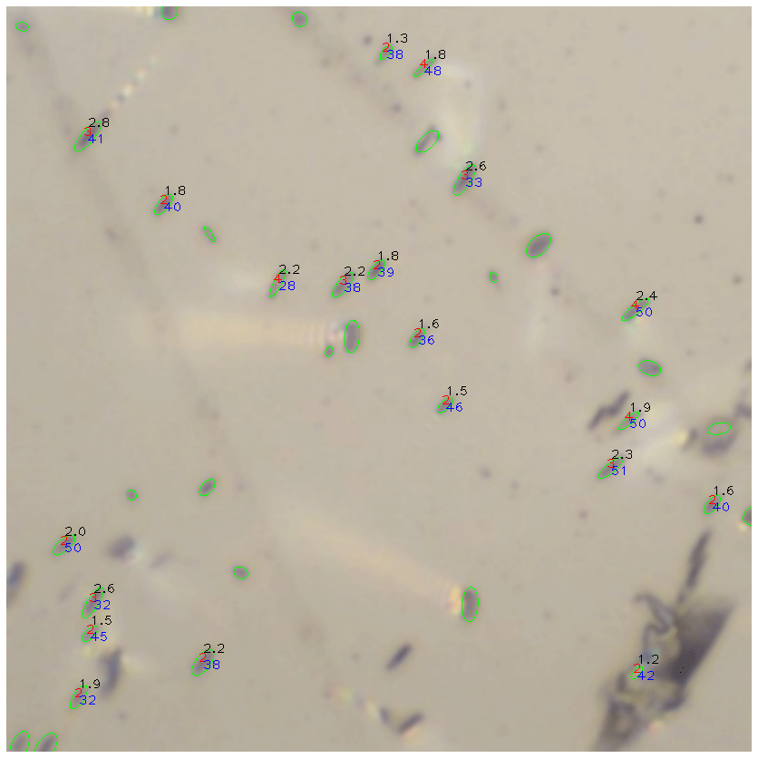
Figure 3 An example of a semi-automatic D_par measurement result obtained on a part of an image taken at 1000× magnification. The green ellipses are the remainders of a segmentation process. The values written next to the ellipses stand for the length in micrometres (black), the elongation factor (red), and the angle (blue). Some green ellipses show no values because they have been excluded by the elongation filter, direction filter, minimum size filter, or maximum size filter.

3.2 Semi-track detection efficiency

A series of analyses were undertaken in order to evaluate the efficiency of the semi-track identification in apatite and mica. Several apatite and mica samples with varying areal fission track densities were analysed. The efficiency tests were performed on 50 mica and 50 apatite images that were not included in the training dataset for the DNN development (Fig. 4). For almost all images, we opted to use a 100 µm × 100 µm square-shaped region of interest with tens or even hundreds of tracks in the image (Tables 1, 2). Apatite grains with varying uranium zoning and spontaneous track densities were analysed. The results of these experiments are listed in Table 1 (apatite) and Table 2 (mica). Widely used metrics for evaluating object recognition success are calculated using the correctly recognized semi-tracks (true positives – TP), unrecognized semi-tracks (false negatives – FN), and mistakenly recognized semi-tracks (false positives – FP). Typical metrics to evaluate the performance of object detection software are precision $\left(\frac{\mathrm{TP}}{\mathrm{TP}+\mathrm{FP}}\right)$ and recall (the true positivity rate, $\left(\frac{\mathrm{TP}}{\mathrm{TP}+\mathrm{FN}}\right)$).

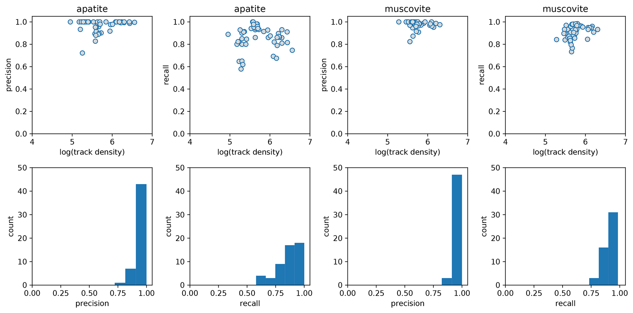
Figure 4 Performance metrics of the deep neural networks obtained on a dataset containing 50 “test images”. The precision (true positives $/$ (true positives + false positives)) and recall (true positives $/$ (true positives + false negatives)) of the automatic fission track recognition deep neural network are shown for apatite and muscovite mica (external detector). The 10-based log of areal track density (tracks cm⁻²) is shown on the horizontal axis of the upper scatter plots. The frequency histograms below show the distribution of the performance metrics.

Table 1 Test results of the automatic fission track recognition in apatite (confidence threshold = 0.1). Areal track density is expressed in tracks per square centimetre (tracks cm⁻²). The number of correctly automatically detected tracks (true positives), manually detected tracks (false negatives), and erroneously detected tracks (false positives) are indicated by n_auto, n_manual, and n_auto false respectively.

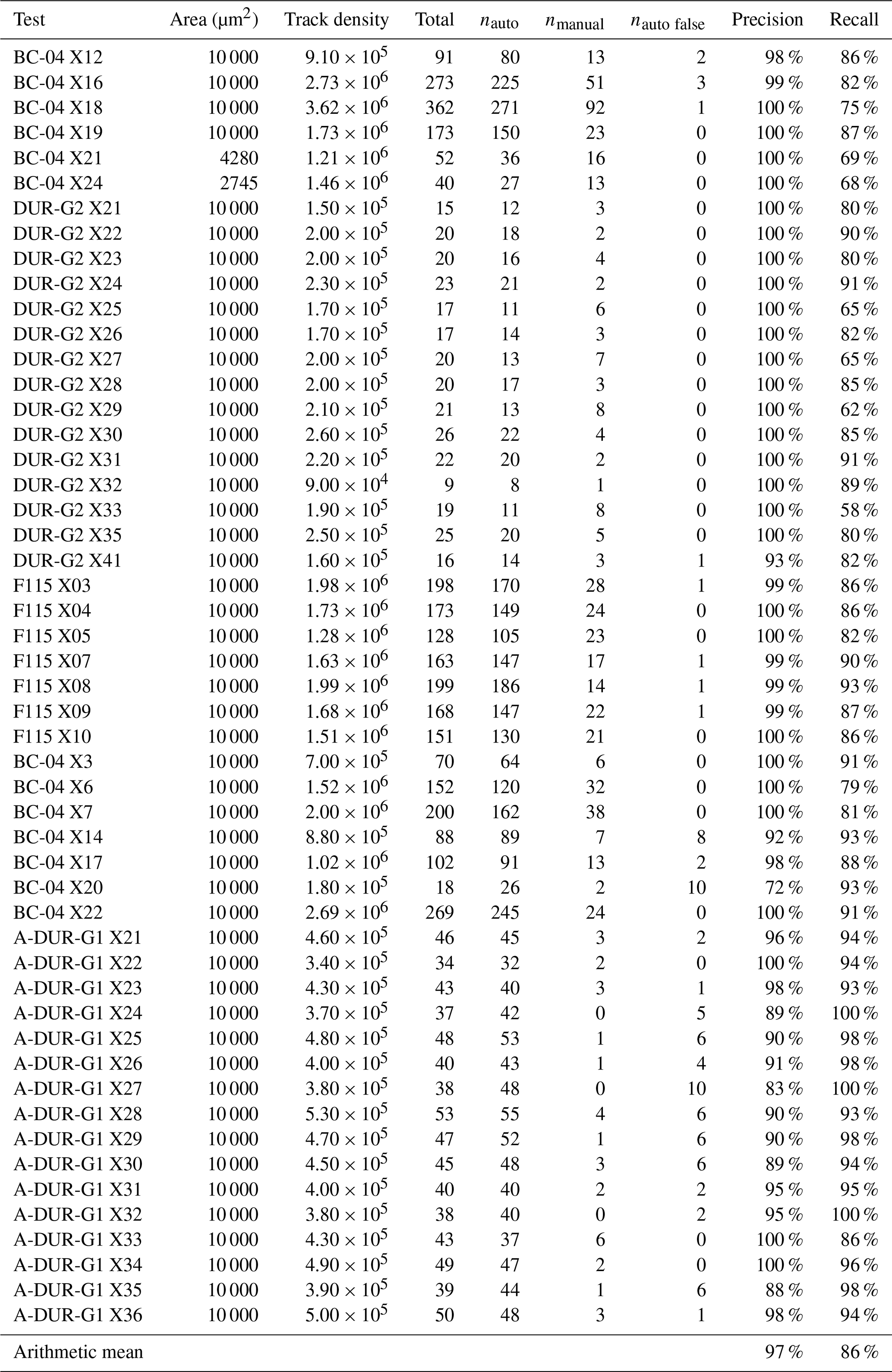
Table 2 Test results of the automatic fission track recognition in muscovite mica (confidence threshold = 0.3). Areal track density is expressed in tracks per square centimetre (tracks cm⁻²). The number of correctly automatically detected tracks (true positives), manually detected tracks (false negatives), and erroneously detected tracks (false positives) are indicated by n_auto, n_manual, and n_auto false respectively.

3.2.1 Apatite

For the apatite images from our test dataset, the arithmetic mean of the precision equals 97 %, whereas the recall is 86 %. The precision is very high and indicates that very few false positives are found. A precision lower than 0.8 only occurs for very low track densities, which is probably due to the fact that a few false positives have a relatively high impact in an image where only 20 tracks are supposed to be recognized. The true positivity rate (recall) value is 86 %, which is lower than the average precision. Despite the overall high scores for recall (Fig. 4), it sometimes occurs that recall is lower than 0.8. Hence, it is essential that the unrecognized tracks (false negatives) are manually added.

3.2.2 External detector

For the muscovite images from our test dataset, the arithmetic mean of the precision equals 98 % compared to a recall of 91 %. These metrics are both higher than those obtained for apatite. The precision is very high (close to 100 %), indicating that false positives are scarce. Recall is above 90 % and only drops below 80 % for a handful of samples with low track densities (Fig. 4). The frequency histogram of the recall values and precision values are less skewed compared with the histograms of apatite (Fig. 4).

3.3 Analysis time

One small experiment was undertaken in which fission tracks were counted in both apatite and external detector. The results of these experiments are summarized in Table 3 and are compared to previous results using FastTracks reported in Enkelmann et al. (2012) as well as more up-to-date values of FastTracks (Andrew Gleadow, personal communication, 2020). For our time analysis experiment, 25 coordinates in a pre-annealed Durango sample (A-DUR) and its external mica detector were analysed by Simon Nachtergaele. Selecting and imaging 25 locations in the Durango sample and its external detector took 25–35 min using Nikon–TRACKFlow (Van Ranst et al., 2020). Counting fission tracks in 25 locations in one pre-annealed and irradiated Durango sample and its external detector (including manual reviewing) using AI-Track-tive took 30 min in total, but it is expected that it would take longer for samples with higher track densities (e.g. 60 min). A full, independent, comparison between existing software packages and the software presented in this study lies outside the scope of this paper.

Table 3 Estimated time for 20–30 grains/polygons using different automated track recognition software packages and manual counting results from Enkelmann et al. (2012). Non-specified information is indicated using “ns”.

4 Discussion

4.1 Automatic semi-track recognition

The success rate of automatic track recognition has been tested for several (∼ 50) different images of apatite and external detector (mica) images. The automatic track recognition results show that the computer vision strategy is (currently) not detecting all semi-tracks in apatite (Table 1) and mica (Table 2). Hence, manually reviewing the results and indicating the “missed” tracks (false negatives) is essential.

The precision and recall of both the apatite and mica fission track deep neural networks is compared to the areal track densities in the scatter plots shown in Fig. 4. The upper limit of 10⁷ tracks cm⁻² was defined for fission track identification using optical microscopy (Wagner, 1978). The lower limit of 10⁴ tracks cm⁻² was chosen arbitrarily based on the fact that apatite fission track samples in most studies have track densities within the range of 10⁵ to 10⁷ tracks cm⁻². For track densities between 10³ and 10⁵ tracks cm⁻², it is still possible to apply fission track analysis, but it is more time-consuming with respect to sample scanning and image acquisition (i.e. finding a statistically adequate number of countable tracks in large surface areas and/or a high number of individual apatite grains). However, apatite with very low track densities of 10³ to 10⁴ tracks cm⁻² extracted from low-uranium lithologies were successfully analysed (Ansberque et al., 2021), although they were not part of the testing dataset.

The precision and recall values discussed earlier are high and indicate that the large majority of the semi-tracks can be detected in all images from our test dataset. However, coinciding semi-tracks are difficult to detect for both humans and deep neural networks. Therefore, the deep neural networks were trained on 50 images (Table 1) in which the track densities were high and the individual tracks were sometimes hard to identify due to spatial overlap (Fig. 1).

4.2 Current state and outlook

With the development of AI-Track-tive, it was possible to successfully introduce artificial intelligence techniques (i.e. computer vision) into fission track dating. The program presented here has a comparable analysis speed to other automatic fission track recognition software, such as FastTracks from Autoscan Systems Pty. Ltd. (Table 3). Based on the current success rate of the program's track detection, we already think that a significant gain has been made. However, manually reviewing the automatic track recognition results is still (and will perhaps always be) necessary. The online web application saves all uploaded pictures, including all manual annotations made by the user. In the online app, it is also possible to provide the microscope type as extra information. All of the data (e.g. pictures, rectangles, and other info) that are uploaded by the users of the online AI-Track-tive application will be stored in a database when executing the application. These data could be used to make other deep neural networks for other minerals, microscopes, or etching protocols.

In the near future, it seems likely that computer power and artificial intelligence techniques will inevitably improve. Therefore, smarter deep neural networks with higher precision and recall values will likely be developed in the (near) future. Although we only worked with YOLOv3 algorithms (Redmon and Farhadi, 2018), we expect that other deep neural networks could also be used in AI-Track-tive. AI-Track-tive is an open-source initiative without any commercial purpose. The offline application is written entirely in Python, a popular programming language for scientists, so that it can be continuously developed by other scientists in the future. The back end of the online application is written using Python's Flask micro web framework. The front end of the online application is written in standard programming languages (JavaScript and HTML 5). We would appreciate voluntarily bug reporting to the developers. Future software updates will be announced on https://github.com/SimonNachtergaele/AI-Track-tive and on the https://ai-track-tive.ugent.be website.

5 Conclusions

In this paper, we presented a free method to train deep neural networks capable of detecting fission tracks using any type of microscope. We also introduced an open-source Python-based software called “AI-Track-tive” with which the trained neural networks can be tested. These neural networks can be tested on either acquired images (split z-stacks) or live images from the microscope camera. It is possible to use AI-Track-tive for apatite fission track dating of samples and/or standards. Finally, we provided our two deep neural networks and their training dataset, which is calibrated or trained on a Nikon Ni-E Eclipse set-up.

In summary, AI-Track-tive is

• available from https://ai-track-tive.ugent.be;

• unique because it is, to our knowledge, the first geological dating procedure using artificial intelligence;

• makes use of artificial intelligence (deep neural networks) in order to detect fission tracks automatically;

• capable of successfully finding almost all fission tracks in a sample, and unrecognized tracks can be manually added in an interactive window;

• reliable because it is not really sensitive to changes in optical settings, unlike a human operator;

• robust because the fission track detection criteria do not change with time, unlike a human operator;

• oriented toward the future, as it is software in which other, potentially smarter, deep neural networks can be implemented;

• open source in order to give all scientists the opportunity to improve their software for free through time – for this, we depend on the voluntary help of the fission track community to debug the software;

• tied to a database where all uploaded photos and information are stored. The uploaded data can be used in the development of other, potentially smarter, deep neural networks for apatite, mica, or other minerals.