How many grains are needed for quantifying catchment erosion from tracer thermochronology?

Detrital tracer thermochronology utilizes the relationship between bedrock thermochronometric age–elevation profiles and a distribution of detrital grain ages collected from riverine, glacial, or other sediment to study spatial variations in the distribution of catchment erosion. If bedrock ages increase linearly with elevation, spatially uniform erosion is expected to yield a detrital age distribution that mimics the shape of a catchment's hypsometric curve. Alternatively, a mismatch between detrital and hypsometric distributions may indicate spatial variability of sediment production within the source area. For studies seeking to identify the pattern of sediment production, detrital samples rarely exceed 100 grains due to the time and costs related to individual measurements. With sample sizes of this order, detecting the dissimilarity between two detrital age distributions produced by different catchment erosion scenarios can be difficult at a high statistical confidence level. However, there are no established software tools to quantify the uncertainty inherent to detrital tracer thermochronology as a function of sample size and spatial pattern of sediment production. As a result, practitioners are often left wondering “how many grains is enough to detect a certain signal?”. Here, we investigate how sample size affects the uncertainty of detrital age distributions and how such uncertainty affects the ability to infer a pattern of sediment production of the upstream area. We do this using the Kolmogorov–Smirnov statistic as a metric of dissimilarity among distributions. From this, we perform statistical hypothesis testing by means of Monte Carlo sampling. These techniques are implemented in a new tool (ESD_thermotrace) to (i) consistently report the confidence level allowed by the sample size as a function of application-specific variables and given a set of user-defined hypothetical erosion scenarios, (ii) analyze the statistical power to discern each scenario from the uniform erosion hypothesis, and (iii) identify the erosion scenario that is least dissimilar to the observed detrital sample (if available). ESD_thermotrace is made available as a new open-source Python-based script alongside the test data. Testing between different hypothesized erosion scenarios with this tool provides thermochronologists with the minimum sample size (i.e., number of bedrock and detrital grain ages) required to answer their specific scientific question at their desired level of statistical confidence.

1 Introduction

Tracer thermochronology uses the distribution of single-grain thermochronometric ages from detritus to infer the spatial pattern of erosion in the source area (e.g., Stock et al., 2006; Vermeesch, 2007). This approach is typically applied where bedrock thermochronometric age data exhibit a clear age–elevation relationship, allowing inference of the relative contribution of source elevations from the detrital grain age distribution. A detrital grain age distribution that closely follows the catchment's hypsometric curve (i.e., the cumulative distribution function of elevation area) is generally interpreted as indicative for spatially uniform erosion. Conversely, a detrital age distribution skewed towards younger (or older) ages may be the consequence of focused erosion at lower (or higher) elevations (Brewer et al., 2003). Tracer thermochronology has been shown to be a powerful tool to investigate the sub-catchment-scale variability of denudation. Geomorphologists have been able to infer changes in climatic parameters (Nibourel et al., 2015; Riebe et al., 2015), glacial erosional processes (Ehlers et al., 2015; Enkelmann and Ehlers, 2015; Clinger et al., 2020), sediment dynamics (Lang et al., 2018), relief evolution (McPhillips and Brandon, 2010; Whipp et al., 2009), occurrence of mass-wasting (Vermeesch, 2007; Whipp and Ehlers, 2019), and differences in rock uplift (McPhillips and Brandon, 2010; Glotzbach et al., 2013, 2018; Brewer et al., 2003; Ruhl and Hodges, 2005). Other work has noted that neglecting mineral fertility variations with catchment lithologies may challenge the conclusions of some of these studies (Malusà et al., 2016). Unfortunately, the number of measured detrital ages for tracer thermochronology is often dictated by inherent limitations of the sampled material and/or by available finances, rather than a science-based choice. Detrital sample sizes often range between 40 and 120 grains (e.g., Stock et al., 2006; Vermeesch, 2007; McPhillips and Brandon, 2010; Ehlers et al., 2015; Riebe et al., 2015; Glotzbach et al., 2018; Lang et al., 2018; Clinger et al., 2020) and are considered to yield high-confidence results when surpassing ∼100 grains based on previous work on sediment provenance analysis (Vermeesch, 2004). However, in unfortunate cases, two measured distributions generated from different erosional patterns cannot be statistically discerned at a high confidence level even with more than 100 grains. Although this issue has been well-known to the community (e.g., Avdeev et al., 2011) since the early days of such detrital studies (Brewer et al., 2003), there is no established tool to quantify the uncertainty inherent to detrital tracer thermochronology as a function of sample size and upstream pattern of sediment production. Moreover, the number of measured grains may often be based on convenience and/or habit.

Here, we complement previous work by investigating how sample size affects the uncertainty of detrital cooling age distributions and the related confidence in addressing the pattern of sediment production in the upstream area. We discuss the approaches used in previous case studies, upon which we develop a tool (Earth system dynamics – ESD_thermotrace) to consistently report confidence levels as a function of sample size and case-specific variables. We illustrate our approach using a published dataset from the Sierra Nevada, California (Stock et al., 2006). The proposed tool is made available as a new open-source Python-based script alongside the test data. We demonstrate how ESD_thermotrace can assist future tracer thermochronology studies in defining the necessary sample size to answer their specific scientific question. In cases where larger sample sizes are impossible to achieve, the statistical power of a tracer thermochronology analysis can be studied using our script.

2 Background information

Single-grain detrital age distributions are extensively applied in classical detrital geochronology studies (Hurford and Carter, 1991), where $\mathrm{U}/\mathrm{Pb}$ crystallization ages of zircon constitute by far the most used tool (Spiegel et al., 2004; Andersen, 2005; Malusà et al., 2013). In this type of application, the aim is to obtain the spectrum of all age components (i.e., age peaks) that characterize a siliciclastic sediment. If a range of assumptions hold (Malusà et al., 2013; Malusà and Fitzgerald, 2020), the provenance of a sediment sample's source area can be inferred by matching the detrital age components to those of known upstream geological units and/or events. For that purpose, the number of measured detrital grains determines the confidence of detecting minor or small age components. An exhaustive probabilistic method to report such confidence exists (Vermeesch, 2004) and is not the focus of this study. The absolute age components of the source area are in fact unimportant in detrital tracer thermochronology (Avdeev et al., 2011), for which monolithologic catchments are best suited, in order to minimize mineral fertility issues in the source rock (Fig. 1). The focus here is the dissimilarity between the distribution of ages found in the source area and in the fluvial/glacial/hillslope sediment derived therefrom, regardless of their absolute age components. For this purpose, the uncertainty caused by a small sample size strongly limits the least significant dissimilarity that can be resolved between two distributions. This minimum resolution directly affects the power of our inferences.

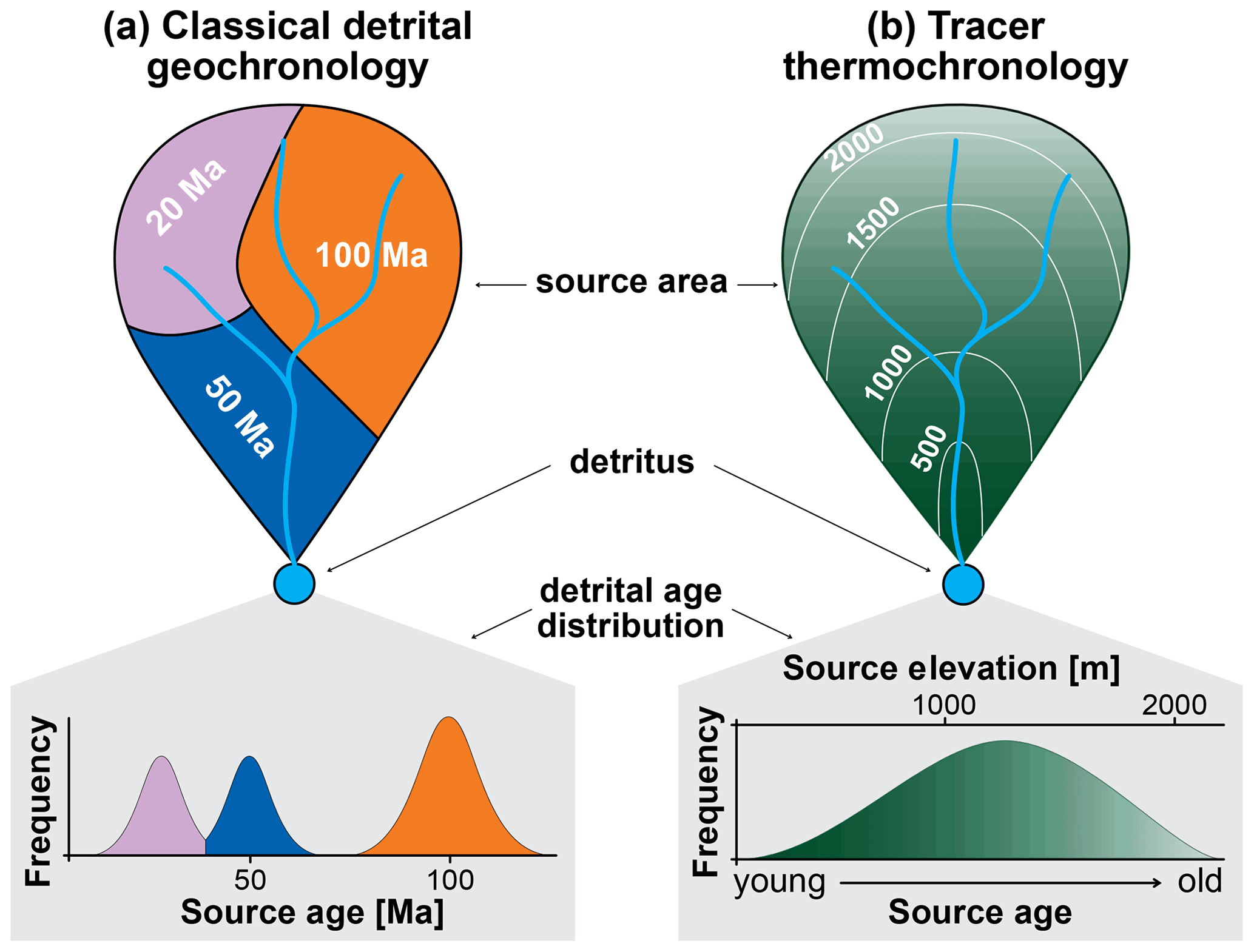
Figure 1 Sketch of the difference between classical detrital geochronology (a) and tracer thermochronology (b). (a) Discrete age components are found in the detritus and refer to different upstream geological units. (b) A continuous detrital age distribution informs the relative abundance of material sourced from different elevations based on a known age–elevation relationship.

In the following we summarize the conceptual model concerning this matter and the approaches that have been used to address it thus far. Let us consider a monolithologic catchment and a set of detrital grain ages measured at its outlet. The observed grain age distribution should match a predicted distribution that is forward-modeled by stacking the following layers of geologic information about the upstream area (Fig. 2).

• I.

  the catchment hypsometry, or the distribution of the catchment's cumulative area as a function of elevation, which is derived from the digital elevation model (DEM) of the study area and has a negligible uncertainty;

• II.

  the bedrock age–elevation data, which in the simplest case is a linear function based on a dataset of ages with associated uncertainty measured at known elevations;

• III.

  the mineral fertility, which informs the original abundance of the target mineral in the different elevation ranges and is mostly a function of lithologic variability and is a critical parameter that can lead to gross misinterpretations if ignored (Malusà et al., 2016);

• IV.

  information about how the sediment size distribution varies between the headwaters and the detritus, which is used to make sure that grains in the detritus are representative of erosion in the catchment (e.g., Vermeesch, 2007; Riebe et al., 2015; Lukens et al., 2020);

• V.

  the pattern of erosion across the catchment, which is the dependent variable of the system and can be any map of erosion probability used as a scenario to be tested against uniform erosion (or other reference scenarios).

Regardless of the scope of the application, tracer thermochronology ultimately aims to quantify the mismatch between observed and predicted distributions, where the predicted distributions vary depending on assumed models for catchment erosion, sediment dynamics, and tectonics.

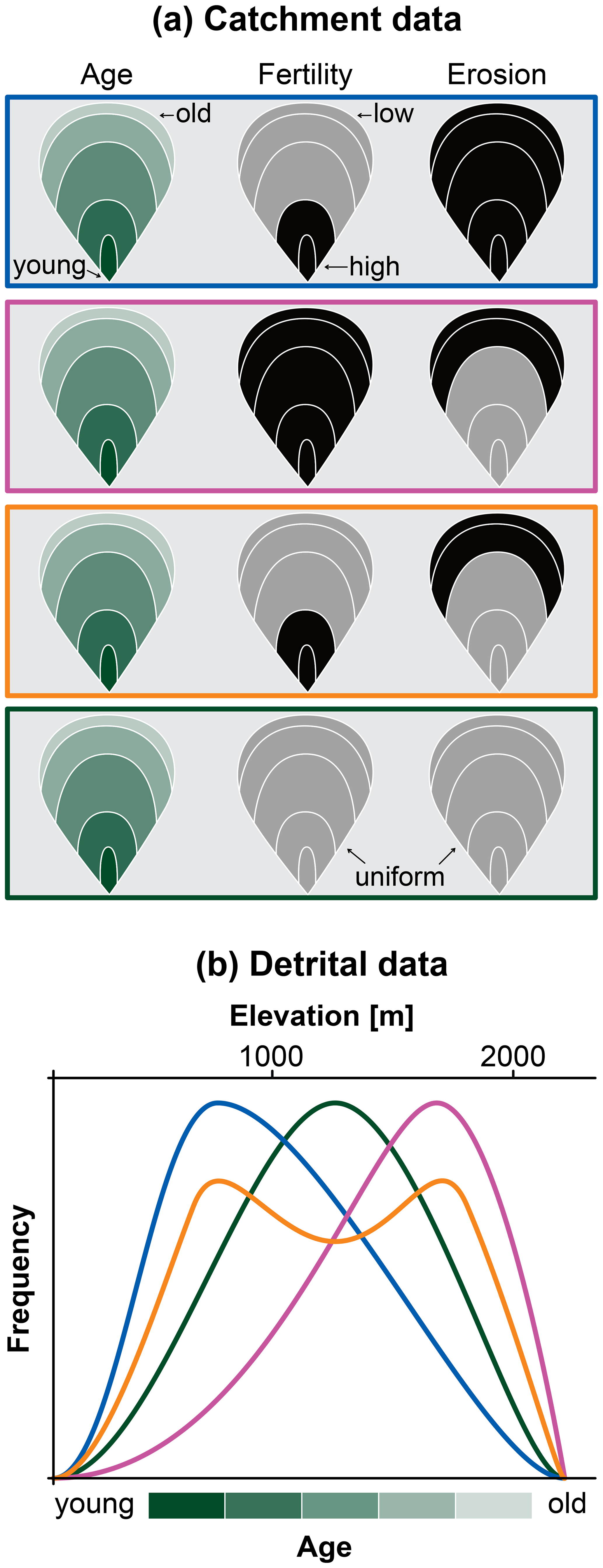
Figure 2 Qualitative sketch to illustrate the effect of mineral fertility and erosion on the detrital distribution. (a) The catchment of Fig. 1b with known bedrock age (shades of green) is subject to three scenarios of spatially varying fertility and erosion. The box outlines refer to the curves below. (b) Detrital distributions obtained from the different scenarios in (a). The green curve refers to spatially uniform erosion and fertility.

3 Comparing predicted and observed distributions

Predicted distributions should be constructed accounting for all of the above information and related uncertainties, such that the confidence of the fit to the observed distribution also accounts for them. Brewer et al. (2003), and later Ruhl and Hodges (2005), were the first to compare the distribution of detrital thermochronometers to that of age–elevation data. Although the scope of their work differed from more recent tracer thermochronology, the evaluation of the dissimilarity between predicted and observed distributions remains the main object of their studies. These authors constructed synoptic probability density functions (SPDFs) of the observed data by “stacking” the Gaussian distributions of all measured grain ages, each with their analytical error (this is equivalent to the SPDF_t in Table 1 of Vermeesch, 2007). In addition to the observed distribution, a predicted SPDF was also constructed with the same method, where the predicted grain ages are a random subsample of the hypsometric curve and are each given an arbitrary average uncertainty. Brewer et al. (2003) define the mismatch P_diff between observed and predicted SPDF with Eq. (1):

$$\begin{array}{}\text{(1)}& P_{\mathrm{diff}}={\displaystyle \frac{{\sum }_{t=\mathrm{0}}^{t=\mathrm{\infty }}\left|P_{\mathrm{1}}\left(t\right)-P_{\mathrm{2}}\left(t\right)\right|}{\mathrm{2}}}\times \mathrm{100},\end{array}$$

where (P₁ and P₂) are the probabilities of the two distributions calculated at each age step (t). P_diff relates to the area comprised between two SPDF in the age–frequency space. Brewer et al. (2003) calculate the 95 % confidence mismatch between observed and predicted SPDF through a Monte Carlo simulation.

Vermeesch (2007) has shown that, for the purpose of comparison, observed and predicted distributions are best expressed as a cumulative age distribution (CAD) rather than SPDF. A CAD is a step-function with the sorted mean ages on the x axis and the related quantiles on the y axis (Vermeesch, 2007). This method is preferred because it avoids the possible sources of bias introduced by (i) the choice of smoothing parameter in the kernel density estimations (KDEs), (ii) binning in histograms, and (iii) uncertainty-based weighting in the SPDF curves (Vermeesch, 2012). To evaluate the goodness of fit between observed and predicted CADs, Vermeesch (2007) uses the Kolmogorov–Smirnov (KS) statistic, which informs the maximum distance d_KS between two cumulative distribution functions as follows (Massey, 1951, and references therein):

$$\begin{array}{}\text{(2)}& d_{\mathrm{KS}}=\text{maximum}\left|{\text{CAD}}_{\mathrm{observed}}\left(t\right)-{\text{CAD}}_{\mathrm{predicted}}\left(t\right)\right|.\end{array}$$

Given an observed CAD with k observations (i.e., ages), d_KS is calculated for several n=k subsamples of the predicted CAD. The 95th percentile of all sorted d_KS (d_{KS_95}) is used as the least significant dissimilarity to reject the null hypothesis that the observations are drawn from the predicted CAD. In other words, an observed CAD that plots entirely within the range CAD_predicted±d_{KS_95} (Fig. 3) cannot be discerned from the predicted age population at the 95 % confidence level. As an alternative to this iterative method, the confidence region for a predicted CAD can be calculated with the analytical solution of the Dvoretzky–Kiefer–Wolfowitz (DKW) inequality as follows:

$$\begin{array}{}\text{(3)}& d_{\mathrm{KS}\mathrm{\_}\mathrm{95}}\approx \mathit{\epsilon }=\sqrt{{\displaystyle \frac{\ln \frac{\mathrm{2}}{\mathit{\alpha }}}{\mathrm{2}k}}},\end{array}$$

where the DKW distance ε approximates the d_{KS_95} well as a function of confidence level (1−α) and sample size k (Fig. 3) (Massart, 1990; Massey, 1951).

Figure 3 Example of metrics to compare two cumulative distributions drawn from different sample sizes. Here, an observed cumulative age distribution (CAD) for n=k (stepwise dashed orange line) is compared to a predicted CAD drawn for n≫k (solid black line). The Kolmogorov–Smirnov statistic d_KS equals the maximum absolute vertical distance between distributions in the observations–frequency space. The Kuiper statistic d_Kui equals the sum of both positive and negative maxima. For α=0.05 (i.e., 95 % confidence) and n=k, a Dvoretzky–Kiefer–Wolfowitz confidence region can be calculated (gray shading). In this example, observed and predicted distributions are drawn from two statistically different populations at the 95 % confidence level because the orange curve exceeds the gray region.

Riebe et al. (2015) further developed the bootstrapping approach described above to age distributions (in SPDF form). Instead of basing their analysis on the KS statistic, the 95 % confidence envelope of the prediction is iteratively estimated at each age step t_i. For each t_i, the distribution of 10 000 predicted age frequencies SPDF_predicted(t_i) is used to draw 2.5th and 97.5th percentiles at each age step. Because the age steps t_i relate to the elevation steps in the catchment through the bedrock thermochronometric data, those elevation steps exhibiting excess (>97.5th) or deficit (<2.5th) frequency are interpreted to produce sediment in excess or deficit with respect to the reference scenario of uniform erosion at the 95 % confidence level.

The approaches summarized above are well-suited to test observed detrital age distributions against the null hypothesis of spatially uniform erosion. However, even if the uniform erosion hypothesis is rejected, such a test does not yield further information about the spatial variability of sediment production. One way to gain additional information would be to test the observed distribution against predicted age distributions from erosion scenarios other than spatially uniform distributions, thereby quantifying the likelihood that the measured grain ages could be produced by the tested scenarios. This approach would help practitioners in deciding the sampling strategy, calculating the appropriate number of measurements and the resources to be allocated for them. In the next paragraphs we introduce the new ESD_thermotrace software, an open-source tool built on the cited previous work to consistently perform the following tasks: (i) determination of the confidence level allowed by the detrital sample size in rejecting the uniform erosion hypothesis, (ii) analysis of the statistical power of detecting the effect size caused by alternative erosion hypotheses as a function of the number of grains, and (iii) testing of observed detrital distributions against all input erosion hypotheses (both uniform and alternative scenarios) and calculation of the likelihood that the detrital sample may have been drawn from either of them. The software is introduced in the paragraphs below.

4 ESD_thermotrace: a tool to study the uncertainty of tracer thermochronology datasets

The software ESD_thermotrace (Madella et al., 2022) performs the steps briefly outlined below. For additional details, the reader is referred to the illustrative case study in Sect. 5 and the well-commented code itself (https://doi.org/10.5880/fidgeo.2021.003):

1. Bedrock age map interpolation.

   • Input. Bedrock age–elevation dataset and digital elevation model.

   • Output. Bedrock age map.

   • Method. Users can choose among 1D linear regression, 3D linear interpolation, 3D radial basis function. Alternatively, an externally produced age map can be imported.

2. Bedrock age uncertainty map interpolation.

   • Input. Bedrock age–elevation dataset with uncertainties (point data) and bedrock age map (grid data).

   • Output. Bedrock age uncertainty map.

   • Method. The uncertainty of the age map is estimated through bootstrapping. An externally produced uncertainty map is required if the age map was imported.

3. Catchment bedrock age, coordinates, mineral fertility, and erosion data extraction.

   • Input. Catchment outline, bedrock age and age uncertainty maps, mineral fertility map, and one or more erosion maps.

   • Output. A table of all the listed catchment properties necessary to predict detrital age distributions

   • Method. For each cell of the age map contained in the catchment outline, the local coordinates, age, fertility, and erosional weight(s) are extracted.

4. Detrital grain age distribution prediction for each erosion scenario.

   • Input. Table of catchment data.

   • Output. A predicted detrital age population for each erosion scenario and related cumulative age distribution.

   • Method. An amount of ages proportional to erosional weight and fertility is drawn from each cell for each scenario. The ages from all catchment cells collectively represent a predicted population from which cumulative age distributions are constructed.

5. Calculation of (i) the likelihood of rejecting the uniform erosion hypothesis with the observed sample size and (ii) the statistical power of discerning predicted erosion scenarios (i.e., alternative hypotheses) as a function of sample size.

   • Input. One or more sets of observed grain ages and uncertainties and predicted detrital populations and distributions.

   • Output. A graph displaying (i) the confidence of rejecting uniform erosion with the observed sample size and (ii) the statistical power curve of discerning the scenarios from uniform erosion by varying sample size.

   • Method. First, the d_{ks_95} for the available sample size k is calculated with Eq. (3). Following this, the likelihood that the observed n=k CAD is more dissimilar than the d_{ks_95} is calculated through bootstrapping. The same operation is also repeated for a range of sample sizes ($\mathrm{20}<k<\mathrm{130}$) in order to estimate the rise in confidence level caused by the increasing sample size (if the observed distribution and associated uncertainty remained identical despite the changing sample size). To calculate the statistical power of discerning the tested erosion hypotheses, the same approach is applied. In this case, however, the software draws a number of distributions from each erosion scenario instead of the observed grain ages.

6. Calculation of the plausibility of each erosion scenario (i.e., the likelihood that alternative hypotheses cannot be rejected with high confidence) given a set of observed detrital grain ages and uncertainties.

   • Input. One or more sets of observed grain ages and uncertainties and predicted detrital populations and distributions.

   • Output. Two plots to visualize how plausibly the observed grain ages have been drawn from the predictions.

   • Method. In the first plot, dissimilarities calculated between predictions and observations are sorted and their distribution is plotted in the form of a violin plot. Second, a two-dimensional multi-dimensional scaling (MDS) model is fitted to the dissimilarities among the predicted and observed distributions and plotted following Vermeesch (2013).

All of the above operations are embedded in an open-source Jupyter Notebook (https://jupyter.org/, last access: 22 March 2022), a software that allows for integrating text, Python code, and visualizations within the same document to make it as editable and transparent as possible. All plots are produced with Matplotlib (Hunter, 2007) and Seaborn (Waskom et al., 2020) Python libraries and are colored using the colorblind-friendly and perceptually uniform ScientificColourMaps6 (Crameri et al., 2020). In the following paragraph we show, for illustrative purposes only, how the program helps in analyzing an already published detrital apatite age dataset (Stock et al., 2006).

5 Application of ESD_thermotrace to the Inyo Creek case study

We apply ESD_thermotrace to the bedrock and detrital apatite (U-Th(-Sm)/He, hereafter AHe) age datasets of Stock et al. (2006). In that study, nine bedrock AHe ages from the Inyo Creek and adjacent Lone Pine Creek catchments (eastern Sierra Nevada, California, USA) are used to constrain the age–elevation relationship of the source area. The authors compared these bedrock data to the AHe age distribution of river sand samples from both catchment outlets. For the sake of simplicity, here we only consider the fine sand sample (k=52) from the Inyo Creek catchment. Based on their analysis, Stock et al. (2006) inferred no significant variability of sediment production (erosion) across all elevations within the catchment.

5.1 Data import and bedrock age interpolation

The first few steps of ESD_thermotrace allow for importing (i) the digital elevation model of the study area; (ii) the polygon of the catchment of interest; (iii) a table of bedrock age, age uncertainties, and elevation data; (iv) the (optional) erosion scenarios to be tested; and (v) an optional fertility map. Next, the surface bedrock ages are calculated with the preferred method (see above and the README file in Madella et al., 2022). The bedrock AHe ages of Stock et al. (2006), recalculated after Riebe et al. (2015), exhibit a ∼60 Myr age increase from ca. 2 to 4.5 km elevation range that is described well by an inverse variance-weighted linear regression (r²=0.93). The input data are plotted in Fig. 4a. In Fig. 4b, every cell is assigned an AHe age as a linear function of elevation (Fig. 5b) to map the bedrock cooling age on the topographic surface. The interpolation error is also mapped in Fig. 5a, and it displays the 1σ uncertainty of the prediction from the linear regression (Fig. 5b).

Figure 4 Input bedrock data from Stock et al. (2006). (a) Raster images of the study area's digital elevation model, resampled to the user-specific cell size, and (b) bedrock surface AHe age interpolated based on the linear regression of age–elevation data. In both plots, point data inform bedrock sample locations and related AHe ages. Polygons show the location of the Inyo Creek catchment.

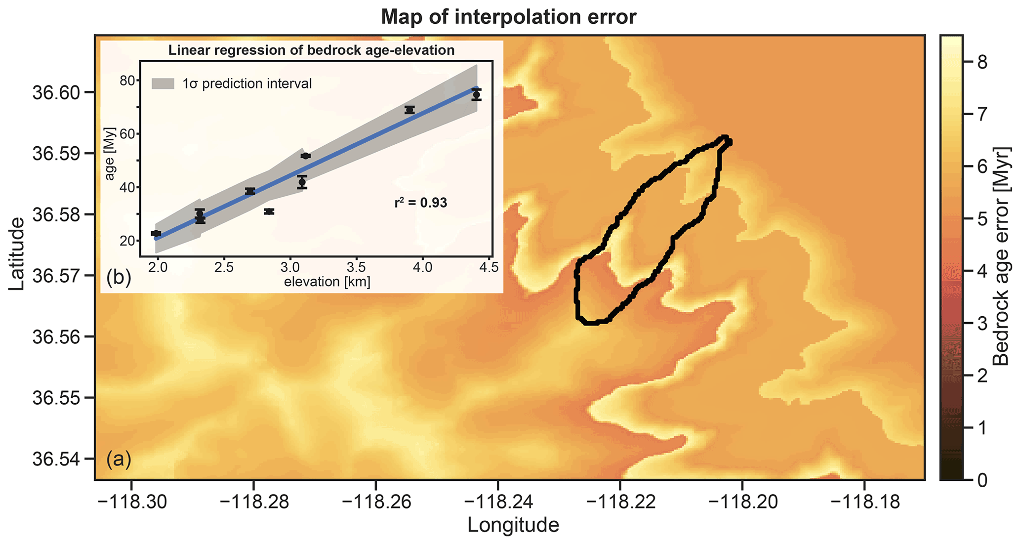
Figure 5 The raster image (a) displays the bedrock age interpolation error mapped to the topographic surface of the study area. The inset (b) shows the inverse variance-weighed linear regression employed as an age–elevation function, as well as the associated prediction interval with 1σ confidence level.

5.2 Extraction of catchment data

Next, ESD_thermotrace extracts the x, y, and z coordinates; the bedrock cooling age; and the related error for all the cells bound by the catchment outline. These data are written in a table, to which a column detailing erosional weights is added for each desired erosion scenario and for mineral fertility. In addition to the user-defined erosion maps, by default the software considers the uniform erosion scenario Euni (spatially constant erosional weight). Two further example scenarios can be toggled to test for an exponential increase of erosion with elevation or an exponential decrease of erosion with elevation (not considered here). We note that any other spatial variation in erosion can be defined by a user such that “erosion maps” for the catchment following stream power, slope dependency, glacial slide velocity, or other approaches from geomorphic transport laws can be input.

For this case study, bulk geochemistry and point-counting analyses of Hirt (2007) indicate that apatite fertility does not significantly vary within the three lithologies found in the Inyo Creek catchment (Lone Pine granodiorite, Paradise granodiorite, Whitney granodiorites). For illustrative purpose, we test uniform erosion against two opposite step functions of elevation: a scenario with F times higher erosion efficiency above the median catchment elevation and one with F times higher erosion below the median elevation. The factor F is equal to double the ratio between the most frequent and the least frequent elevation. For this calculation, the hypsometric histogram is constructed with a number of bins equal to the maximum difference in bedrock cooling ages, divided by the mean age uncertainty (rounded up to the next integer). Here, the Inyo Creek catchment is binned in seven elevation ranges, of which the most frequent is 5 times the least frequent one, resulting in F=10. In other words, we test for an increase in erosion twice as prominent as the hypsometric peak (10-fold), once below (“E<Z_med”) and once above (“E>Z_med”) the median catchment elevation.

5.3 Prediction of age populations and detrital age distributions

The erosional weights are used to forward model sediment production at each position in the catchment. To do so, an amount of grain ages proportional to the erosional weight and to the local mineral fertility are randomly chosen for each cell. These grain ages are randomly drawn from a normal distribution constructed using the local interpolated bedrock age and the related uncertainties. The randomly picked grain ages of all cells are stored in one suite of grain ages, which represents the predicted detrital grain age population of a well-mixed fluvial sediment at the catchment outlet. Such a detrital population is predicted for each erosion scenario, and related predicted CADs are constructed by sorting the age populations and plotted as a step function (Fig. 6b). For the sake of quick visual comparison, ESD_thermotrace plots a kernel density estimation with arbitrary smoothing (Fig. 6a). However, the dissimilarity among distributions will be evaluated exclusively based on the cumulative form in order to minimize bias (Vermeesch, 2007). In Fig. 6b, all predicted and observed cumulative age distributions are plotted. For a first-order impression of the uncertainty due to sample size, the 95 % confidence envelope of the reference scenario is also calculated with Eq. (3) and plotted in the background. Here, the user can specify for which reference scenario (“E_uni” as default) the confidence envelope should be plotted.

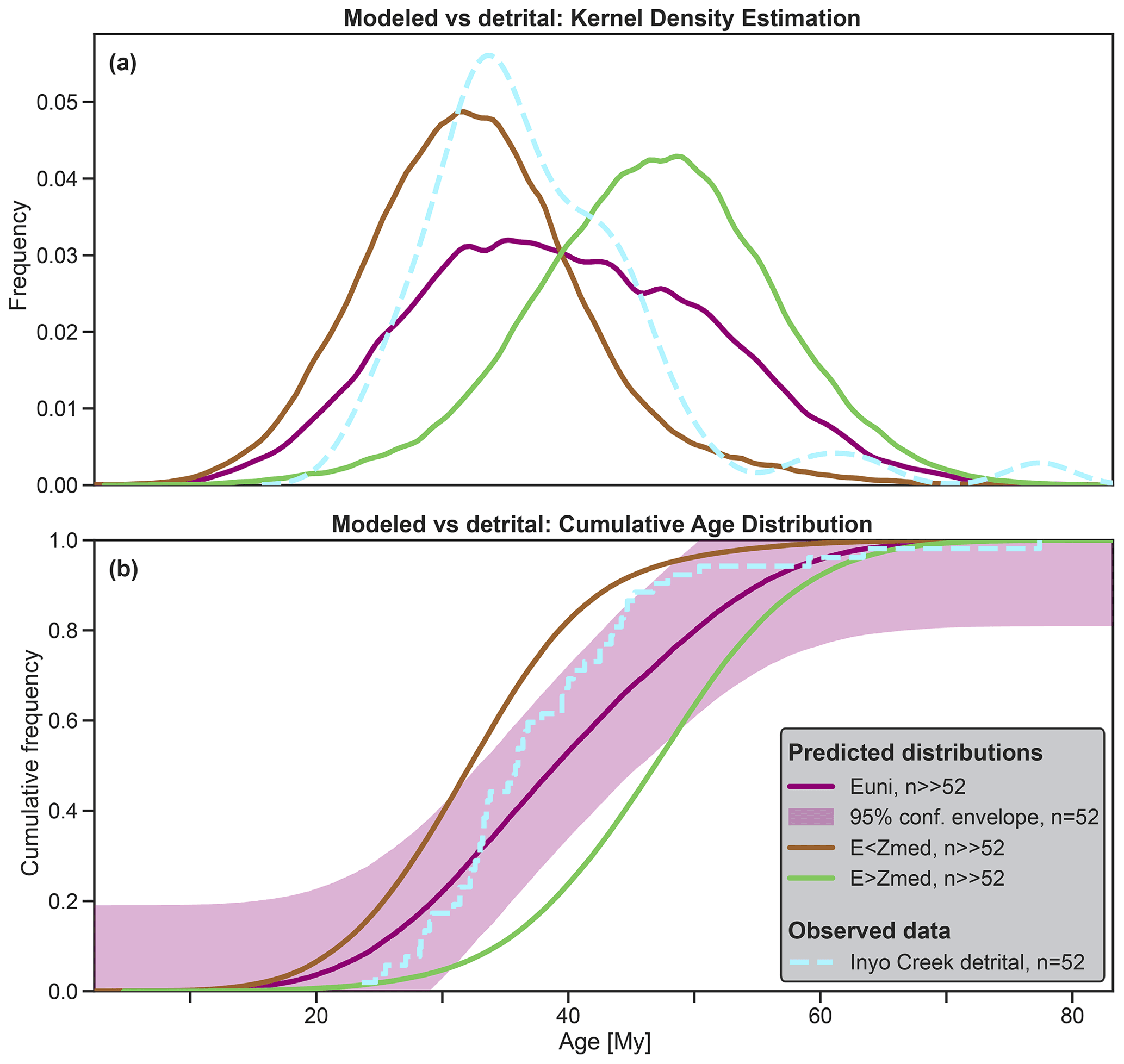
Figure 6 Kernel density estimation curves of all predicted detrital distributions and of the observed detrital sample (a). Cumulative form (b) of the same distributions, plus the 95 % confidence envelope (DKW-bounds) of “E_uni” for $n=k=\mathrm{52}$. E_uni indicates uniform erosion, E<Z_med indicates 10-fold erosion below median elevation, and E>Z_med indicates 10-fold erosion above median elevation.

5.4 Confidence level and statistical power as a function of sample size

After predicting the distributions, to answer the question of how many grain ages are necessary to discern a hypothetical erosion pattern from uniform erosion, the software analyzes the statistical confidence and the statistical power as a function of sample size. The confidence informs the likelihood of rejecting a null hypothesis H₀ (the uniform erosion scenario) based on the observations (the dated grains). The statistical power informs the likelihood that if an alternative hypothesis H₁ was true (one of the tested erosion scenarios), H₀ would be rejected based on a sample drawn from H₁. Here, the software calculates (i) the maximum confidence in rejecting the uniform erosion hypothesis allowed by the observed sample size and (ii) the statistical power of discerning the scenarios from uniform erosion as a function of sample size. Let us consider the observed CAD constructed with the sorted mean grain ages. The mean standard deviation of the observed grain ages is used to generate 10 000 Monte Carlo samples of this observed CAD, which account for age dispersion due to analytical error and/or reproducibility. Thus, the confidence in rejecting uniform erosion equals the fraction of sampled CADs that is more dissimilar to “E_uni” than the least significant dissimilarity (d_{KS_95}) allowed by the sample size k (see Eq. 3). The statistical confidence calculated in this manner can be read in the scatterplot of Fig. 7 (light blue circle), and it equals 55 % for the Stock et al. (2006) data. Figure 7 also shows that the 95 % level of significance could be achieved with more than 128 grain ages. Here, we clarify that the latter estimate assumes that the observed distribution would not change in shape while varying the sample size, and as such it can only be treated as an indicative number.

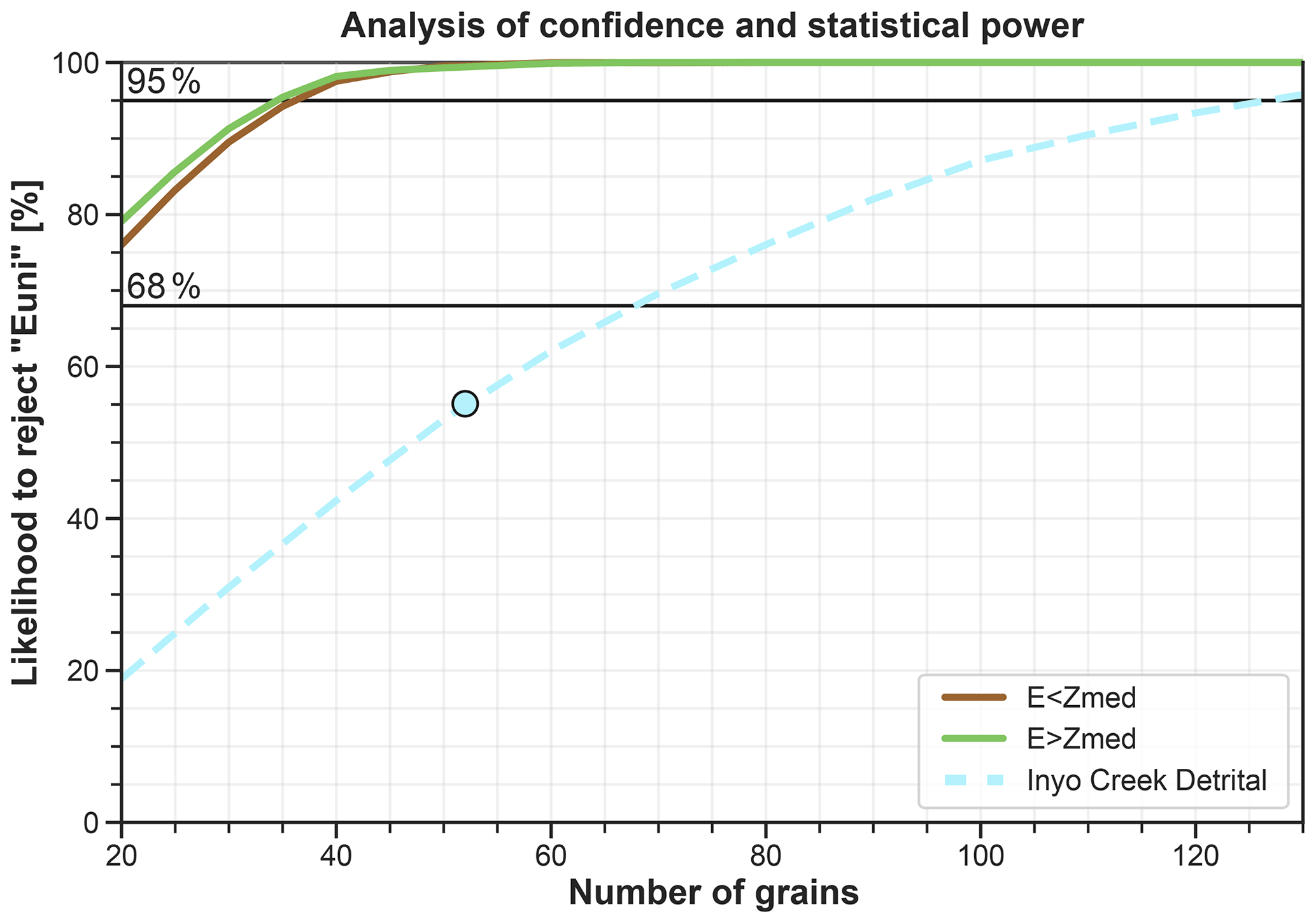
Figure 7 Confidence level at which the observed CAD (n=52) can be discerned from the uniform erosion prediction (cyan circle). The dashed cyan line shows how the allowed confidence level would vary if the same observed CAD relied on 20–130 grain ages. Statistical power of discerning the tested erosion scenarios from “E_uni” as function of sample size (solid lines). In this case study, the observed CAD of the Inyo Creek detrital sample allows rejecting the uniform erosion hypothesis with 55 % confidence at best. An analysis to detect the scenarios “E<Z_med” and “E>Z_med” would have a statistical power greater than 95 % in rejecting “E_uni” with more than 37 grain ages. E_uni indicates uniform erosion, E<Z_med indicates 10-fold erosion below median elevation, and E>Z_med indicates 10-fold erosion above median elevation.

If the confidence allowed by the actual sample size is lower than the previously chosen level of significance, the analysis of statistical power can help in identifying how likely the available number of grain ages would be to detect a known effect size (i.e., the dissimilarity caused by a known erosion scenario). This analysis of statistical power is based on the iterative comparison between the reference scenario and all other erosion scenario predictions. This is achieved through random subsampling of the predicted distributions for a range of possible sample sizes ($\mathrm{20}\le n\le \mathrm{130}$ in this case). For each n_i, the least significant dissimilarity d_{KS_95}(n_i)^* of the reference scenario is calculated for α=0.05 and n=n_i using Eq. (3). In the observations–cumulative frequency space (Fig. 6b), d_{KS_95}(n_i)^* represents the vertical distance that any n=n_i distribution needs to exceed to be discerned from a n=n_i subsample of the reference scenario with 95 % confidence (purple shading in Fig. 6b). Next, 1000 d_{KS_95}(n_i) are calculated between n=n_i subsamples of each erosion scenario and the reference scenario. The probability of d_{KS_95}(n_i) exceeding d_{KS_95}(n_i)^* for each n_i can be read from the curves in Fig. 7. For the Inyo Creek case study (Stock et al., 2006), both tested erosion scenarios (“E<Z_med”, “E>Z_med”) yield predicted CADs that are very dissimilar from uniform erosion. Consequently, the statistical power to discern these alternative erosion hypotheses would exceed 95 % even with only 40 grains.

Figure 7 shows the use of ESD_thermotrace as a tool to explore the feasibility of a tracer thermochronology study. Based on their research question, users can apply a few possible erosion maps and test the likelihood with which the respective detrital distributions could be discerned from uniform erosion through detrital tracer thermochronology as a function of sample size. Such analysis of feasibility is not only beneficial in terms of better quantifying uncertainties, but it can also assist investigators in defining the budget for measurements at an early stage of proposal writing. Alternatively, in cases where the number of datable grains is limited by material properties, budget, or other logistical reasons, Fig. 7 informs the maximum confidence level of the results.

5.5 Evaluating the plausibility of test scenarios

The final steps of ESD_thermotrace assist users in finding the erosion scenario that is most likely to generate a predicted CAD that resembles the observed CAD. For each erosion scenario, d_KS and d_Kui (Fig. 3) are calculated between 10 000 n=k subsamples of the respective predicted CAD and the observed CAD. The distribution of these d_KS and d_Kui values is shown in the form of a split violin plot in Fig. 8a, and it is to be compared to the range of values shown by the violin in Fig. 8b. The latter shows the distribution of d_KS and d_Kui calculated between random subsamples of the observed CAD that account for the mean analytical error and the observed CAD itself (constructed only with the mean ages). In other words, Fig. 8b displays how the dispersion of a predicted CAD (accounting for analytical error and sample size) is distributed. The “plausibility” of each scenario is plotted beneath each violin and it equals the probability that the values plotted in Fig. 8a fall within the one-sided lower 95th percentile of those shown in Fig. 8b. For the sake of clarity, we note that the term “plausibility” used here is equivalent to the false negative rate (β) in statistical jargon. Accordingly, there is 51.6 % probability that the observed CAD could be drawn from the uniform erosion scenario, and 13.7 % and 0.0 % probability that scenarios “E<Z_med” and “E>Z_med” generate predicted CADs that fall within the spread of the observed CAD, respectively.

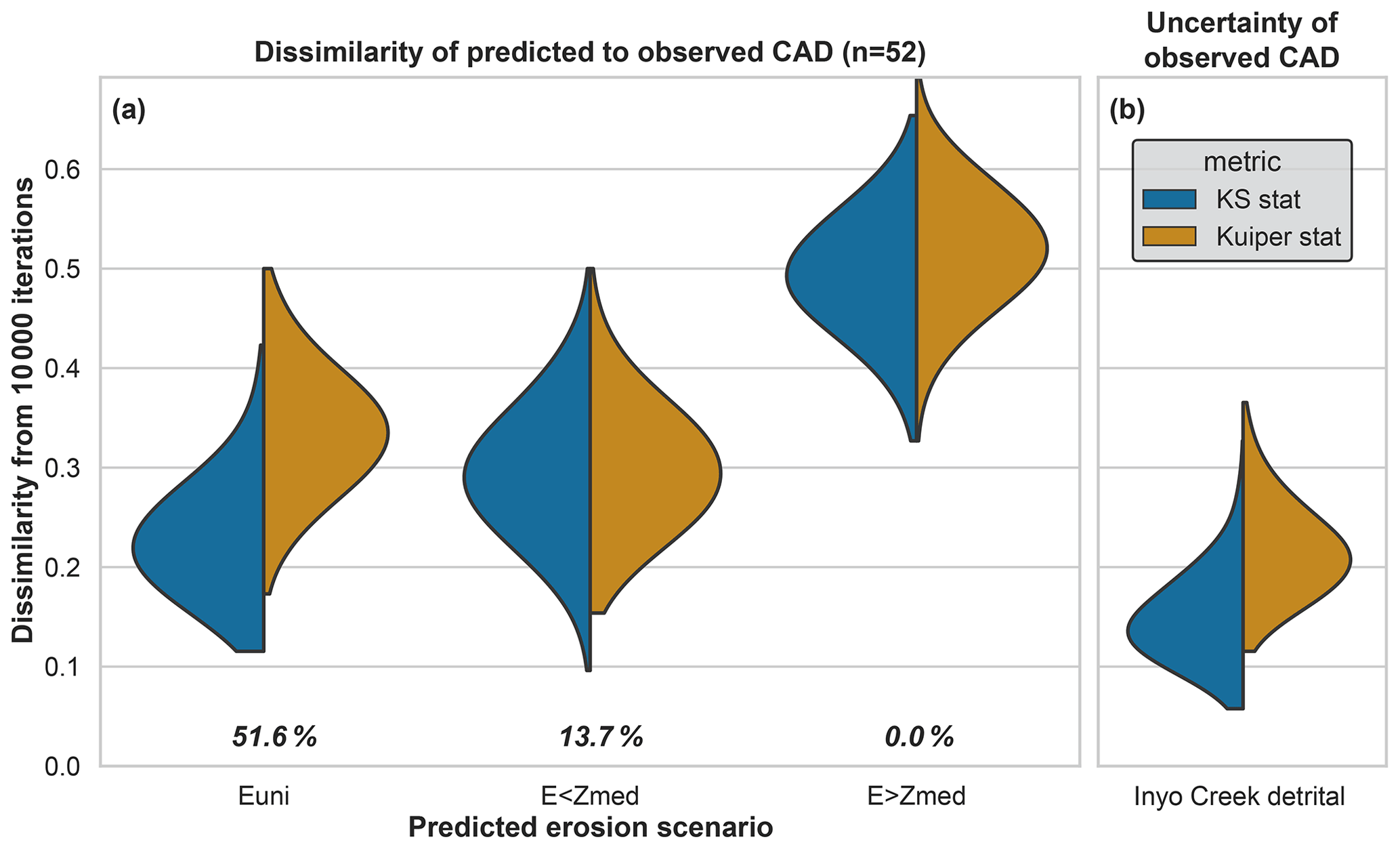
Figure 8 Violin plot showing the KS (and Kuiper) statistics between the predicted CAD of each erosion scenario and observed CAD, calculated for 1000 $n=k=\mathrm{52}$ subsamples (a). KS (and Kuiper) statistics between the observed CAD and 10 000 random $n=k=\mathrm{52}$ distributions, drawn from the same detrital age population but including uncertainty (b). Every violin is split in two halves with equal area, each representing the probability distribution function of 10 000 KS (or Kuiper) statistics. The widest point of each semi-violin informs the most frequent KS (or Kuiper) statistic. The closer this value is to zero, the more similar the scenario is to the observed detrital age distribution. The most unlikely scenario is “E>Z_med”. Both other scenarios are plausible because their dissimilarity to the observed CAD largely overlaps the range of dissimilarity due to analytical error of the detrital ages.

Lastly, as suggested by Vermeesch (2013), the ESD_thermotrace program applies a two-component multi-dimensional scaling model (MDS) to all predicted and observed distributions. This algorithm fits a two-dimensional coordinate system to the measured dissimilarities d_KS among all considered distributions (both predicted and observed). In a well-fitted MDS model, distances among points in the modeled 2D space are a good approximation of the actual dissimilarities among the input elements (Fig. 9a). To reach a satisfactory fit, modeled dissimilarities are plotted against input dissimilarities (Fig. 9b) and the sum of all distances to the 1:1 line is minimized (a procedure commonly referred to as stress minimization). The MDS plot renders an immediate visualization of the dissimilarity among distributions, where more similar distributions plot closer to each other. Moreover, with the addition of the 68 % and 95 % confidence ellipses, the degree of overlap among distributions is also easily visually assessed (Fig. 9a).

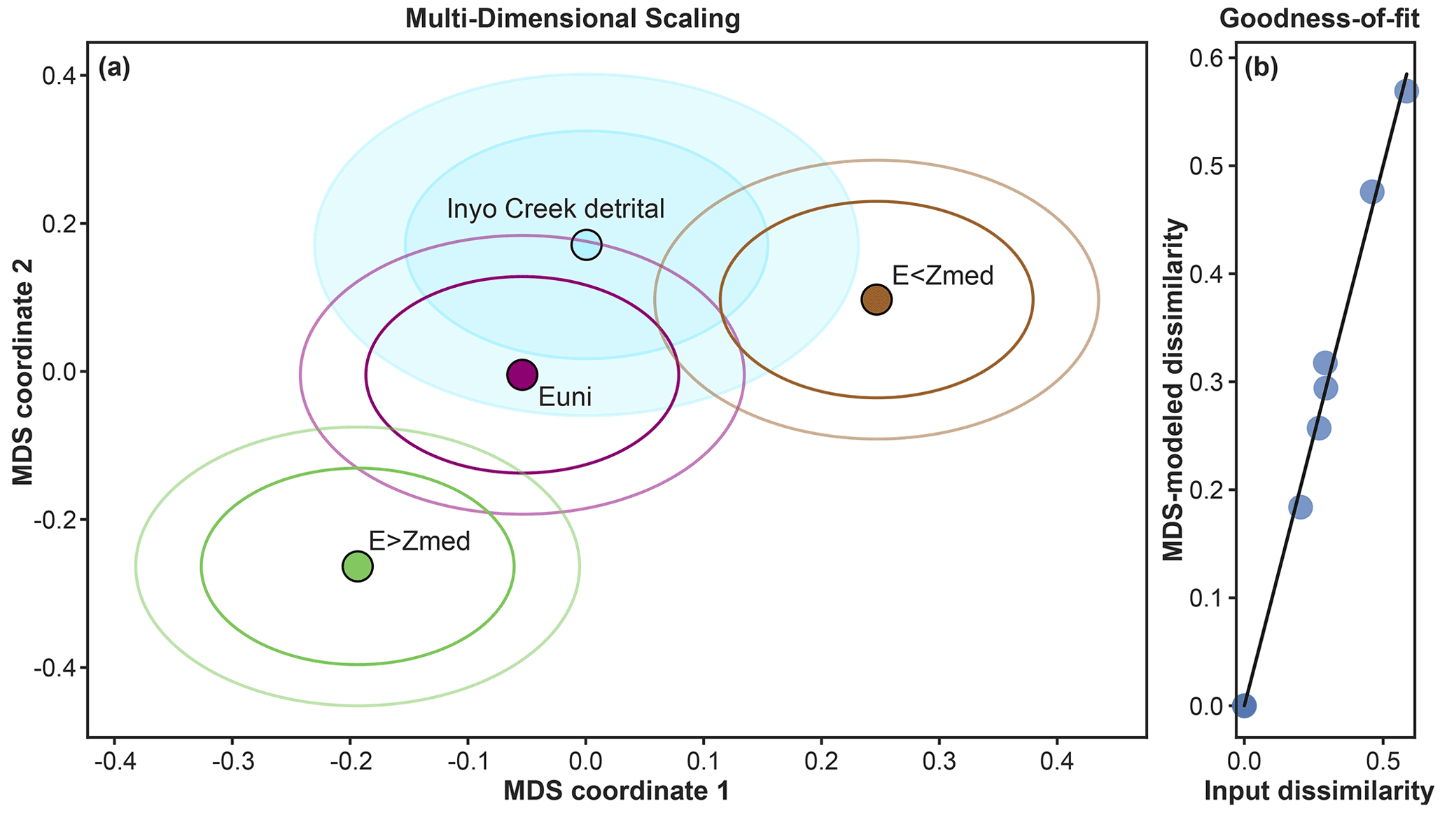
Figure 9 Multi-dimensional scaling (MDS) plot. The two-component MDS model fits a coordinate system to the measured dissimilarities (i.e., KS statistics) among all distributions. If the MDS model has a good fit, distances calculated in the new 2D space (a) are a good approximation of the input dissimilarities among the elements. The goodness of fit is shown in (b), where modeled dissimilarities are plotted against input dissimilarities. For each distribution in (a), 68 % and 95 % confidence ellipses are also plotted.

The application of the ESD_thermotrace software to the Inyo Creek data of Stock et al. (2006) shows the following characteristics.

• A sample size of 52 grain ages allows a maximum confidence level of ∼55 % in rejecting the uniform erosion hypothesis “E_uni” (cyan circle in Fig. 7). If the observed CAD had been drawn from ∼130 grain ages, this confidence level would exceed 95 % (dashed cyan curve in Fig. 7).

• A total of 52 grain ages would suffice to detect the effect size caused by “E<Z_med” and “E>Z_med” (green and brown curves in Fig. 7). However, the observed detrital sample is extremely unlikely to have been drawn from either of these scenarios.

• Among the tested scenarios, the uniform erosion hypothesis “E_uni” is the least dissimilar (51.6 % likelihood) (Figs. 8 and 9).

Here, while we have shown the functioning of ESD_thermotrace using the Inyo Creek data from Stock et al. (2006), we refrain from proposing a revised interpretation of the catchment's erosion dynamics. We do note that, in addition to the data from Stock et al. (2006), Riebe et al. (2015) have accounted for ¹⁰Be-derived denudation rates and 73 additional AHe ages from coarse sand-sized sediment. These authors have shown that erosion in the Inyo Creek catchment is best explained by an exponential increase of sediment production with elevation. Thereby, they demonstrate that understanding the pattern of erosion in this catchment requires taking multiple sediment sizes into account (Riebe et al., 2015; Lukens et al., 2020; Sklar et al., 2020; see also discussion below).

6 How many grains do we need for tracer thermochronology?

The analysis with ESD_thermotrace shows that the appropriate sample size for a tracer thermochronology study cannot be determined a priori without knowing (i) the case-specific scientific question (i.e., the spatial pattern of erosion to be tested), (ii) the source area hypsometry, (iii) the desired minimum confidence level, and (iv) the surface bedrock ages and uncertainties. On this note, if possible, it is advisable to explore the feasibility of a study with the already available bedrock ages before sampling. In absence of available published ages, bedrock samples are best processed first to avoid wasting resources on potentially inconclusive analyses of detrital grains. To better illustrate the importance of the initial knowledge of the catchment's geology, we conducted a set of simulations with the same inputs as the Inyo Creek case study (Stock et al., 2006). In these simulations we vary the location (in terms of elevation range) of maximal erosion and observe the impact on the statistical power in detecting the imposed pattern. Both a broad and a narrow Gaussian curve of erosion (1σ=500 and 100 m, respectively) are applied to the catchment's range of elevations, shifting the position of the peak in 100 m steps at each simulation. We test two sets of Gaussian functions of elevation computed in such a way that the prominence of peak erosion equals 2 times and 5 times the prominence of the catchment's hypsometric peak, respectively. Therefore, because the most frequent elevation range is ca. 5 times the least frequent bin (Fig. 10c, f), the “2×” and “5×” curves define an erosion efficiency where peak sediment production is 10 times and 25 times higher than the minimum in the catchment, respectively. Results from this parameter study, example erosional functions, and the hypsometric histogram are illustrated in Fig. 10.

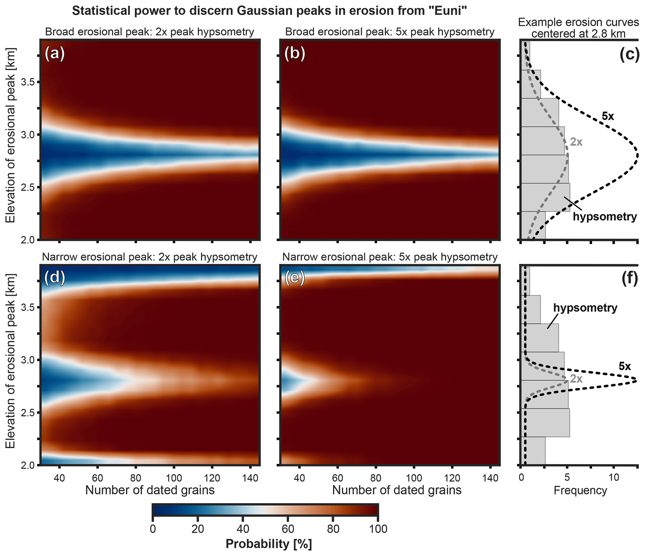
Figure 10 Analysis of statistical power in discerning between the uniform erosion scenario “E_uni” and scenarios with a broad (a, b) or narrow (d, e) Gaussian peak of erosion as a function of sample size and elevation of the Gaussian peak. The color scale informs the statistical power as a function of the number of grains (x axis) and the elevation at which the Gaussian peak is centered (y axis). The catchment hypsometry (c, f) and age–elevation relationship used here are the same as the Inyo Creek data (Stock et al., 2006). (a) Gaussian erosional function with 1σ=500 m and 2 times the peak prominence of the hypsometric histogram. (b) Gaussian erosional function with 1σ=500 m and 5 times the peak prominence of the hypsometric histogram. (d) Gaussian erosional function with 1σ=100 m and 2 times the peak prominence of the hypsometric histogram. (e) Gaussian erosional function with 1σ=100 m and 5 times the peak prominence of the hypsometric histogram. (c, f) Example erosional functions for peaks centered at 2800 m elevation. The reader is referred to Sect. 6 for more details.

Figure 10 shows how the statistical power in detecting these Gaussian peak scenarios is affected by (i) the elevation of the erosional peak, (ii) its amplitude, (iii) its width, and (iv) the detrital sample size. An increase in sample size and/or an increase in amplitude of the erosional peak always correspond to higher statistical power. The elevation of the erosional peak affects the statistical power depending on the position of the erosional peak relative to the peak of hypsometry (Fig. 10). In the case of a broad Gaussian function of erosion (1σ=500 m), minima (blue areas) are observed where the erosional peak is located at elevations straddling 2800 m (Fig. 10a, b). These minima in statistical power at ∼2800 m coincide with the broad frequency peak of catchment elevations (Fig. 10c). In this elevation range, the diffused increase in erosion efficiency does accentuate the peak of the hypsometric curve, but it results in a limited effect size (i.e., a small d_KS dissimilarity to “E_uni”). With this configuration, all erosion scenarios peaking within ca. 2700–2900 m produce detrital distributions whose effect size is detected in only <60 % of the simulations, regardless of sample size and peak amplitude. This implies that certain combinations of erosional pattern and distribution of bedrock age are poorly suited to be investigated by means of tracer thermochronology.

In the case of a narrow Gaussian function of erosion (1σ=100 m) (Fig. 10d, e, f), minima of statistical power are additionally found at peak elevations higher than 3600 m and lower than 2200 m (Fig. 10d, e). These occur because peak erosion is applied to a narrow elevation range that is not frequent enough to produce a statistically relevant number of grains. However, in the case of narrow erosional peaks, an increase in sample size substantially increases the statistical power to detect erosion scenarios, even if it is centered at the critical elevation of ca. 2700–2900 m described above (Fig. 10d, e). This parameter study demonstrates the importance of analyzing the catchment hypsometry and testing erosion scenarios even before collecting data in order to make an informed choice on the appropriate sample sizes and to identify possible scenarios that are unlikely to be detected with high confidence through detrital tracer thermochronology.

7 Other sources of uncertainty

The approach presented here for predicting and interpreting grain age distributions enables quantifying the confidence level in rejecting the uniform erosion hypothesis and the statistical power in discerning a prescribed erosion scenario from uniform erosion through detrital tracer thermochronology. Confidence level and statistical power are computed as a function of the sample size, the catchment properties, and input erosion scenario. Nevertheless, even if the plausibility of a scenario is inferred to be high, our software by design does not suggest a unique solution and interpretations are also subject to additional sources of uncertainty. These include (1) complex bedrock age–elevation relationships (Malusà and Fitzgerald, 2020) and (2) spatial variability of sediment size resulting from transport distances (e.g., Lukens et al., 2020; Malusà and Garzanti, 2019), geomorphic processes (e.g., Riebe et al., 2015; van Dongen et al., 2019), lithological differences (von Eynatten et al., 2012), or vegetation effects on weathering and erosion (Starke et al., 2020). Both factors should be considered, as discussed below.

In some cases, elevation alone cannot explain the entire variance of bedrock thermochronometric ages. For example, spatial variability of bedrock ages may reflect the proximity to tectonic structures or sub-catchment thermal events (e.g., magmatism, spatial changes in thermal gradients in proximity of major faults). In such cases, an improved sampling of the spatial distribution of bedrock ages is needed and may require more complex interpolation functions (e.g., Glotzbach et al., 2013). To accommodate these complexities, ESD_thermotrace allows for 1D and 3D linear interpolation and radial basis function interpolation. In all of these cases, the interpolated age uncertainty is calculated through bootstrapping. In addition, users can opt to import an independently interpolated surface bedrock map from a thermokinematic model for example (e.g., Whipp and Ehlers, 2019). For additional information on bedrock thermochronometric age mapping the reader is referred to the README file included with the software (Madella et al., 2022). Regardless of which method is used, users should be aware that different interpolation methods may yield different predicted distributions, depending on the quality of the bedrock data. Accordingly, resulting interpolated surfaces should be carefully evaluated, and a preference should be motivated by field observations and/or independent constraints. Here, the map of interpolated age uncertainty can also inform the locations where additional bedrock sampling would help reduce the uncertainty. Lastly, we note that an increase in age uncertainty always determines the decrease in the statistical power of the analysis.

Other possible sources of bias concern the grain size of the analyzed samples. Several issues may modify the original fingerprint of river sand (Malusà and Garzanti, 2019), such as downstream grain abrasion and fracturing, hydraulic sorting, and weathering on the hillslope associated with a grain (Attal and Lavé, 2009). For example, grains sourced the farthest from the sampling spot may be underrepresented in the analyzed grain size fraction (Lukens et al., 2020), as has also been shown for the Inyo Creek catchment (Sklar et al., 2020). Furthermore, in addition to the mineral fertility inherent to the exposed bedrock, the grain size distribution of the material found on the hillslopes (i.e., the material ready for transport) should be taken into account. Depending on the lithology (von Eynatten et al., 2012; Roda-Boluda et al., 2018) and on the locally dominant denudation process (van Dongen et al., 2019), different hillslopes of the same catchment may produce substantially different sediment size distributions (e.g., Riebe et al., 2015; Attal et al., 2015). Consequently, the mixed detrital sample may exhibit a bias in the relative abundance of the different age components. Both of these issues can be mitigated through analysis of multiple grain size fractions (Lukens et al., 2020), multiple measures of hillslope sediment size distributions, composite analyses of trunk stream and tributary stream sediment samples, and analyses of thermochronometers from different minerals.

8 Conclusion

This study reviewed previous approaches used to compare predicted and observed detrital grain age distributions in the framework of tracer thermochronology. We have built upon these to develop a new tool (ESD_thermotrace) to investigate the upstream pattern of catchment erosion and the confidence level in uniquely inferring this as a function of sample size and study-site-specific variables. To demonstrate the utility of this approach, we presented an analysis of previously published data from the Inyo Creek catchment in California. The example highlighted the utility of measuring a large number of grains, and how multiple erosion scenarios are plausible for this catchment with the considered number of grains. The degree of statistical confidence permitted by this case study has also been quantified. We showed how the use of ESD_thermotrace can increase the statistical rigor of tracer thermochronology studies and how it can also assist investigators in budgeting analytical costs of a future project. In cases where the number of datable grains is limited, the confidence level of the results can be quantified, and the statistical power of the analysis can also be estimated.