sandbox – creating and analysing synthetic sediment sections with R

Past environmental information is typically inferred from proxy data contained in accretionary sediments. The validity of proxy data and analysis workflows are usually assumed implicitly, with systematic tests and uncertainty estimates restricted to modern analogue studies or reduced-complexity case studies. However, a more generic and consistent approach to exploring the validity and variability of proxy functions would be to translate a sediment section into a model scenario: a “virtual twin”. Here, we introduce a conceptual framework and numerical tool set that allows the definition and analysis of synthetic sediment sections. The R package sandbox describes arbitrary stratigraphically consistent deposits by depth-dependent rules and grain-specific parameters, allowing full scalability and flexibility. Virtual samples can be taken, resulting in discrete grain mixtures with defined parameters. These samples can be virtually prepared and analysed, for example to test hypotheses. We illustrate the concept of sandbox, explain how a sediment section can be mapped into the model and explore geochronological research questions related to the effects of sample geometry and grain-size-specific age inheritance. We summarise further application scenarios of the model framework, relevant for but not restricted to the broader geochronological community.

1 Introduction

Information about the evolution of earth-surface dynamics beyond the time span of instrumental records is predominantly gathered from sediment deposits, serving as host material of proxy data. Proxies are based on the presupposition that a specific sediment property is representative of an unknown environmental variable or can be unequivocally converted into such. The validity of proxies is usually an assumption based on conceptual relationships, modern analogue data, or physical principles. Further implicit assumptions arise from practical and methodological constraints, such as minimal post-depositional alteration, representative sampling, appropriate sample preparation and measurement, and robust estimation of uncertainty ranges. All these preconditions are typically assumed or at least considered to be of generic validity, but their impact on the interpretations is rarely tested.

Numerical modelling of the earth surface processes has reached an advanced level (Willgoose et al., 1991; Schoorl et al., 2000; Tucker et al., 2001; Lowry et al., 2013; Hobley et al., 2017). Yet, the commonly utilised landscape evolution models almost exclusively focus on specific parts of the terrestrial sediment cascade, such as weathering, erosion, and material transport processes, or at least have model-specific strengths and weaknesses in representing elements of this process phalanx. However, the formation of sediment deposits as proxy carriers is rarely considered. Most often, sediment is simply flushed out of the terminal node or pixel of the modelled area, or deposition is reduced to the pure formation of geometric bodies (e.g. Lowry et al., 2013). Despite its importance, the host material of our environmental information is significantly understudied from a numerical perspective.

Describing a sediment deposit by a model would include a geometric description of the entire body (width, length, depth) as well as a thematic description of its constituents (e.g. voids, grains and their geometrical, mineralogical, or chemical composition) by a vast number of parameters. As an example, describing a 10 m deep and 1 m wide and long column of loess would require describing as many as 10¹⁴ single grains, and each by a series of parameters. Depending on the research question, one might reduce the geometric dimension of the deposit and thus the number of individual constituents to describe. Likewise, it is possible to limit the number of parameters used to define each constituent. However, the general challenge remains. An alternative to this geometric and parametric reductionist approach is a model not at the scale of its discrete constituents but one with model-wide rules that describe the properties of potential constituents at any given location within the sedimentary deposit.

Here, we introduce the R package sandbox, a novel framework to create virtual sediment deposits. We explain the concept and structure of sandbox along with a step-by-step description of how to map a “real-world” loess section into a model. We illustrate different potential applications using simple examples, acknowledging that more realistic representations are possible with additional parameterisation efforts. While we focus on geochronometric data, various other applications can be pursued. The Supplement contains an extensive tutorial to the package, elaborated examples on how to implement more realistic deposition effects, and all code used to create the figures of this article.

2 Philosophy and structure of sandbox

sandbox is a free and open framework to build and analyse virtual sediment sections in R (R Development Core Team, 2021). The package (Dietze and Kreutzer, 2021) is available at the Comprehensive R Archive Network (CRAN). The current developer version is available on GitHub (https://github.com/coffeemuggler/sandbox/, last access: 19 May 2022). The term framework implies that sandbox is not tailored to a specific task but instead provides methods to use the tool in different scenarios. Specifically, sandbox does not impose any default physical rules to mimic sedimentation processes. Nevertheless, such process-based rules can be implemented if desired (see the Supplement for examples). Users can reduce or expand the default range of parameters applied to describe the constituents of a sediment section.

sandbox is essentially a one-dimensional model. It describes the geometry of a sedimentary deposit only by its depth while assuming infinite width and length. Boundary conditions are treated as irrelevant apart from the distance to surface.

sandbox has a parametric (termed rule-based from here on) and probabilistic design. Sediment properties are defined by depth-dependent rules, containing the definitions of grain properties as probability density function parameters.

sandbox allows the user not only to build synthetic sediment sections but also to sample them, prepare the samples, measure them, and work with the synthetic results as with real-world measurement data. The function make_Sample() generates a finite number of sediment particles based on the rule-controlled parameters together with information on the sampling depth and sample container geometry. This step is the transition from rule-based to the discrete data realm.

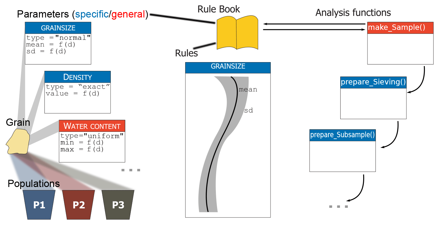
Figure 1 Concept of the model sandbox. Grains are the atomic elements of the model. They are drawn from populations and assigned parameters, which in turn are controlled by rules. Both rules and parameters are stored in rule books that act as coherent reference objects. Preparation functions are used to virtually process samples that are generated based on rule books.

Understanding sandbox (Fig. 1) requires some key terms used in the modelling environment:

• Population. A population is the most basic, coherent element of the entire model. A population is a set of sediment grains with common characteristics. All grains from one population share the same (range of) properties of certain parameters, such as grain size, depositional age, or mineralogic composition.

• Grain. Grains are the atomic elements of the model. They are always sampled from populations and described by a set of parameters. Each population has a defined probability of occurrence, which is defined as a parameter.

• Parameter. Parameters are used to describe populations and, hence, sediment grains drawn from these populations. They can be seen as the “thematic” definition of a virtual sediment deposit. There are two major groups of parameters: general and specific. General parameters are depth-dependent sediment descriptions regardless of the population the grains are sampled from. Examples of general parameters are water content and external dose rate (ionising radiation per time unit). Specific parameters describe sediment grains with respect to the population to which a grain belongs. Hence, for each population, there is another parameter definition. Examples are grain size, element or mineral constituents, and specific density.

• Rule. Rules describe how parameters change with depth. Rules can be regarded as the “spatial” definition of a sediment deposit. They are defined as interpolation functions based on parameter–depth relationships. The default interpolation function is a spline.

• Rule book. A rule book is the combination of parameters (“thematic” definition) and rules (“spatial” definition) to one coherent reference book. A rule book ultimately comprises the definition of the entire virtual sediment section and generates individual samples. There is an empty rule book available by default. A user can modify a rule book’s content at any time.

• Analysis function. Once a rule book defines a virtual sediment deposit, it can be “exploited” using the pre-selection of available functions, for example, by generating sets of samples with make_Sample(). These samples can then be subject to additional analysis functions of the package, such as prepare_Sieving() and prepare_Subsample(). All these prepare-functions use information stored in each grain.

3 Materials and methods

3.1 Available functions

To start from scratch, it is necessary to create a new empty rule book, which can then be expanded by adding rules and parameters. A new rule book can be created by the function get_RuleBook(), using the default keyword book = "empty".

		book <- get_RuleBook(book = "empty")

This will generate a list object with all principal elements required to define a virtual sediment section: a book name ($book); a true age definition ($age); and the definition of population likelihoods ($population), grain sizes ($grainsize), packing density ($packing), and specific grain density ($density).

True age means that there is an initial age for each grain depending on its depth. With depths and ages defined at discrete intervals and interpolated by a spline function, sandbox uses a very simplistic representation of the sediment accumulation process by default. It does not account for hiatuses or autocorrelated incremental sedimentation pulses followed by pauses (Blaauw and Christen, 2011). However, such dedicated relationships can be implemented if required (see the Supplement for examples).

Grain sizes are defined on a ϕ scale throughout ($\mathit{\varphi }=-{\log }_{\mathrm{2}}\left(\frac{D}{D_{\mathrm{0}}}\right)$, with D the diameter in µm and D₀ the reference diameter 1000 µm) to account for the non-normal distribution of these data (Krumbein, 1937). Packing density describes the ratio between compound sample volume and the volume of solid particles in that sample. For regular spheres in a 3D space, the close-packing density cannot exceed 0.74 (Hales, 1992). For natural soil material, the packing density is usually around 0.3 to 0.6 (Blume et al., 2010). The packing density becomes relevant for sandbox when taking virtual samples by volume or further volume-based processing steps. The specific grain density (2.65 g cm⁻³ for quartz) is needed to define grain masses.

The function add_Population() allows other grain populations to be added to a rule book, which by default only has one. Populations can be added at any time, and all specific rules of the rule book will be updated for the respective number of additional populations. The function requires specifying the rule book to be updated and providing the number of populations to add.

Using add_Rule() allows expansion of the range of applications and addition of, for example, information about the chemical or mineralogical composition of a sediment section. The new rule will automatically add the corresponding new parameter. The function requires specifying the rule book to be changed (book), a name (name) for the new rule and corresponding parameter, whether it is a specific or general rule (group), and how the resulting parameter is allowed to vary (type). Possible variation types are type = "exact" (no variation), type = "normal" (variability according to a normal distribution defined by additional rules of mean and standard deviation), type = "uniform" (variability according to a uniform distribution defined by minimum and maximum values), and type = "gamma" (variability following a Gamma distribution defined by its shape and scale parameters as well as an offset constant). Depending on the type of variability, the function will add the required parameters (value, mean, sd, min, max, shape, scale, offset) to the rule book. To add, for example, a rule that defines a uniformly varying pH value for all populations, the following code is needed:

		book3 <- add_Rule(book = book,
		         name = "pH",
		         group = "general",
		         type = "uniform")

The function set_Rule() allows the actual rules of the rule book to be defined. An empty rule book just contains the templates of required rules (five in total). These templates need to be filled with proper definitions. This is the main purpose of set_Rule(). Depending on how a rule defines the parameter variability, one needs to provide different information along with their respective depth intervals to establish the right interpolation function. To define the rule for grain depositional ages, one needs to define a list that contains the depth intervals for the corresponding true age information and assign this to the rule book. To assign grain density rules, allowing for variability around a mean with a given standard deviation, one needs to create a nested list, one for each population, containing the means and standard deviations at the corresponding depth intervals. The below example will first define the rules as a 1 m depth interval, with a linear age increase of 1 ka m⁻¹. Then, the density for the population (P1) is defined as 2.5 g cm⁻³ on average, but with a depth-dependent standard deviation. Finally, the grain packing density is set to 0.5 without scatter throughout the sediment section.

## describe rule definitions
depth <- list(c(0, 1, 2, 3))
age <- list(c(0, 1000, 2000, 3000))
density <- list(P1 = list(
 mean = c(2.5, 2.5, 2.5, 2.5),
 sd = c(0.0, 0.1, 0.2, 0.0)))
packing <- list(
 P1 = list(mean = rep(0.5, 4),
 sd = rep(0, 4)))

## assign age rule
book <- set_Rule(
 book = book,
 parameter = "age",
 value = age,
 depth = depth)

## assign density rule
book <- set_Rule(
 book = book,
 parameter = "density",
 value = density,
 depth = depth)

## assign packing rule
book <- set_Rule(
 book = book,
 parameter = "packing",
 value = packing,
 depth = depth)

make_Sample() is a special function used to turn the essential information of a rule book into a discrete set of n grains. For this, the function requires the arguments book (the rule book used to define the sediment section), depth (defining the centroid depth where the sample is created), and geometry (defining the geometrical shape of the sample container). Currently, two types of sample containers are implemented: "cuboid" and "cylinder". Depending on which of the two container shapes is used, further input is needed regarding height, width, length, and radius. The function output is a data.frame object with all grains, each described by the parameters contained in the rule book. The following code snippet creates a 1 cm³ large sample cube:

## assign packing rule
sample_1 <- make_Sample(
 book = book,
 depth = 1,
 geometry = "cuboid",
 height = 0.01,
 width = 0.01,
 length = 0.01)

With prepare_Sieving(), one can simulate the physical sieving of a sample. The function requires the arguments sample (the sample object to be processed) and interval (sieve interval in ϕ units). Based on this information, it will remove all grains from the sample object that do not fall into the sieve intervals and return the updated data set.

Splitting a bulk sample into a set of subsamples is performed by the function prepare_Subsample(). This can be done by splitting a sample into a defined number of equally large subsamples (specified by the argument number), by creating subsets of a defined volume (specified by the argument volume), or by creating subsamples defined by sample weight (specified using the argument weight). In the latter two cases, the remainder of the bulk sample that does not allow the last subsample to be filled will be rejected. The volume option accounts for the packing density, and the weight option accounts for the specific density of the sample grains.

A special kind of subsampling is performed by the function prepare_Aliquot(). Aliquots are defined in luminescence analysis as sample subsets that compose a monolayer of sediment, fixed onto small metal discs, supplied to the measurement device. The function mimics this typical workflow step and requires the specification of the aliquot disc size containing the grain monolayer and a packing density of the grains on that disc, usually 0.65. Note that this value differs from the original packing density value used to define the rule book.

Finally, the package contains a convenience function convert_units(). This function can be used to convert grain-size units between the metric and the ϕ scale. Note that the package also contains a further function add_Parameter(), which is a helper function used by set_Rule(), and not for direct usage.

3.2 The loess deposit Gleina

We use a 17 m thick real-world loess deposit from a former brickyard in the Saxonian Loess Region, eastern Germany (Meszner et al., 2011, 2013; Meszner, 2015). For this site, we can access a detailed granulometric data set (Meszner et al., 2021) along with a geochronological framework (Zech et al., 2017), both suitable in the context of this study.

The grain-size distribution of all 42 samples of the loess section were measured with a Horiba LA950 laser particle sizer, providing 98 grain-size classes. About 0.5 to 1.5 mg air-dried and homogenised material were treated with 10 % HCl for 24 h and subsequently treated with 40 % H₂O₂ for 72 h. Each sample was measured for 5 s with ultrasonic excitation for 10 s in the device to disaggregate particles mechanically. We used the Mie scattering theory with a refraction index of 1.55 and an absorption index of 1.33. The median distribution of 10 consecutive measurements per sample has been exported for further analyses.

3.3 EMMAgeo as auxiliary tool

To convert the quasi-continuous grain-size distributions into discrete populations, i.e. parametric descriptions (mean and standard deviation) of grain-size rules for sandbox, we unmixed the data set using the R package EMMAgeo v0.9.6 (Dietze and Dietze, 2016, 2019). This package allows end-member modelling analysis (EMMA) of grain-size data sets; it describes grain-size distributions as a linear combination of end-member loadings and scores. Loadings are the fundamental, genetically interpretable grain-size distributions inherent to all grains. They can be interpreted in terms of discrete sediment sources, transport pathways, and/or transport processes. Scores depict the contribution of each loading to each sample and can be considered as a description of the relevance of a transport process for a given sample. In the context of this study, loadings refer to the grain-size distribution of particular populations (parameter definition), and scores refer to the depth-dependent likelihood of a population to be sampled (rule definition). Here, we used deterministic EMMA with three end-members (q=3) and no transformation (l=0). The resulting loadings were approximated with log-normal distribution functions (i.e. normal distribution functions in the ϕ space) to get the best-fit values of mean and standard deviation for each of the three populations.

3.4 Mapping a deposit into sandbox

All analytical data of the Gleina loess section (Meszner et al., 2011), including the reanalysed grain-size data and end-member scores, were linearly interpolated to equal intervals of 25 cm, starting at 0.5 m depth and ending at 10.75 m depth (see the Supplement for details on the data set). We used the fine-grain luminescence ages (Zech et al., 2017) to build an interpolated age–depth relationship as true age–depth information, despite potential ambiguities, just for the sake of simplicity and to serve as an example.

We created a new empty rule book (gleina) and added two more grain populations to the default one, to accommodate the three end-members. Their relative contributions (depth-dependent scores, EM_scores) were used as population probabilities and added to the rule book. The parametric approximations of the end-member grain-size distributions (EM_gsd) were added as grain-size rules. We set the population-specific packing densities to 0.7 for the coarse-grained end-member, 0.6 for the medium, and 0.5 for the fine end-members, each with a standard deviation of 0.01. Grain-specific densities were set to 2.65 ± 0.01 g cm⁻³ for all populations, imposing predominantly quartz minerals. The following code snippet is a one-to-one version of this descriptive text.

## load the measurement data
X <- read.table(
 file = "gleina_interpolated.txt",
 header = TRUE)

## convert cm to m, get number of records
X$depth_int <- X$depth_int / 100
n <- nrow(X)

## create empty rule book
gleina <- get_RuleBook(book = "empty")

## add two further populations
gleina <- add_Population(book = gleina,
populations = 2)

## assign rule definitions to lists
depth <- list(X$depth_int)
age <- list(X$age_int)
EM_scores <- list(
 list(X$EM_1),
 list(X$EM_2),
 list(X$EM_3))
EM_gsd <- list(
 list(mean = rep(6.38, n),
      sd = rep(0.9, n)),
 list(mean = rep(4.69, n),
      sd = rep(0.5, n)),
 list(mean = rep(4.29, n),
      sd = rep(0.5, n)))
EM_packing <- list(
 list(mean = rep(0.7, n),
      sd = rep(0.01, n)),
 list(mean = rep(0.6, n),
      sd = rep(0.01, n)),
 list(mean = rep(0.5, n),
 sd = rep(0.01, n)))
EM_density <- list(
 list(mean = rep(2.65, n),
      sd = rep(0.01, n)),
 list(mean = rep(2.65, n),
      sd = rep(0.01, n)),
 list(mean = rep(2.65, n),
      sd = rep(0.01, n)))

## add rule definitions
gleina <- set_Rule(
 book = gleina,
 parameter = "age",
 value = age,
 depth = depth)
gleina <- set_Rule(
 book = gleina,
 parameter = "population",
 value = EM_scores,
 depth = depth)
gleina <- set_Rule(
 book = gleina,
 parameter = "grainsize",
 value = EM_gsd,
 depth = depth)
gleina <- set_Rule(
 book = gleina,
 parameter = "packing",
 value = EM_packing,
 depth = depth)
gleina <- set_Rule(
 book = gleina,
 parameter = "density",
 value = EM_density,
 depth = depth)

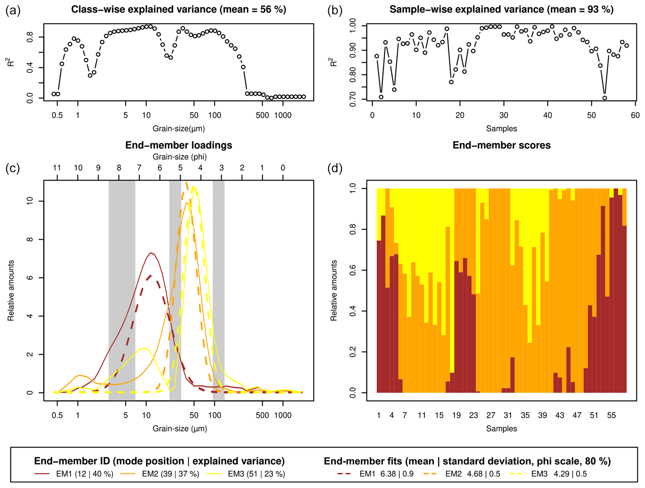
Figure 2 End-member modelling results of the measured grain-size data of the Gleina section. Dashed lines in the loadings plot show fitted log-normal distribution curves according to the parameters in the bottom legend panel. Grey shaded areas in the loadings panel depict grain-size intervals used for sieving to enrich individual end-members. Sample IDs in the scores plot denote samples from top to bottom.

3.5 Application examples and parameterisation

To illustrate the basic functionality and potential applicability of sandbox, we investigate three simple research questions and two more elaborated examples. The main goal of these tests is not to create the most realistic representations of depositional processes and resulting sediment sections, but rather to illustrate how parameters are defined, samples are examined, and the model's flexibility can be utilised. See the Supplement for the actual code implementation along with additional examples on more realistic physical process representation. The questions are as follows:

1. How does the sample container geometry impact the age scatter? Container geometry means that we have inspected the differences between cylindric and cuboid sample containers, all with the same volume. We simulated cylinders with 10 mm diameter; cubes of 10 mm width and height and 0.8 mm length; and cuboids of 20, 40, and 80 mm width and 5, 2.5, and 1.25 mm height, respectively. While the real-world applicability of such container geometries is limited, the test stresses the influence of sampling depth intervals, including minimal values. It can also be interpreted as mimicking the manual extraction of a thin sediment layer. Cuboid container lengths were set to 0.8 mm throughout. Note that we can work directly with the sampled material without any further preparation steps. Thus, small sample volumes are sufficient. The virtual sampling depth for the test was set to 5 m, using the depth-interpolated true ages of the sampled grains as a direct proxy for age scatter.

2. What is the effect of sample container size on age uncertainty? Here we test different cylinder diameters for different profile depths of the Gleina loess section. We have sampled the virtual Gleina section at 1 m intervals, using containers with diameters ranging from 0.5 to 50 cm, keeping the volume constant at 0.5 cm³. Again, 0.5 and 50 cm wide containers are far from reality. However, they define a safe lower and upper limit of possible cases and manually collected samples. This second question differs from the first one by also accounting for the deposition rate as the expected depth-dependent age span in a sample.

3. What kind of luminescence age bias can be expected due to preparation using standard grain-size intervals if the three components building the loess section have different bleaching probabilities? The rationale for this question is that sediment deposits are typically composed of material from different sources, contributed by different processes. Depending on the transport mechanism (for example low-energy but far-distance aeolian transport versus high-energy night-time hill wash), the exposure of grains to daylight may differ and so may the resetting likelihood of their luminescence signal. Poorly bleached grains with an inherited luminescence signal will appear older than their actual last transport event. At the same time, different transport mechanisms or energies will contribute grains of different size, hence linking age inheritance with grain size. Over time, the relative importance of transport processes with such different bleaching potential may change and so may the convoluted age inheritance effect at different depths of a sediment section. For this test, we have added a new specific rule (inherited), which defines an inherited age in years for each population. For the coarse-grained population (end-member 3), we assumed a poor bleaching likelihood and thus a uniformly distributed random age inheritance within the arbitrarily chosen range of 0 years to 5000 years. For the two other populations, we imposed uniform random inheritance ages between 0 and 200 years. We collected samples every 0.5 m using a 5 cm cylinder, sieved the sampled material for the typical coarse-grain (90–200 µm) and fine-grain (4–11 µm) fraction (e.g. Kreutzer et al., 2012a) and calculated the mean age composed of the true deposition age and the inheritance from each grain. In addition, we have prepared three additional data sets, this time adjusting the limits of the virtual sieve to isolate each of the three end-members as well as possible (see Fig. 2 for intervals), in order to inspect the age differences inherent to the three different components that constitute the sediment section.

4. How can depth-dependent packing densities be realised? While the above examples mainly aimed at abstract and simplified sediment section properties, one might also want to implement more physically or sedimentologically meaningful rules. Exemplarily, we show how a variable, depth-dependent packing density can be implemented. This example may be used when modelling successive sediment compaction with depth due to increasing overburden. For this, we use a simple porosity model (Sheldon and Retallack, 2001) to modify the packing density as a function of depth.

5. How can heteromorphism due to distinct mineral grain specific densities be implemented? This example simulates the transport of equally heavy grains of different size, a case that can be expected for sediment of inhomogeneous composition. To parameterise this example, we change one of the three populations of the existing rule book, i.e. the smallest grain population corresponding to end-member 1, allowing for it to be either composed of quartz (specific density of 2650 kg m⁻³) or zircon (specific density 4600 kg m⁻³). The diameter of the zircon grains is then calculated to result in an equal weight as the larger quartz grains. To make the effects visible, we additionally change the grain-size standard deviation of end-member 1 from 0.9 to 0.1. We note that this still is a simplified approach not fully in agreement with drag force constraints. Nevertheless, it serves the illustration of the generic approach.

4 Results

4.1 End-member modelling analysis

Deterministic EMMA (Fig. 2) resulted in an overall R² of 0.74 (sample-wise R²=0.93, class-wise R²=0.56). The three end-members were unimodal with ϕ modes at 6.38, 4.68, and 4.29 (12, 39, and 51 µm). Secondary artificial modes occurred below the main modes of the other end-members, as commonly encountered in EMMA (Dietze and Dietze, 2019). Hence, normal functions were only fitted to the primary modes. The best fits were reached for ϕ 6.38 ± 0.9, 4.68 ± 0.5, and 4.29 ± 0.5.

4.2 Effect of sample container geometry and size on age scatter

The sample container shape directly reflects the single-grain age distribution of the sampled material (Fig. 3). Cylinders produce a sinusoidal distribution shape of ages with a standard deviation of 3.7 years, while cubic containers produce a flat distribution with a standard deviation of 4.2 years. Note that the absolute scatter is an arbitrary number with no real-world equivalent. It merely depends on the deposition rate and container size (see below). Along that line, as the cuboids become more elongated in the horizontal direction by factors 2, 4, and 8, the standard deviations of the flat age distributions decrease to 2.1, 1.1, and 0.5 years, respectively. This purely geometric effect is also witnessed by the constant average age for all types of sampling containers.

Figure 3 Effect of sample container geometry on scatter of sampled grain ages. X axes all scaled to the same range.

Sample container size has a variable effect on the age scatter (Fig. 4), also depending on the deposition rate of the investigated sediment section. In general, larger sample container sizes systematically increase the age scatter inherent to the sampled grains, following a linear relationship. However, the sampling depth modulates the overall scatter, which determines the sediment deposition rate here. For the deposition ranges of the virtual Gleina section, we found age scatter as high as 4624 years (using a 50 cm wide sampling depth interval) in the basal section with a deposition rate of 0.033 m ka⁻¹. More realistically, 5 cm wide sampling containers still yielded an age scatter of 481 years. In the central parts of the section with deposition rates as high as 3.9 m ka⁻¹, that error reduced to 4 and 43 years for container diameters of 5 and 50 cm, respectively.

Figure 4 Effect of cylindric sample container size. Warmer colours indicate a higher age scatter.

4.3 OSL age bias due to prepared grain-size ranges

The impact of age inheritance can range from marginal to significant, depending on the analysed grain size fraction. Note that here we can ignore analytical scatter in age and thus error bars in Fig. 5 because we implicitly know the true ages of the sampled grains and focus completely on the systematic effects. Analysing the typically utilised coarse-grain fraction (90–200 µm, Fig. 5a) can introduce a systematic mean difference between apparent and true age of up to 2500 years (up to 10 %). That offset is controlled by the relative contribution of the coarse-grained end-member to a sample. The result is a stratigraphically inconsistent age–depth relationship with four age inversions. When using the typically encountered size interval of the fine-grain fraction (4–11 µm, Fig. 5b) to estimate average grain ages, the age offset is minimal, about 118 years on average. There are no age inversions visible in this size fraction. However, the age offset still correlates with the contribution of end-member 1, from which a few grains still leak into the sieve interval.

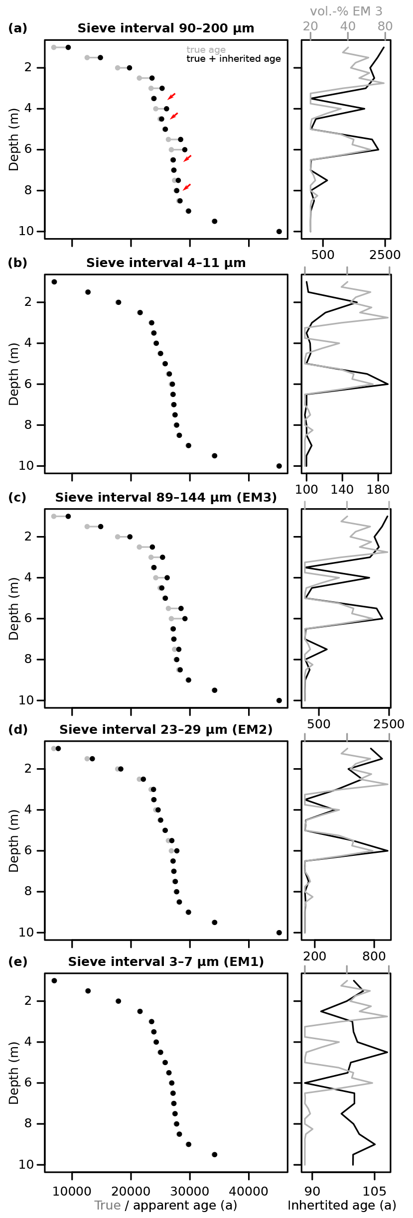
Figure 5 Age inheritance effects due to different sieve intervals of the modelled Gleina section. (a) Typical coarse-grain sieve intervals. (b) Typical fine-grain sieve intervals. (c–e) Optimised sieve intervals to isolate the three inherent grain-size end-members as well as possible. See Fig. 2 for interval definitions. The left plot panels show average true depositional ages (grey dots) and apparent measurement ages (black dots), composed of true and inherited ages per grain. Right plot panels show age inheritance (black lines) and contribution of end-member 1 (grey lines) as a function of depth. Red arrows mark age inversions.

When targeting grain-size intervals that specifically aim to isolate the three end-members inherent to the grain-size distribution of all samples, the coarse-grain end-member (Fig. 5c) mimics the offset and stratigraphic inversion patterns of the coarse-grain samples. The intermediate end-member (Fig. 5d) shows similar trends to the coarse one but with less severe effects (800 years maximum offset). Finally, the fine-grain end-member (Fig. 5e) shows an average age offset of 100 years (corresponding to the imposed range of 0–200 years) without any relationship to the contribution of the coarse-grained end-member.

4.4 Depth-dependent packing density behaviour

The simulation of a depth-dependent packing density relationship first required the function that relates these two metrics to be defined, following the porosity model by Sheldon and Retallack (2001).
rho_depth <- rho_qz - rho_qz * rho_0 *
exp(-k * X$depth_int)
Here rho_qz is the specific quartz grain density (2650 kg m⁻³); rho_0 is the initial relative porosity at zero depth, for loessic material typically around 0.6 (Blume et al., 2010); and k is an empirical material dependent compaction rate coefficient, here arbitrarily set to 10⁻¹. In a second step, this depth-dependent packing density can simply be added as a rule for all three populations of the existing rule book, for example with a constant scatter of 10 kg m⁻³ (rho_scatter <- rep(10, length(rho_depth))). The resulting depth-dependent packing density (Fig. 6a) follows the expected exponential trend.

gleina_packing <- set_Rule(
 book = gleina,
 parameter = "packing",
 value = list(
  list(mean = rho_depth,
       sd = rho_scatter),
  list(mean = rho_depth,
       sd = rho_scatter),
  list(mean = rho_depth,
       sd = rho_scatter)),
 depth = depth)

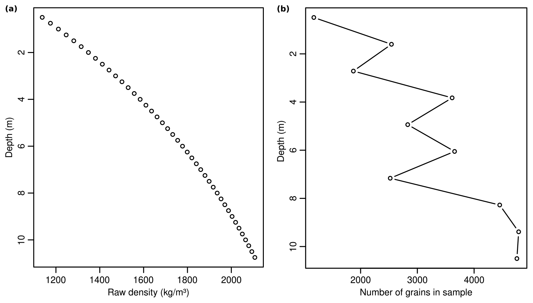
Figure 6 Depth-dependent sediment packing density evolution and resulting effects of generated samples. (a) Exponential relationship of depth and packing density following the model by Sheldon and Retallack (2001) with a decisively high compaction rate of 10⁻¹. (b) Resulting increasing number of grains per equally large sample containers (2 m sampling interval), showing some scatter due to the also depth-dependent contribution of populations of different size.

Sampling the modified rule book at 2 m sampling intervals with small containers (0.05 mm cuboid edge size) resembles the effect that denser packing yields in general more grains with increasing depth. However, the trend is superimposed by the also depth-dependent contribution of the three end-members, each with a different grain size.

4.5 Heteromorphism of grains with distinct specific density

To implement an equal contribution of grains from two populations of equal grain mass but correspondingly different mineral density, and hence diameter, we first determined the mass of a 1 mm large quartz grain and used this mass to solve for the diameter of an equally heavy zircon grain to retrieve the diameter conversion factor (i.e, 83.20754 %).

m_sand <- 2650 * (4/3 * pi * 0.00053)
d_zirc = 2 * (m_sand / (4/3 * pi * 4600))(1/3)
f_conversion <- d_zirc * 100 / 0.001

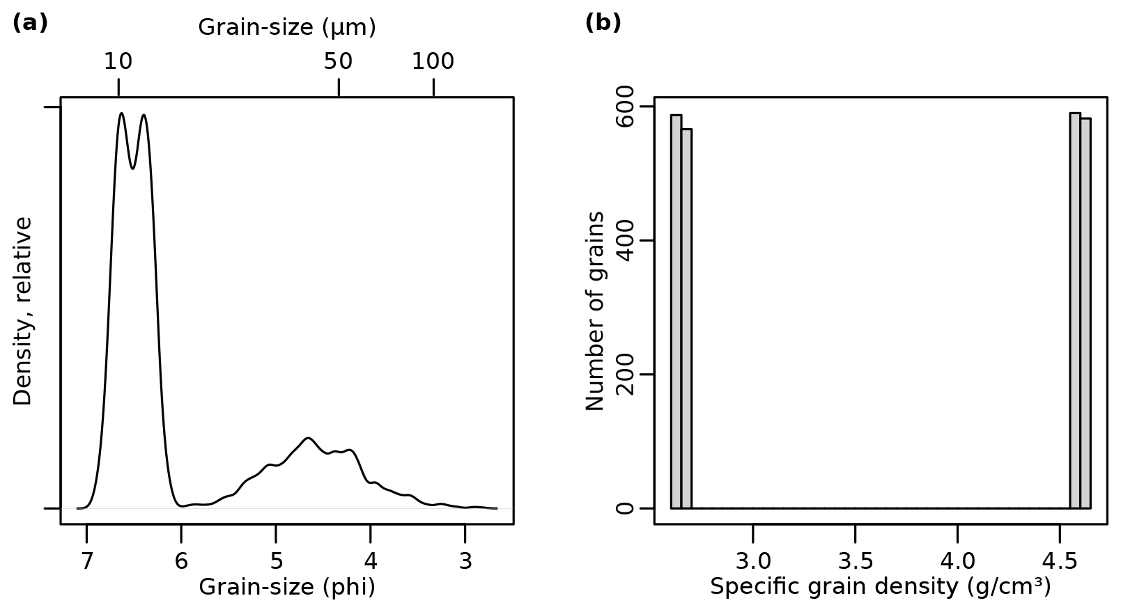
Figure 7 Properties of a virtual sample created at a depth of 11 m from a rule book with both quartz and zircon grains (see the Supplement for details). (a) Grain-size distribution, dominated by narrow distributions (0.1 ϕ standard deviation) of a quartz end-member 1 (6.38 ϕ) and an additional zircon population (6.65 ϕ) as well as suppressed minor contributions of coarser quartz end-members. (b) Histogram of the specific grain densities of all grains, showing a roughly equal occurrence of the two dominant populations of quartz (2650 kg m⁻³) and zircon (4600 kg m⁻³).

Accordingly, the average grain size of quartz grains (6.38 ϕ) reduces to 6.65 ϕ for equally heavy zircon grains. Since we have added a new population, the packing densities and also the specific grain densities need to be re-defined. Note that in order to make this small change in diameter visible (Fig. 7), we change the standard deviation of end-member 1 from 0.9 to 0.1 ϕ.

gleina_zirc <- add_Population(
 book = gleina,
 populations = 1)

EM_gsd_zirc <- list(
 list(mean = rep(6.38, n),
      sd = rep(0.1, n)),
 list(mean = rep(4.69, n),
      sd = rep(0.5, n)),
 list(mean = rep(4.29, n),
      sd = rep(0.5, n)),
 list(mean = rep(6.65, n),
      sd = rep(0.1, n)))

EM_packing_zirc <- list(
 list(mean = rep(0.7, n),
      sd = rep(0.01, n)),
 list(mean = rep(0.7, n),
      sd = rep(0.01, n)),
 list(mean = rep(0.7, n),
      sd = rep(0.01, n)),
 list(mean = rep(0.7, n),
      sd = rep(0.01, n)))

EM_density_zirc <- list(
 list(mean = rep(2.65, n),
      sd = rep(0.01, n)),
 list(mean = rep(2.65, n),
      sd = rep(0.01, n)),
 list(mean = rep(2.65, n),
      sd = rep(0.01, n)),
 list(mean = rep(4.60, n),
      sd = rep(0.01, n)))

Also in need of updating are the relative contributions of the initial end-member 1, because now it needs to share its abundance with the zircon grains. Thus, the depth-dependent contribution needs to be updated for both populations, as well.

EM_contr_zirc <- list(
 list(X$EM_1 / 2),
 list(X$EM_2),
 list(X$EM_3),
 list(X$EM_1 / 2))

Finally, the new rules need to be added to the rule book to implement all the changes.

gleina_zirc <- set_Rule(
 book = gleina_zirc,
 parameter = "population",
 value = EM_contr_zirc,
 depth = depth_fill)

gleina_zirc <- set_Rule(
 book = gleina_zirc,
 parameter = "grainsize",
 value = EM_gsd_zirc,
 depth = depth_fill)

gleina_zirc <- set_Rule(
 book = gleina_zirc,
 parameter = "packing",
 value = EM_packing_zirc,
 depth = depth_fill)

gleina_zirc <- set_Rule(
 book = gleina_zirc,
 parameter = "density",
 value = EM_density_zirc,
 depth = depth_fill)

When taking a random sample at a depth that is dominated by end-member 1 (i.e. 10.7 m, see Fig. 2 and Supplement), the distribution of grain sizes is dominated by the shared occurrence of both the original quartz end-member and the added zircon population. The resulting dominant double peak in the grain-size spectrum (Fig. 7a) underlines the shared contribution of these two mineral grains and is also reflected by the almost equal distribution of specific densities (Fig. 7b) throughout the sample.

5 Discussion

5.1 Structure and implementation of sandbox

The proposed structure of sandbox, consisting of grains, populations, parameters, rules, and functions, allows consistent definition synthetic sections as virtual twins of sediment deposits. Further extension of a rule book is possible by adding populations, grain parameters, and rules. The available distribution functions to describe parameters and rules cover a significant range of use cases. Adding other functions would require updating the R code of the package, either by a new package release or by editing the functions manually.

The fundamental assumption of sandbox is a valid, true age–depth relationship. At face value, this assumption implies that a sediment section fulfills the stratigraphic principle. However, this enforced principle is implemented through a spline function. Such an interpolator of discrete age–depth pairs works appropriately as long as there is steady accretion of material with time. However, additional effort is required to account for stratigraphic gaps (see the Supplement).

5.2 The virtual Gleina section

The measurement-based description of the Gleina loess section was translated into parameters and rules for sandbox. End-member modelling analysis yielded three predominantly unimodal end-members (Fig. 2). The secondary mode of EM 3 that emerges right below the main mode of EM 1 is a typical model artefact (Dietze and Dietze, 2019) and should thus not be interpreted as genetically meaningful. However, EM 2 has a suppressed secondary mode around 1 µm, which is statistically robust (high R² values) and does not interfere with a mode of any other end-member. Thus, this secondary mode may indeed represent a transport regime that contributed a primarily bimodal grain-size distribution. It has been repeatedly reported that loess particles are transported not just as single grains of medium to coarse silt size but also as aggregates of smaller particles, either forming silt-sized agglomerates or adhering to such larger particles (Vandenberghe, 2013). In general, the three end-member loadings show the typical properties of central European loess deposits (e.g. Bertran et al., 2016).

5.3 Geometric sampling effects

Different sample containers have a purely geometric effect on a sample's age composition (Fig. 3): circular containers result in a sinusoidal age distribution and rectangular containers in a flat one. From a relative age scatter perspective, cylindric containers are preferential to cube-shaped ones of the same vertical extent because most grains are sampled from the desired target depth. Furthermore, flatter containers result in linearly decreasing relative age scatter. These findings may be rather obvious and could be tested also with even less scripting overhead just by drawing random numbers from a parametric distribution function. Nevertheless, they serve as a simple example of how easily questions may be approached quantitatively yet systematically with sandbox.

Container size and shape become more relevant when the material deposition rate is also considered. For high deposition rates, like those typical for loess environments (e.g. the central part of the Gleina section between 8 and 3 m depth, Fig. 4), age differences among grains due to container size is small, a few years per centimetre container height. However, when section intervals with low loess deposition rates are sampled, such as the basal and top parts with more prominent pedogenic features, the age scatter can increase by several orders of magnitude simply because the grains in the container represent a larger range of true ages. Hence, age scatter due to sampling is no artefact but actually represents the range of sampled grain ages. In the Gleina section, a standard luminescence sampling cylinder of 5 cm diameter can thus add an age scatter of several hundred years, regardless of the absolute depositional age.

While there are ways to minimise this sample container size effect, the documented practice in published articles seems to show that in most cases standard sampling containers are used. Reducing the age scatter may be accomplished by using flatter and more elongated sampling containers or even extracting material from horizontally aligned slits carved into an outcrop when this is possible. This sampling procedure requires more manual adjustment and is thus prone to other shortcomings (e.g. sample contamination, light-shielding efforts). Nevertheless, we advocate that virtual sediment modelling is useful in advance to estimate the expected age scatter effect for given sample container geometries if one has a prior order of magnitude estimate of the deposition rate, for example, based on morphologic deposit features or stratigraphic relationships with other sections.

5.4 Sample population effects

In the age bias modelling exercise, we have explored how it is possible to simulate grain population-specific age inheritance effects and to which extent these can impact the resulting subsample ages when subsampling is achieved by sieving. Then, we have shown how one can attribute age inheritance phenomena to the underlying grain-size-based populations identified by EMMA.

Real-world analogues of age inheritance could be poorly bleached grains, an effect that in many cases has been attributed to a transport process that exposes those grains to direct sunlight only randomly and for brief time intervals. Examples of such processes are near-bed fluvial transport, rapid mass wasting, and soil erosion (Fuchs and Owen, 2008; Fuchs et al., 2010). Typically, such specific transport processes tend to focus also the grain-size distribution of the material they carry (Weltje, 1997; Vandenberghe, 2013). Hence, this problem fulfills the preconditions for end-member modelling analysis in a particular way. The technique allows the transport processes to be isolated due to their characteristic grain-size distributions. The resulting end-member information can then be used to adjust the sieve interval limits for subsequent age determination analyses, to the extent that other analytical operations permit this. Mineral grains of specific density other than quartz, such as zircon, have a similar effect: the higher density will result in smaller grains transported at the same energy level of the transport medium. This in turn will cause a bimodal grain-size distribution (Fig. 7 a), which can be identified by EMMA and be accounted for by adjusted sieve intervals. Explicitly testing the potential to identify zircon contamination of OSL samples would be a further relevant and feasible application of sandbox but is beyond the scope of this study.

We found that straightforward application of good practice, isolating the typically utilised coarse-grain or fine-grain fractions for luminescence dating, can lead to two very different age estimates for the different fractions. Unfortunately, in principle, it is not possible to tell which of the two is more correct than the other – apart from the fact that in our example, one of the age–depth relationships was stratigraphically consistent, whereas the other was not. This inability to identify the “correct” solution is due to the phenomenon of multiplicity: different mechanisms leading to the same, equivocal result. The two-grain size fractions are subject to different microdosimetric effects, and sample preparation work flows, both being potential causes of differences in the resulting depositional age estimates (e.g. Fuchs and Lomax, 2019). In addition, the two grain-size fractions are also subject to different transport processes and depositional circumstances. These two classes of effects, methodological and transport dynamics, can affect the resulting age estimates in a cumulative and counteracting way. Hence, to at least account for the transport class of effects, we recommend applying EMMA before deciding on the grain-size fraction for subsequent age determination workflows. This approach not only quantifies the number and grain-size characteristics of the populations inherent to a set of samples, but it also allows adjustment of the grain-size fractions for age determination to ideally avoid overlapping of end-members.

5.5 Implementing more realistic, physically based rules

Physically based process laws are not implemented to sandbox by default. While there are obvious links among grain parameters of real-world deposits (specific density and grain size, grain size or shape and packing density, depth and packing density, and so on), these are not represented from the start. However, if a model exercise requires such process-simulating relationships, these can be added by defining rules. The research questions 4 to 5 highlight how one can exemplarily implement such physical relationships with a limited amount of extra definitions.

The depth-dependent packing density evolution (Fig. 6) shows how such imposed relationships clearly affect subsequent analysis steps, for example by increasing the number of grains per sample. However, the value used for the compaction rate coefficient k was set to an unrealistically high number for illustrative purposes. This implied roughly a doubling of the packing density of loessic material within just 10 m of sediment thickness. Mixing grains of different mineralogy, here directly implemented by the specific grain density, is a realistic scenario in many real-world cases of depositional systems. The two examples (as well as further ones detailed in the Supplement) illustrated the necessary flexibility of sandbox but also the additional need in scripting the desired features.

5.6 Potential further applications

This article's primary purpose is to introduce the synthetic sediment section modelling framework sandbox, particularly with emphasis on luminescence-based age determination. We have demonstrated how the framework can be modified in general. Thus, it is possible and encouraged to apply the package beyond such simple or rather specific examples. sandbox can also be used to pursue questions inherent to other age determination techniques, such as radiocarbon, cosmogenic nuclide, electron spin resonance, palaeomagnetism, and detrital zircon dating, or even varved lake sediments or dendrochronology age models. When parameters are assigned for mineralogical or chemical grain properties, further scientific questions can be approached, for example, from disciplines like provenance analysis (based on detrital zircon age distributions, mineralogical composition, or rare earth element concentrations). In the Supplement of this article we provide an example about how sandbox can be linked with other R packages, such as RLumModel (Friedrich et al., 2016) and Luminescence (Kreutzer et al., 2012b).

Inverse problems (Zeeden et al., 2018) are another potential cross-topic field for the application of sandbox. In many cases, there are no analytical solutions to link multi-parameter workflows to given sets of outcomes. Hence, one can only run large scenarios with different parameter combinations to identify the parameter space that can deliver plausible solutions. The sandbox framework provides the flexibility and efficiency needed to run many such scenarios for different questions.

A further independent field of application regards the definition of reference data sets, for example, to test age model approaches (e.g. Galbraith et al., 2005) or to explore the potentials and limitations of mixed-age distributions (Arnold and Roberts, 2009) based on real-world examples. Especially in light of the last two application fields, inverse problems and reference data, sandbox provides the tool for creating virtual twins of sediment section, and hence to define the problem solution as a basis for comparing the performance of competing or new analytical routines. This is mainly in times of evolving machine learning approaches essential as those powerful tools rely on well-defined and labelled training or reference data.

5.7 Limitations

The structure of the package was designed to allow for flexibility and computational simplicity. This required setting a few fundamental assumptions, which resulted in structural limitations. Some of these limitations may be partly accounted for by workarounds. Most fundamentally, sandbox has no methods to account for erosional processes implicitly. As mentioned above (Sect. 5.1), the framework is based on a valid and intact age–depth relationship.

There is no support for post-depositional modification of grain properties at the moment. Such post-depositional dynamics may be added by defining further rules. For example, pedoturbation may be implemented as the probability to find grains from depths other than the actual sampling depths for each grain in a sample container, i.e. a rule that says if one sample is at 5 m depth there is a 10 % chance to sample grains from 10 cm below.

The 1D structure is another albeit intended structural limitation of sandbox. As a result, it is for example not possible to account for effects like increased packing density due to grain-size differences among the populations, as would be expected when smaller particles can fill the voids between larger ones. Currently, the packing density only becomes relevant during the sampling process where it determines the number of grains that can fill a sample of a given volume. If in future the demand arises, the model can be expanded to 2D or 3D. However, this would come at the cost of defining rules not just for the depth direction but also in lateral directions. At present it is more feasible to tackle such scenarios by defining different virtual sediment sections.

There are no topologic relations among the sampled grains. Apart from depth information for each grain, sandbox can provide neither information on the 3D location of the grains within a sample container nor on the distances among their centroids. This precludes asking questions that require grain-to-grain information.

6 Conclusions

The R package sandbox provides a flexible and scalable framework to tackle research questions emerging from environmental reconstruction and numerical landscape representation. Its structure and available functions allow a virtual twin of given or artificially designed sediment sections to be created focusing on sediment grains and their properties along a depth vector. The current focus on geochronology is a pragmatic one. The framework can be used for numerous further cross-discipline topics, including geochemical analysis, soil formation representation, inverse modelling, and reproducible reference data set generation.