A Bayesian approach to integrating radiometric dating and varve measurements in intermittently indistinct sediment

Annually laminated lake sediment can track paleoenvironmental change at high resolution where alternative archives are often not available. However, information about the chronology is often affected by indistinct and intermittent laminations. Traditional chronology building struggles with these kinds of laminations, typically failing to adequately estimate uncertainty or discarding the information recorded in the laminations entirely, despite their potential to improve chronologies. We present an approach that overcomes the challenge of indistinct or intermediate laminations and other obstacles by using a quantitative lamination quality index combined with a multi-core, multi-observer Bayesian lamination sedimentation model that quantifies realistic under- and over-counting uncertainties while integrating information from radiometric measurements (²¹⁰Pb, ¹³⁷Cs, and ¹⁴C) into the chronology. We demonstrate this approach on sediment of indistinct and intermittently laminated sequences from alpine Columbine Lake, Colorado. The integrated model indicates 3137 (95 % highest probability density range: 2753–3375) varve years with a cumulative posterior distribution of counting uncertainties of −13 % to +7 %, indicative of systematic observer under-counting. Our novel approach provides a realistic constraint on sedimentation rates and quantifies uncertainty in the varve chronology by quantifying over- and under-counting uncertainties related to observer bias as well as the quality and variability of the sediment appearance. The approach permits the construction of a chronology and sedimentation rates for sites with intermittent or indistinct laminations, which are likely more prevalent than sequences with distinct laminations, especially when considering non-lacustrine sequences, and thus expands the possibilities of reconstructing past environmental change with high resolution.

1 Introduction

The establishment of a reliable chronology for lake sediment is a prerequisite for paleoenvironmental investigation. As many studies have pointed out, low age uncertainty is necessary to compare events across space, time, and archive type (e.g., Zimmerman and Wahl, 2020). To that end, annually laminated sediment (i.e., varves) not only presents a unique opportunity to reconstruct variability on a seasonal to annual scale, but it also allows for the quantification of sediment accumulation rates on shorter timescales than sequences dated by radiometric techniques (Boers et al., 2017). Sedimentation rates are useful for a wide range of investigations, especially for the calculation of fluxes (g cm² yr⁻¹) of sedimentary constituents. For paleoenvironmental reconstructions, flux can be a meaningful measure alongside abundance and concentration because it considers changes in the sediment due to time and density. For example, investigations using lake sediment of past aerosol deposition such as dust report different conclusions when flux is used compared to abundance (Arcusa et al., 2019a; Routson et al., 2016, 2019). The importance of constraining age and sedimentation rate uncertainty is increasingly recognized, and the tools to handle this uncertainty are constantly improving (Aquino-López et al., 2018; McKay et al., 2021).

Despite general improvements, the quantification of uncertainty in varved sediments remains focused on counting. Although there is no standard method for calculating uncertainties in varve chronologies, most are associated with ± 1 %–4 % counting uncertainty with some indistinctly varved sequences having counting errors up to ± 15 % (Ojala et al., 2012). Counting errors are often quantified as the root mean squared error of counts from multiple observers along defined transects on multiple cross-dated cores from the same site either as maximum and minimum deviations from the mean or as replicated counts between marker layers (Lamoureux, 2001). Reported error estimates commonly do not include all known error sources.

Error sources are associated with (1) inter-core differences in varve counts (missing varves), (2) subjectivity in identifying varves due to varve quality, (3) expert judgment in identifying marker layers, (4) compound single varves that are misinterpreted as representing multiple years (over counting), (5) indistinct varves that are combined with adjacent varves (under counting), (6) intermittent (floating) varves, (7) technical issues (missing varves), and (8) counting strategies (Fortin et al., 2019; Ojala et al., 2012; Żarczyński et al., 2018; Zolitschka et al., 2015). Although these various sources are often considered individually, they are less frequently considered in concert and rarely considered when estimating sedimentation rates. The variety of error sources makes their quantification an important challenge, especially for sequences with indistinct or intermittent varves.

Sedimentary sequences with indistinct or intermittent varves cannot be used to develop a chronology with conventional techniques as portions of massive sediment or indistinct laminations result in information loss. Yet, such sequences still provide more chronology information than massive sequences, and such sequences are likely more prevalent than sequences with perfect varves, especially when considering non-lacustrine settings. The problem is often addressed by subjectively applying the sedimentation rate estimated from neighboring varved sections, although more mechanistic methods have also been developed. For example, Schlolaut et al. (2012) describe a procedure that analyses the seasonal layer distributions to estimate the number of years of sediment accumulation represented. Although promising, such a method of varve interpolation has yet to be integrated with a complete accounting of all other errors.

Few previous works have attempted to assess varve counting errors based on the cause of the errors. For example, Fortin et al. (2019) developed a Bayesian probabilistic model to incorporate three sources of uncertainty related to the subjectivity in identifying varves, inter-core differences, and a combination of the likelihood of over- and under-counting by the observer as well as the proper identification of isochronous marker layers. Although their model provided a clearer picture of the sources of uncertainty, it did not go as far as addressing the problem of indistinct varves such as those deposited during the 20th century as glacier influence waned or quantifying the impact of varve quality on the chronology.

Additionally, errors can be systematic in that the net outcome is either over- or under-counting. These systematic biases are typically assessed by comparing the varve chronology to radiometric methods (¹³⁷Cs, ²¹⁰Pb, and ¹⁴C) and can sometimes be corrected. For example, the agreement between varve and radiometric chronologies can be evaluated objectively through OxCal's V_sequence (Bronk Ramsey, 1995; Tian et al., 2005; Zander et al., 2019). The ¹⁴C ages can reveal intervals where missing laminations can be inserted (Tian et al., 2005). However, the process has two major drawbacks. First, the ¹⁴C ages could be too old, or, if they are correct, the location of the nonconformity in the sedimentary sequence might be misplaced. Second, this approach does not constrain the uncertainty introduced into the estimation of the sedimentation rate. An improvement could be to create a new chronology that combines information from both the varve profile and the radiometric methods.

Laminated sediment, even when indistinct or intermittent, provides valuable information that can be used to improve chronologies and can provide new opportunities for regions that currently lack records (Ramisch et al., 2020). Here, we present an approach to quantify age and sedimentation rate uncertainty from such a sequence from Columbine Lake, Colorado, using multiple cores and observers. We expand on the Fortin et al. (2019) Bayesian model to include uncertainty from multiple observers, varve interpolation, and varve quality. We then use Bayesian learning to update prior estimates of the counting uncertainties given the constraints from independent radiometric ages. The result forms the basis for an approach to the development of an annual chronology when laminations are indistinct or intermittent that could be applicable to various types of archives beyond lake sediment.

2 Study site

Columbine Lake (37.8622^∘ N, 107.7717^∘ W; elevation 3874 $\mathrm{m}\mathrm{a}.\mathrm{s}.\mathrm{l}.$) is a deep, mildly acidic (pH 5), oligotrophic lake in San Juan County, Colorado (Fig. 1). The lake bathymetry is marked by deep pockets, with a maximum depth of 24 m. Deep and small sub-basins were suspected to favor seasonal stratification and anoxic conditions necessary for varve formation and preservation (Zolitschka et al., 2015). The lake is fed by a small pond and stream to the northwest and drained by Mill Creek to the northeast. The inflow and its resulting delta may have moved over time, as evidenced from satellite imagery. The catchment bedrock is andesite emplaced during the late and middle Tertiary (Lipman and Mcintosh, 2011), and less than 5 % of the area was vegetated in 2017 (Arcusa et al., 2019a). The catchment is currently unglaciated and shows no evidence for rock glaciers. The closest documented evidence of a Little Ice Age moraine is near Trinity Peaks (Carrara, 2011). There are no access roads, but historic mining activity is evident at lower elevations and the lake outflow is raised by a 2 m high earthen dam.

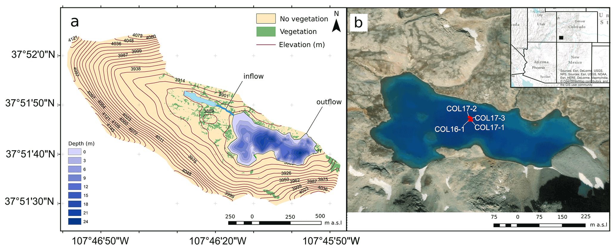
Figure 1 Columbine Lake and its catchment showing the (a) bathymetry and (b) coring location (red circles) in southwestern Colorado (black rectangle in inset map). Vegetation extent for the year 2017 is based on Arcusa et al. (2019a). Image credit: Esri, DigitalGlobe, GeoEye, Earthstar Geographics, CNES/Airbus DS, USDA, USGS, AeroGRID, IGN, and the GIS user community.

3 Methods

3.1 Coring, description, and correlation

Four sediment cores were collected from Columbine Lake at water depths ranging from 21 to 24 m. One 81 cm long core was taken in August 2016 (COL16-1 collected at 22 m depth) using an aquatic corer, and three 125 to 142 cm long cores were collected in September 2017 (COL17-1, COL17-2, and COL17-3 collected at respective depths of 23, 24, and 24 m) using a modified UWITEC percussion coring system. All three 2017 cores captured the undisturbed sediment–water interface, but the 2016 core did not. Cores were split, described, and stored at the Sedimentary Records of Environmental Change Lab at Northern Arizona University. Consistent core stratigraphy and marker layers found in all cores except COL17-1 facilitated visual core cross-correlation (Appendix Fig. A1). All cores except for core COL17-1 are finely laminated, possibly because core CO17-1 was collected on the slope of one of the deep pockets and thus was not considered further in this study.

3.2 Geochronology

This study added three radiocarbon dates to the three previously published by Arcusa et al. (2019a) on cores COL17-3 and COL16-1. Macrofossils of terrestrial plants and aquatic insects were pre-treated using standard acid–base–acid procedures and analyzed for radiocarbon activity on Northern Arizona University's MICADAS equipped with a gas interface system while it was located at the manufacturer's (IonPlus) office in Zurich, Switzerland. Three dates were previously reported by Arcusa et al. (2019a) (UCI 196901, UCI 190157, and UCI 188317) for a mixture of small insects and plant fragments. In addition to radiocarbon, Arcusa et al. (2019a) also measured ²¹⁰Pb and ¹³⁷Cs activities on 20 and 16, respectively, dried and homogenized samples over the top 12.5 cm of core COL17-3 using a Canberra broad energy germanium detector (BEGe; model no. BE3830 P-DET) at the Marine Science Center at Northeastern University.

The radiometric age–depth model was constructed from the concurrent use of the Bayesian modeling R (v4.0.2) software (R Core Team, 2021) packages Bacon (v2.2) (Blaauw and Christen, 2011) and Plum (v0.1.5.1) (Aquino-López et al., 2018). Briefly, Plum is based on a statistical framework, providing more robust and realistic uncertainties when compared to other lead models such as the constant rate of supply (CRS) method (Appleby and Oldfield, 1978). The concurrent use of Bacon and Plum reduces the artificial break in sedimentation rates at the intersection of the ²¹⁰Pb and ¹⁴C ages, and Plum provides a more natural merger of these techniques as it does not require the pre-modeling of the ²¹⁰Pb dates. Additionally, we compare Plum to conventional calculations of CRS (Appleby, 2001) and the constant flux–constant sedimentation (CFCS) method (Krishnaswamy et al., 1971) implemented with the R package SERAC (v0.1.0) (Bruel and Sabatier, 2020).

3.3 Thin sections, sediment imaging, and point measurements

To facilitate investigation, measurement, and delineation of the fine laminations, the sediment was subsampled and impregnated with low-viscosity epoxy resin following a modified approach of Lamoureux (1994). The percentage of epoxy to acetone was increased multiple times before fully embedding the sediment. Overlapping sediment slabs (7.0 cm × 3.0 cm × 1.5 cm) were sampled and placed in an acetone bath for fluid replacement. Acetone was exchanged every 12 h for 5 d until no water was left in the sediment. Following fluid displacement, Spurr's low-viscosity embedding resin was exchanged every 12 h for 3 d and left to cure for 1 d at room temperature followed by 1 d at 40 ^∘C, 1 d at 50 ^∘C, and 1 d at 60 ^∘C. Slabs were cut at the Northern Arizona University machine shop, and sections were sent to Quality Thin Sections in Tucson, AZ, for mounting and polishing. Images of the thin sections were taken at 2× and 10× magnification under polarized light with a petrographic polarizing microscope (Carl Zeiss Axiophot) connected to a digital camera (Carl Zeiss Axiocam) and automated stepping stage (PETROG System, Conwy Valley Systems Ltd, UK). Individual images were stitched into a mosaic using the Stitching plugin (Preibisch et al., 2009) in ImageJ.

3.4 Probabilistic varve chronology

An important distinction exists between laminations and varves, as the term “varve” is usually reserved for annually deposited laminations (Zolitschka et al., 2015), which has been demonstrated in various ways including comparing to radiometric data, observing sedimentation through time using sediment traps, and replicating measurements across multiple cores. This distinction is especially relevant in this study because although the well-laminated sections meet the criteria to be considered varved, most importantly by their agreement with independent radiometric data, a significant portion of the laminations in Columbine Lake sediment are indistinct and do not meet the typical definition of a varve (e.g., Skilak Lake; Boes et al., 2018). The goal of this study, however, is to characterize the probability of the temporal duration of each lamination in a sequence of indistinct and intermittently laminated sediment. To make this distinction clear, we use the term “lamination” to refer to what was observed and delineated in the sediments and the term “varve” to refer to an annually deposited lamination modeled or simulated by our algorithms. Furthermore, as will be described below, the method does not “count” laminations in the traditional sense of an observer counting laminations; the method uses delineations of laminations made by an observer which a model then simulates as a “count”. To quantify uncertainty and ultimately estimate prior probabilities, all our algorithms are run in ensemble. This means that any given observed lamination may be simulated as a varve in some ensembles and not in others. In Sect. 4.6, we argue that the Columbine Lake sequence meets the criteria of a varved sequence, whereas the probability of any given lamination being annual is always < 1.

The data analysis in this study expands on a code base in R called “varveR” (v0.1.0) (McKay and Arcusa, 2021) that builds varve chronologies while quantifying uncertainty due to lamination identification, inter-core differences, and likelihoods of over- and under-counting. varveR is a Bayesian probabilistic algorithm that quantifies age uncertainty by integrating information from the age distribution of marker layers from multiple cores (Fortin et al., 2019). The algorithm follows two concepts. First, it uses the sedimentological understanding of the likelihood of the correct delineation of the laminations such as those related to the ease of distinguishing them. Second, it takes advantage of the replication from the marker layers correlating between cores to quantify the likelihood of under- and over-counting as well as the uncertainty in the total count as a function of depth.

The algorithm's inputs include (1) thicknesses for each lamination for each core, (2) site-specific marker layers to stitch the sections together into a sequence, (3) prior estimates of over- and under-counting, and (4) inter-core marker layers and their prior probabilities. All four inputs are necessary for the code to work. In this study, thickness delineations were created as ArcGIS ArcMap shapefiles (Appendix Fig. A2). We chose this software for convenience, but in the code's next version we will add the possibility to use open-source shapefiles. Core-specific marker layers were identified in the overlap between two adjacent thin sections. Inter-core marker layers were identified in each core using thin sections and core images. Lamination boundaries, core-specific marker layers, and inter-core marker layers were identified independently by three observers working separately, allowing for better quantification for these aspects of uncertainty. All observers were trained to identify lamination structures and to use common protocols to demarcate lamination boundaries, lamination codes, and marker layers in ArcGIS. Prior to this project the observers had minimal experience identifying varves.

The algorithm uses prior likelihoods of over- and under-counting and updates them, if necessary, as it iterates. The prior likelihoods are selected by the operator but may be the difference in the number of laminations delineated by two observers expressed as a percentage and converted into a probability (e.g., Fortin et al., 2019). With each iteration, the only constraint is that the duration across cores between marker layers must be the same. varveR outputs an n-member ensemble of varve counts and thicknesses for each core and a composite of all cores, where n is a user-defined number of iterations. The ensemble is used to quantify the uncertainty in depth as a function of varve year and can be transposed to estimate uncertainty in varve year as a function of depth. The algorithm is completely independent from radiometric age control.

Here, we expand on this algorithm to include information on lamination quality as an indicator of the likelihood of over- and under-counting. Although varve quality indices have been used in past research as a qualitative aid to interpretation (Bonk et al., 2015; Dräger et al., 2017; Żarczyński et al., 2018), here we integrate this information quantitatively. Each lamination was assigned one of six different codes (Appendix Fig. A2) with a corresponding distribution of over- and under-counting prior probability estimate (Sect. 3.5). Codes 1, 2, and 3 are assigned by the clarity of the lamination's appearance, with a code value of 1 being of higher clarity than a code value of 3. A code of 4 was used when it was difficult to distinguish whether two couplets represented 1 year with sub-laminae or 2 separate years. In this case, they were delineated as two laminations and denoted with a code of 4, which were assigned a 50 % probability of over-counting.

Distinctly laminated sediments interspersed with indistinctly laminated sections comprised zones up to 2 cm thick with weak to absent laminations (Appendix Fig. A2). These indistinct sections were relatively common, comprising 8.7 %–19.6 % of the total sediment thickness across observers. For these sections, a code of 5 was assigned. In addition, sections with sediment missing from what could be deemed technical reasons (e.g., between two adjacent thin sections without overlap or in gaps created by breakage during the embedding process) were assigned a code of 6. Previous studies have addressed the issue of indistinct sections or missing laminae by either interpolating sedimentation rates from nearby varved segments (e.g., Hughen et al., 2004) or using the probability distribution of the varves' seasonal layers to derive sedimentation rates (Schlolaut et al., 2012). These approaches did not work for us because our Bayesian modeling approach requires an estimate of varve thicknesses for each year rather than an estimate of mean sedimentation rate or missing time. Therefore, to simulate varves in indistinct (or missing) intervals, we developed an emulator that randomly chooses a distinctly laminated section of the core and with a length of that section matches the thickness of the interval as nearly as possible. Because laminations at Columbine Lake are very thin (typically <0.5 mm) relative to the thickness of the indistinct intervals (typically ∼ 4 mm), this procedure alone matches the cumulative depth closely. Subsequently, a minute thickness adjustment is applied across the sequence to ensure a perfect match in total thickness and conservation of the depth of the core. This approach assumes that the sedimentation processes in these intervals are consistent with the well-laminated sections and other laminated intervals can serve as surrogates for indistinct sections. We argue that this assumption is valid for Columbine Lake, as the distribution of the lamination thickness is similar in both cores throughout the sections with distinct laminations (Appendix Fig. A3). Furthermore, there is no evidence for systematic changes in the mode of deposition in these sections, as the indistinct sections occur throughout both cores, but not always in the same intervals, and the sedimentary features were mostly the same above and below the indistinct sections, suggesting that the indistinct laminations are due to changes in preservation, not the sedimentation process.

3.5 Varve modeling

The modified varveR algorithm, which we will refer to as our “varve-only” model, was used to build two varve chronologies, each following a different scenario. In both scenarios, codes 1, 2, and 3 were given over- and under-counting priors, code 4 was given a 50 % chance of over-counting and a 0 % chance of under-counting, and codes 5 and 6 were simulated using the emulator as described above. Both scenarios treated codes 4–6 the same and only codes 1–3 changed. In the first scenario, the priors for codes 1–3 were symmetrical and based on values found in the literature (Fig. 2a, e.g., Dräger et al., 2017). This produced a chronology that would resemble the conventional varve chronology construction and allow for comparison. However, due to missing or indistinct varves, varve chronologies are often subject to under-counting (Tian et al., 2005; Żarczyński et al., 2018). Because the laminations in Columbine Lake are thin and lack clarity in their appearance, a prior shifted towards under-counting may be more realistic for lamination code 2. The laminae associated with lamination code 3 are indistinct, and we have no reasonable a priori estimates of over- or under-counting probabilities. To accommodate these informed priors, in the second scenario we assigned wider symmetrical priors for code 1, wide and asymmetrical priors for code 2, and an uninformed prior for code 3 (Fig. 2b). This expanded algorithm incorporates uncertainty pertinent to lamination quality, inter-core variation, and expert judgment (Fig. 3).

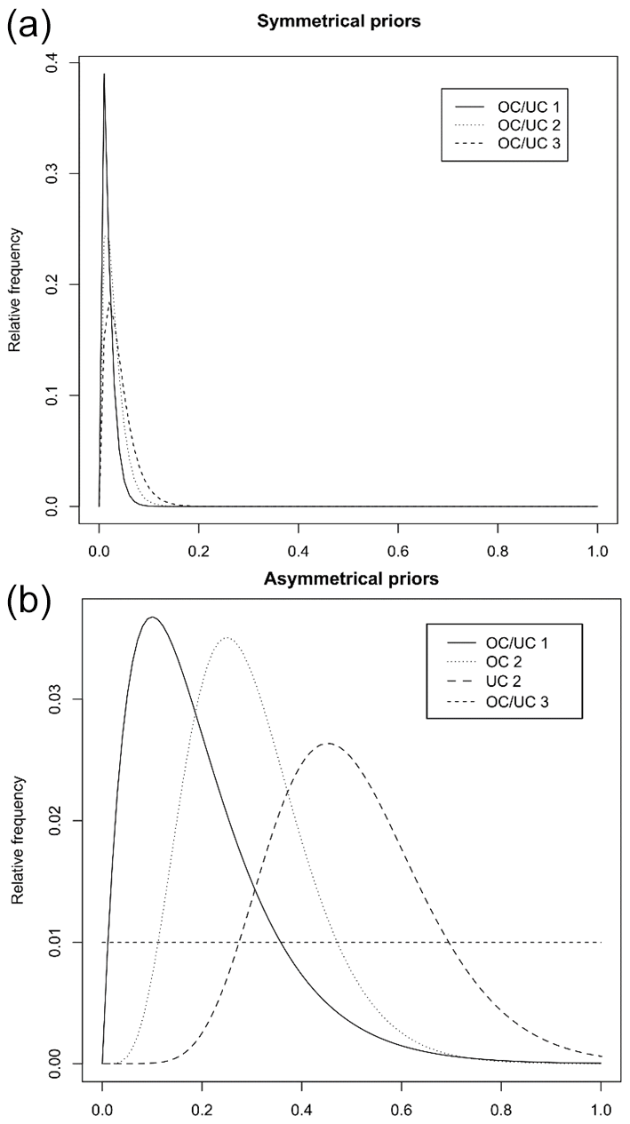
Figure 2 Lamination quality codes and their associated under- (UC) and over-counting (OC) gamma distribution priors for (a) symmetrical and (b) asymmetrical priors.

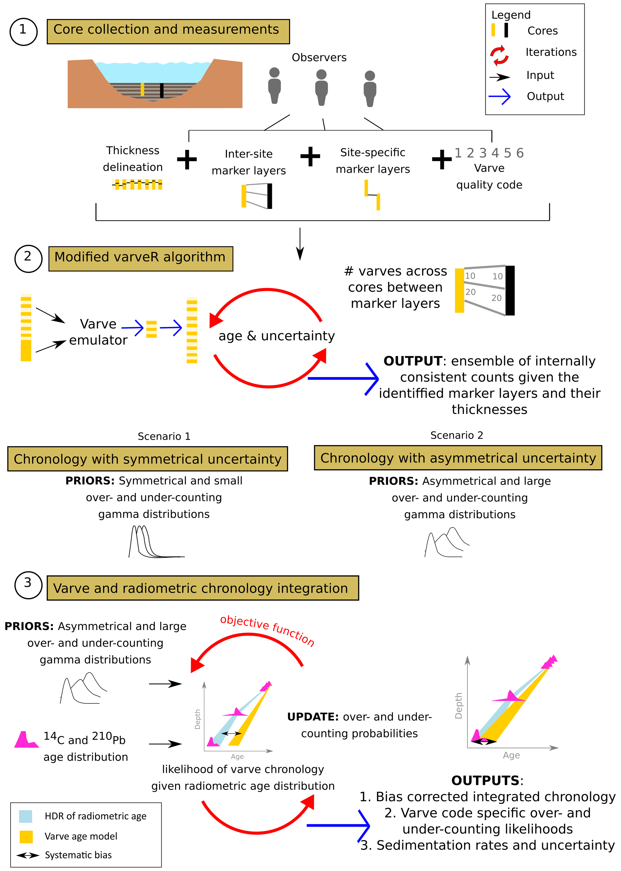
Figure 3 Schematic of the approach used in this study. (1) Gathering raw measurements of lamination thickness, counts, and marker layers for each core and each observer. (2) Using our varve-only model to produce a chronology following scenario 1 (symmetrical and literature-derived likelihoods of over- and under-counting) and scenario 2 (asymmetrical and larger likelihoods of over- and under-counting). (3) Integrating radiometric information into the varve chronology by updating the prior likelihoods of over- and under-counting in an objective function. The posteriors of the nth best function output are used to run an updated varve-only model and produce the final chronology that minimizes systematic bias, quantifies uncertainty related to misidentifying marker layers, observer bias, and lamination quality, and outputs sedimentation rates with uncertainty.

3.6 Varve and radiometric chronology integration

Bayesian statistics provide the opportunity to combine different chronological data and their uncertainty (e.g., Buck et al., 2003) as well as information regarding the sedimentation process (e.g., Blockley et al., 2008) by informing priors (Brauer et al., 2014). Here we use Bayesian learning to update prior estimates of the counting uncertainties for each observer given the constraints from the independent radiometric age–depth model. Then, we combine the model produced from each observer into one chronology.

Our Bayesian framework uses a custom Gibbs sampler to estimate posterior distributions of over- and under-counting probabilities for each lamination code. The Gibbs sampler is initialized using the prior estimates of over- and under-counting used in the asymmetrical varve-only model (Fig. 2b). The sampler updates using an objective function that calculates the likelihood of a proposed varve chronology given the radiometric ages and their probability distributions. We assume that the probabilities associated with lamination quality codes 1 and 2 are best described using gamma distributions and must fall between 0 and 1. For algorithmic efficiency, we loosely impose the assumption that proposed adjustments that increase over-counting rates should be balanced by decreases in under-counting rates, although overall reductions in both over- and under-counting are possible and do occur. We ran the Bayesian algorithm independently for each of the three observers until the objective values stabilized (∼ 100 iterations), then removed the burn-in and thinned the parameter chain to keep 1000 values. Finally, for each observer, we select the parameters corresponding to the 300 highest objective values and combine them into combined posterior distributions. These posterior distributions on the counting rates are used to calculate an ensemble of updated varve counts and produce a master chronology that effectively combines the radiometric age–depth model and the lamination measurements from all observers (Fig. 3), which we will refer to as the “multiple observer integrated model (MOIM)”.

3.7 Varve chronology verification

A varve-based age–depth determination must be cross-checked with other independent dating methods to (1) support the interpretation of laminations as annual and (2) to identify systematic errors (Ojala et al., 2012; Zolitschka et al., 2015). As discussed in Sect. 3.4, we do not aim to verify that all the observed laminae are annual, rather that our model represents an annually laminated depositional regime with appropriate uncertainties. To do this, we examine our varve-only and integrated model outputs as age–depth curves. Then, the near-surface counts are compared to radionuclide-based (¹³⁷Cs and ²¹⁰Pb) age–depth models that use conventional CRS, CFCS, or Plum (Sect. 3.2). The full sequence is compared to a Bayesian radiocarbon age–depth model. All comparisons are made using the dated core COL17-3.

4 Results

4.1 Sediment profile

Columbine Lake sediments were previously described generally by Arcusa et al. (2019a), and more detail is provided here. The sediments are composed of minerogenic, laminated silts and clays ranging in color from grey to reddish-brown to orange (Fig. 4a). Three of the four cores showed identical sediment profiles, meeting the requirement of reproducibility, but only COL17-2 and COL17-3 captured an intact sediment–water interface and laminations (Appendix Fig. A1). Sediment between 141 and 126 cm (core depths from COL17-2) are characterized by massive grey clay-sized sediment. Sediment between 123 and 72 cm contains poor-quality laminations frequently interspersed with indistinct sections. The sections of indistinct lamina preservation generally correlate across the parallel cores, although they are more prevalent in core COL17-2 (Fig. 4a). Sediment between 72 and 12 cm contains laminations of average clarity with indistinct sections (Fig. 4a). Sediment between 12 and 0 cm contains well-defined laminations and massive fine silt layers. The lower part (12–2 cm) contains fine and grey laminae interspersed by two massive layers. The two massive light brown layers are both in core COL17-2, with core COL17-3 only containing the youngest of the two. Core COL17-3 contains a layer of indistinct laminations that cross-correlates with the oldest of the two COL17-2 massive layers, suggesting the layers are composed of poorly preserved lamina as opposed to a single massive bed deposited rapidly. The upper part (0–2 cm) contains thicker bright orange lamina just below the sediment–water interface.

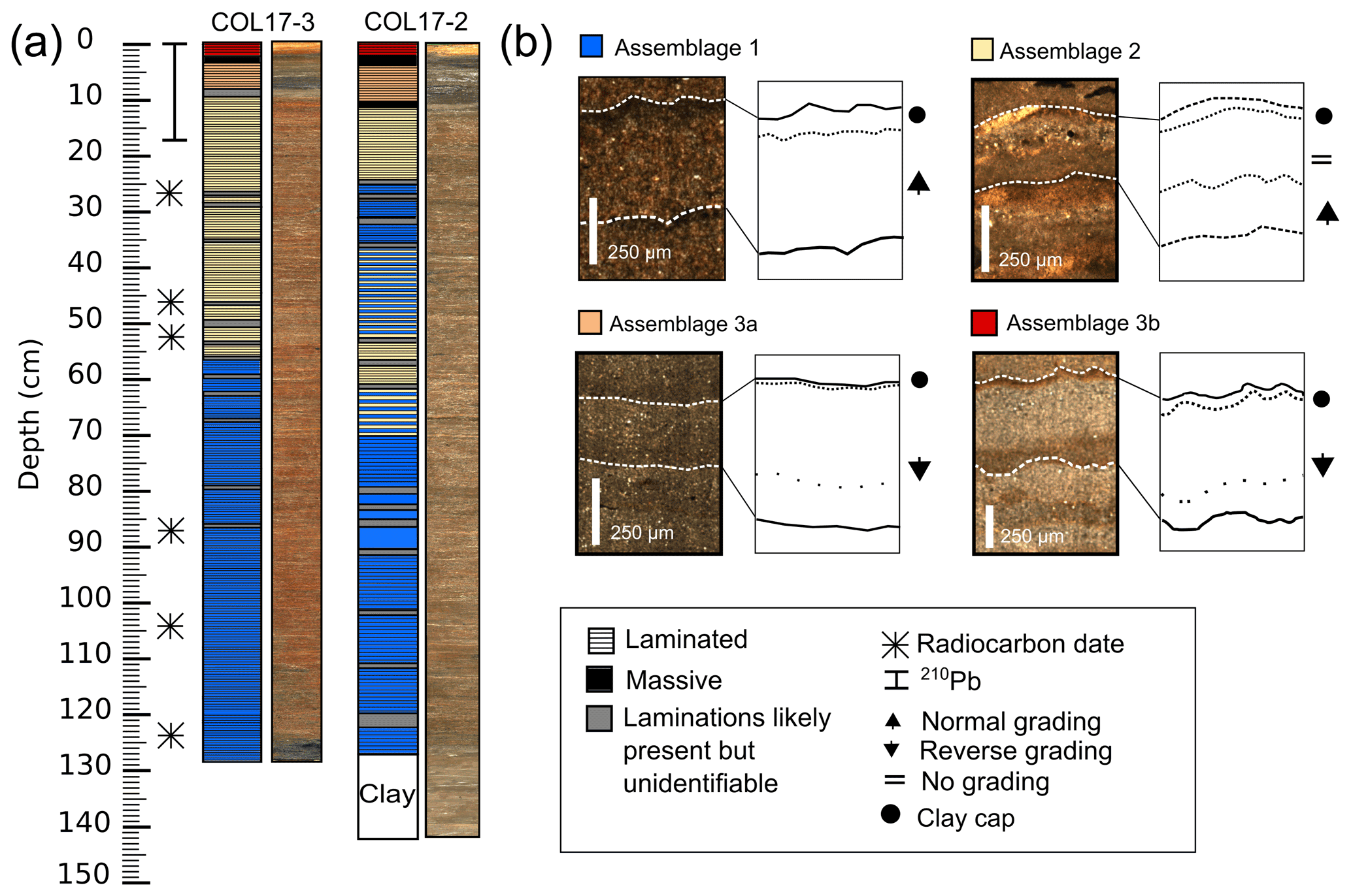
Figure 4 Sediment and lamination profiles. (a) Lithostratigraphy and location of radiometric samples of cores COL17-3 and COL17-2. Images are true color. The base of COL17-3 is black because the oxidized red crust has been scraped off. (b) Microscopic thin section examples of assemblages 1, 2, and 3.

4.2 Lamination description

The examination of thin sections revealed complex microfacies that repeat within each lamination, indicative of a rhythmic change in the depositional environment. Moreover, comparison to radiometric measurements demonstrates that this rhythmic layering is annual (Sect. 4.6). Therefore, the sediment is described here as true non-glacial clastic lamina (Zolitschka et al., 2015). Three assemblages of clastic lamina are further subdivided based on their internal structure (Fig. 4b). Assemblage 1 is composed of typical couplets of silt and clay, assemblage 2 couplets are interrupted by a third coarser-grained sub-laminae, and assemblage 3 couplets are inversely graded, with thinner (3a) or thicker (3b) clay-sized caps and darker (3a) or lighter (3b) laminae (Fig. 4b).

4.2.1 Assemblage 1

Assemblage 1, most common in the deepest half of the sequence, consists of couplets identified by color and grain size. The bottom lamina is characterized by ungraded or fining-upward grading of light reddish-brown sediment (Fig. 4b). The top lamina is a fine-grained, dark brown clay-rich cap (Fig. 4b). The contact between them is generally sharp.

4.2.2 Assemblage 2

Assemblage 2 is most common in the top half of the sequence. Like assemblage 1, assemblage 2 bottom lamina is silt-sized and inversely graded. The top lamina is terminated with a dark reddish-brown clay-sized cap. However, the couplets are often interrupted by coarser-grained matrix-supported laminae, which are composed of plagioclase, quartz, and oxides, as identified under polarized microscope light. The contact between the bottom lamina and this lamina is erosional.

4.2.3 Assemblage 3

Assemblage 3 is found exclusively at the topmost part of the sequence and can be subdivided into assemblage 3a and 3b. The deeper of the two in the sediment sequence, assemblage 3a, is thicker and contains a reverse grading of fine and dark grains at the bottom to coarse and light sediment at the top (Fig. 4b). This lamina is followed by a thin and sometimes nonexistent clay-sized cap. Finally, at the topmost part of the sediment sequence is assemblage 3b, similar in composition to assemblage 3a. The difference is a strongly pronounced clay-sized cap. Both assemblage 3a and b have a sharp change in color from dark to light. Assemblage 3 differs from assemblage 2 by its reverse grading.

4.3 Counts, thicknesses, and quality

Lamination thicknesses, excluding laminae of quality codes 4, 5, and 6, are similar for each core (Table 1), with a combined mean and standard deviation of 0.5 ± 0.3 mm. Thicker laminae were found in COL17-3 (4.5 mm) compared to COL17-2 (2.81 mm). Lamination quality varied between observers and fluctuated between moderate and poor quality throughout (Fig. 5). The minimum thicknesses of 0.04 mm measured in COL17-2 may appear small, but the algorithm does not allow a value smaller than any measurement.

Table 1 Summary statistics based on the average of all observers' measurements, excluding intervals of indistinct laminations. Total varve counts indicate output of the symmetrical varve-only model.

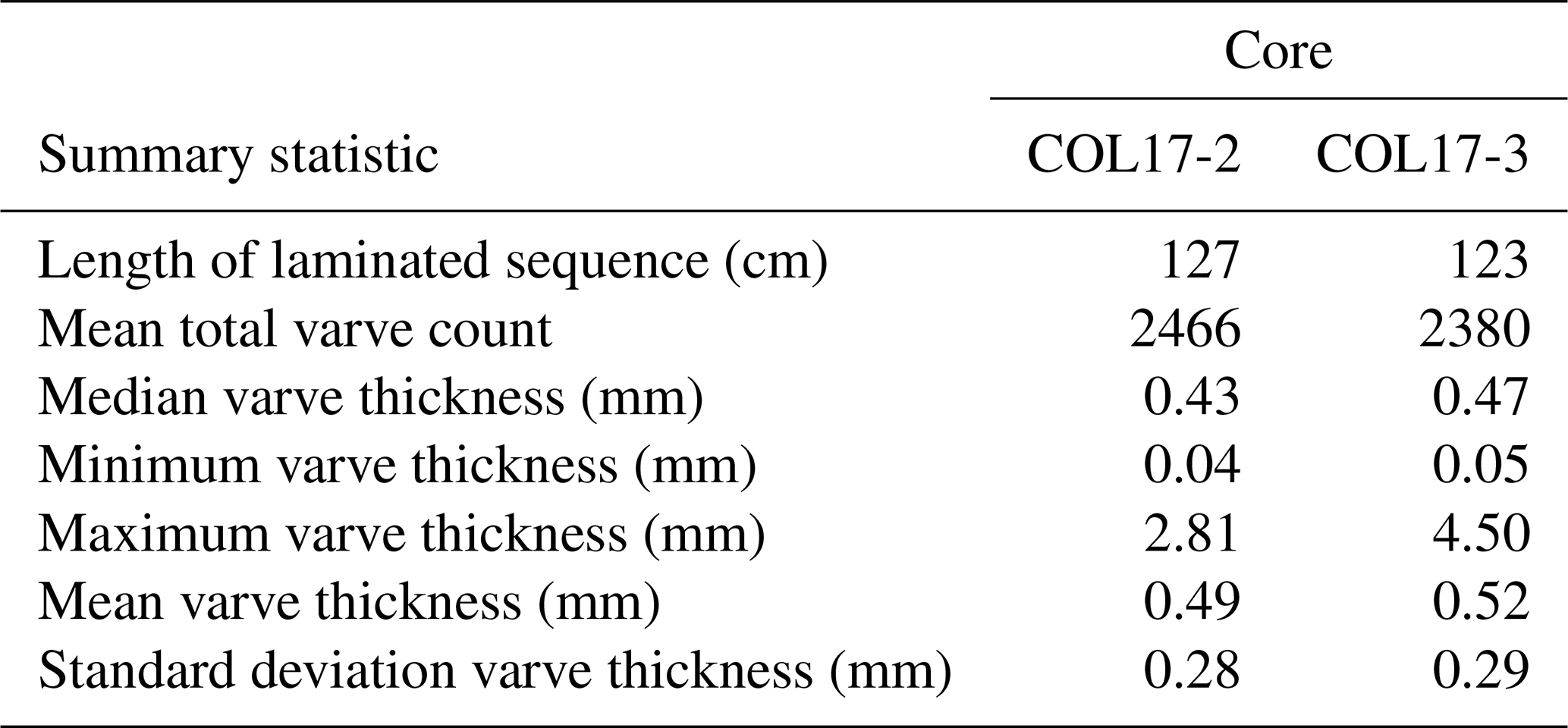
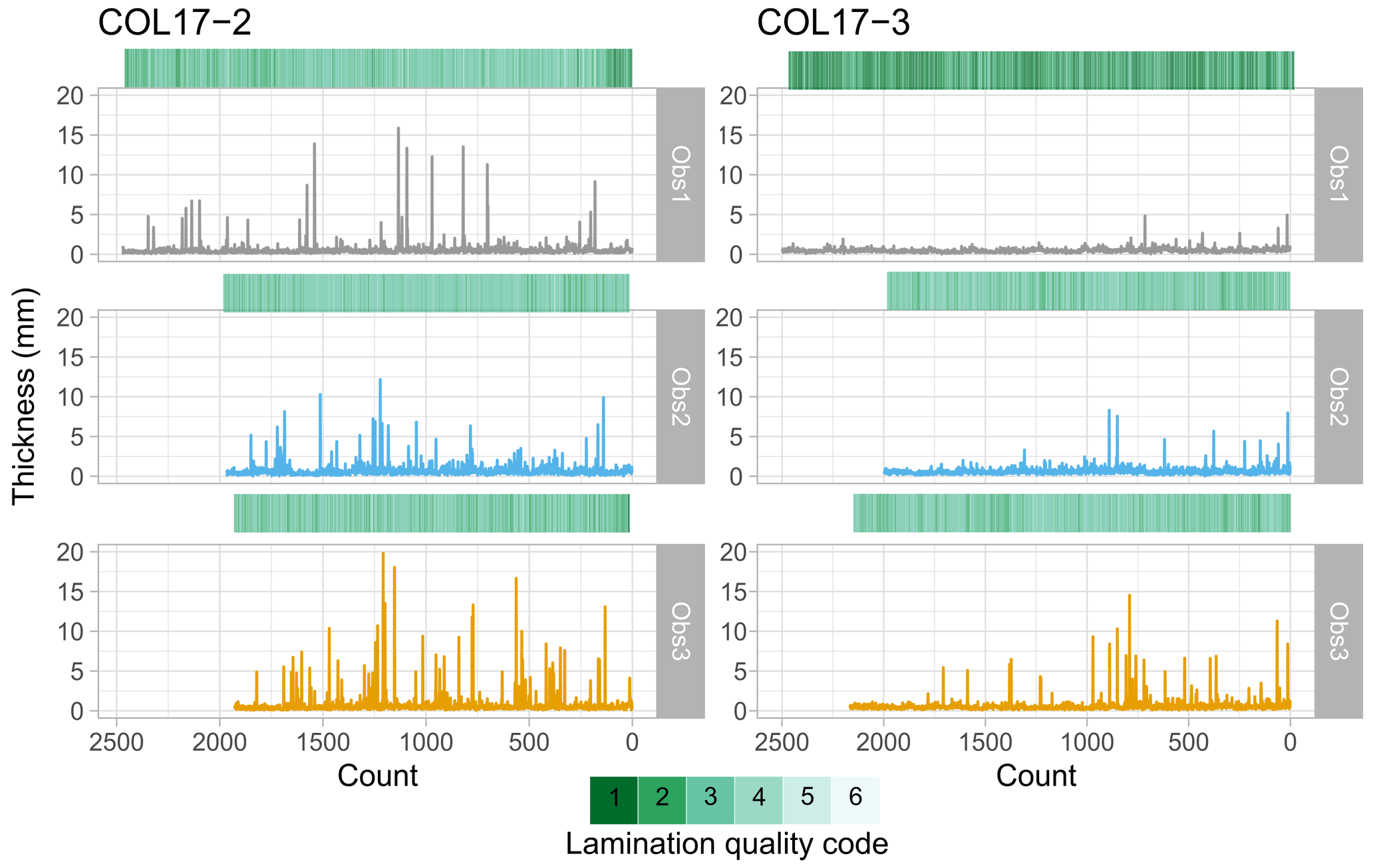
Figure 5 Observer measurements of lamination thicknesses (lines) and quality (heat maps) for cores COL17-2 and COL17-3.

Table 2 Comparison of observer- and core-specific varve ages based on the symmetric and asymmetric varve-only model as well as the integrated model. HDR: highest probability density region.​​​​​​​

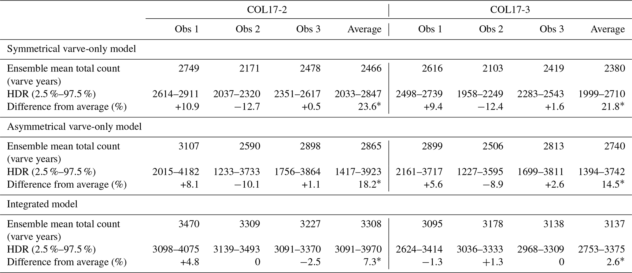
^∗ Indicates the observer agreement as the range in the percentage difference from the mean.

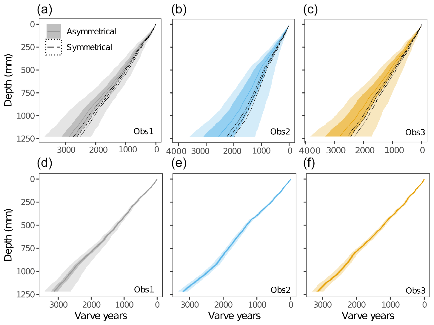
Figure 6 Comparison of varve-only modeled counts by (a, d) observer 1, (b, e) observer 2, and (c, f) observer 3 for dated core COL17-3. In the top row, the modeled varve counts are shown when using symmetrical (dotted envelop) and asymmetrical (shaded envelop) priors. For the symmetrical uncertainty, the median (dashed line) and the 97.5 % (dotted region) high-density regions are depicted. For the asymmetrical uncertainty, the median (darkest line), 75 % (darkest shaded region), and 97.5 % (lightest shaded region) high-density regions are depicted. In the bottom row, the integrated varve and radiometric models are shown.

Lamination observations were integrated into a varve count ensemble using the varve-only model. With the symmetrical varve-only model, cores COL17-2 and COL17-3 contain a total of 2466 (highest probability density region: 2075–2880) and 2380 (1999–2710) varves, respectively (Table 2, Fig. 6). This amounts to a cumulative uncertainty of −391 to +414 varves (−17 % to +15 %) for COL17-2 and −381 to +330 (−17 % to +13 %) for COL17-3. With the asymmetrical varve-only model, the mean total varve count increases by 300–400 varves to 2865 (1417–3923) for COL17-2 and 2740 (1394–3742) for COL17-3, although the cumulative uncertainty also increases to −1448 to +1058 varves (−68 % to +31 %) and −1346 to +1002 varves (−65 % to +31 %), respectively.

4.4 Observer-related uncertainty

Three observers independently delineated the laminae of cores COL17-2 and COL17-3 in one transect each (Appendix Fig. A2). The cumulative uncertainty of each observer to the mean was higher for the asymmetrical than symmetrical varve-only model. The uncertainty varied between 0.5 % (observer 3 COL17-2) and 12.7 % (observer 2 COL17-2). The asymmetrical varve-only model suggests more under-counting for observers 2 and 3 and more over-counting for observer 1 (Fig. 6). However, segment differences are both positive and negative for all observers, indicating that systematic bias may not be an issue (Appendix Table A1). The observer agreement is high for minimum thickness but low for maximum thickness (Appendix Table A2). Observers disagreed on the number of indistinct sections, pointing to the subjectivity of varve delineations and confidence levels. Agreement on varve quality between observers is low (Fig. 5), highlighting the challenge of identifying laminae in some sections of the sequence and indicating further subjectivity. Sections with thicker varves generally correlate across all observers such as between the varve years of 0–100 and 750–1000 in COL17–3 or between the varve years of 1000–1500 in COL17-2 (Fig. 5).

4.5 Marker layer uncertainty

As marker layers were assigned by each observer individually, they do not always agree between observers. The identification of marker layers is a key additional source of uncertainty that is modeled in our approach. Consequently, the varve counts between marker layers, or segment counts, in each core indicate a combination of inter-core variability due to the sediment quality and observer judgment (Appendix Table A1). The largest segment difference was 110 % (172 years) for one observer, which cannot be explained by marker layer misidentification alone. Instead, it indicates that one observer identified more indistinct sections than the other observers for one of the sites.

4.6 Independent validation

The topmost part of core COL17-3 was dated with two independent radionuclide profiles. The ²¹⁰Pb activity in Columbine Lake exhibits a gradual downcore decline that reaches equilibrium around 50 Bq kg⁻¹ below 8 cm (Fig. 7a). The age at the base of the radionuclide measurements (12 cm) modeled by conventional methods for CRS and CFCS varies widely (Fig. 7c): CRS reaches 1883 ± 14 CE, whereas CFCS comes to 1940 ± 13 CE. In comparison, the Bayesian solution has a wider but likely more realistic uncertainty at 12 cm, yielding a median age of 1784 CE with a 95 % highest-density region of 1866–1679 CE. Although the range of the uncertainty is more realistic, the ages themselves may not be: Pb becomes unsupported at 8 cm depth (∼ 1800 CE). The ¹³⁷Cs activity shows a single peak at 3.25 cm (Fig. 7b), which we attribute to the 1963 CE fallout from nuclear weapon testing. The peak's depth appears to be younger by 20 to 30 years in the ages modeled from the ²¹⁰Pb profile: CRS indicates 1996 CE, which for CFCS it is 1998 CE and 1984 CE for Plum. Despite this discrepancy, it is very unlikely that the peak at 3.25 cm is related to Chernobyl fallout; such a peak is almost never found in North America (Lima et al., 2005; Omelchenko et al., 2005; Munoz et al., 2019), and we are not aware of a Chernobyl-related ¹³⁷Cs peak reported in lake sediment in the western United States. It is more likely that the ²¹⁰Pb profile is incorrect than the ¹³⁷Cs peak being attributed to Chernobyl.

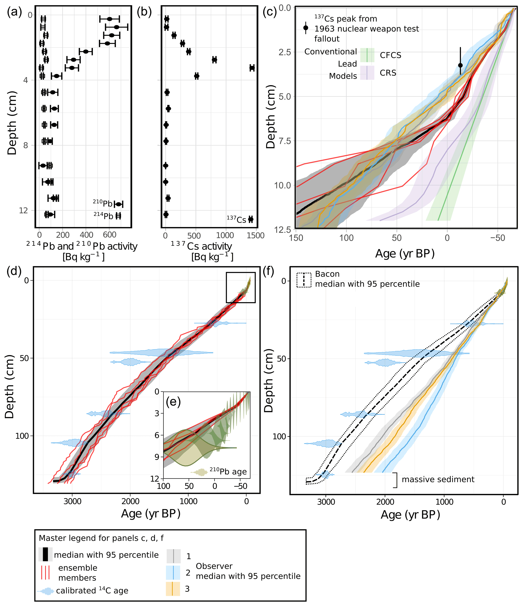
Figure 7 The chronology of Columbine Lake core COL17-3. (a) ²¹⁰Pb raw measurements. (b) ¹³⁷Cs raw measurements. (c) Comparison of lead models (green: CFCS, purple: CRS) and the caesium peak of the 1963 nuclear weapon test to the radiometric model (black, red, grey: Plum and Bacon) and to the varve-only model (light grey, blue, yellow: varve-only model). (d) Radiometric model produced from combining the Bacon-derived radiocarbon age–depth model with the Plum-derived lead age–depth model. Black and grey represent the median age with 95th percentile. The red lines represent five randomly selected ensemble members. Blue probability distribution functions represent the calibrated radiocarbon ages. (e) Plum-derived lead age–depth model. Brown probability distribution functions represent the sampled ²¹⁰Pb ages. (f) Comparison of the radiometric model (Bacon and Plum combined) to the varve-only models for each observer. Panel (c) shows the same area of the graph as panel (e).

Table 3 Uncalibrated and calibrated radiocarbon dates.

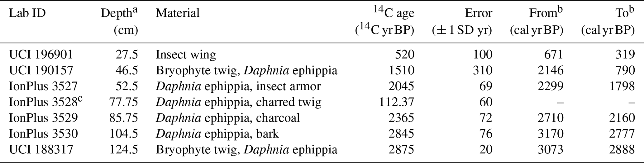
^a Mid-point depth of 1 cm thick sample. ^b Two-sigma range calibrated with IntCal20 curve. ^c Value is given in percent modern carbon (fraction modern multiplied by 100). Fraction modern for this sample is 1.1237. This date was not used because it returned a modern age.

A total of six radiocarbon dates ranging in age from 20 to 310 years were used to model the age profile of Columbine Lake sediment (Table 3). One new date was discarded as it returned a modern age (IonPlus 3528). Two more dates (IonPlus 3529 and IonPlus 3530) were measured on a mixture of plant fragments, bark, and aquatic insects due to the paucity of organic material found in the sediment. The uncertainty of the two new dates ranged from 72 to 76 years. The calibrated basal age at 124.5 cm is 2997 yr BP (95.4 % probability: 3073–2888).

To verify the annual nature of the couplets in Columbine Lake, we compare the topmost part of the varve-only model with symmetrical priors to the ¹³⁷Cs peak and the entire sequence to the radiocarbon profile (Fig. 7c and f). Cesium-137 is used for comparison because of its lower uncertainty as opposed to the ²¹⁰Pb age models, which are not in close agreement among themselves. The varve count and uncertainty by all three observers show high agreement with the ¹³⁷Cs peak, suggesting that the couplets are annual. The whole sequence agrees well with the radiocarbon profile, particularly in the top 25 cm. Uncertainty surrounding the varve count increases downcore, and the varve counts no longer overlap with the radiocarbon uncertainty below 50 cm. The basal radiocarbon age is older than the mean age estimated by both symmetrical and asymmetrical varve-only models by 600 and 250 years, respectively. The cumulative uncertainty of the asymmetrical varve-only model encompasses the radiocarbon basal age, whereas the symmetrical varve-only model does not. The radiocarbon age estimate is the closest to the estimate from observer 1. The comparison with radiocarbon also serves to identify systematic biases. In the case of Columbine Lake, the ¹⁴C data suggest that the varves are systematically under-identified.

4.7 Varve and radiometric data integrated model

One integrated model was created for each observer. The integrated models updated the prior estimates of the counting uncertainties given the constraints from the independent age model and given each observer's varve thicknesses, varve quality designation, and marker layer identification. The models sampled the probability space for 50 000 iterations, and the burn-in occurred rapidly in < 100 steps (Appendix Fig. A4). The integrated models result in similar cumulative uncertainty as the symmetrical varve-only model but much smaller than the uncertainty estimated by the asymmetrical varve-only model (Figs. 6 and 8). The integrated models also converge more: the difference in the basal age between observers shrinks to 2.6 %, down from 21.8 % in the symmetrical varve-only model. The posterior likelihoods of over- and under-counting are larger than the symmetrical priors (Fig. 2 compared to Appendix Fig. A5). They also varied with each varve quality code and with each observer (Appendix Fig. A5). The integrated models were more successful at correcting for over- and under-counting for observers 2 and 3 than observer 1 as seen from the more symmetrical cumulative uncertainty for those observers (Appendix Fig. A4).

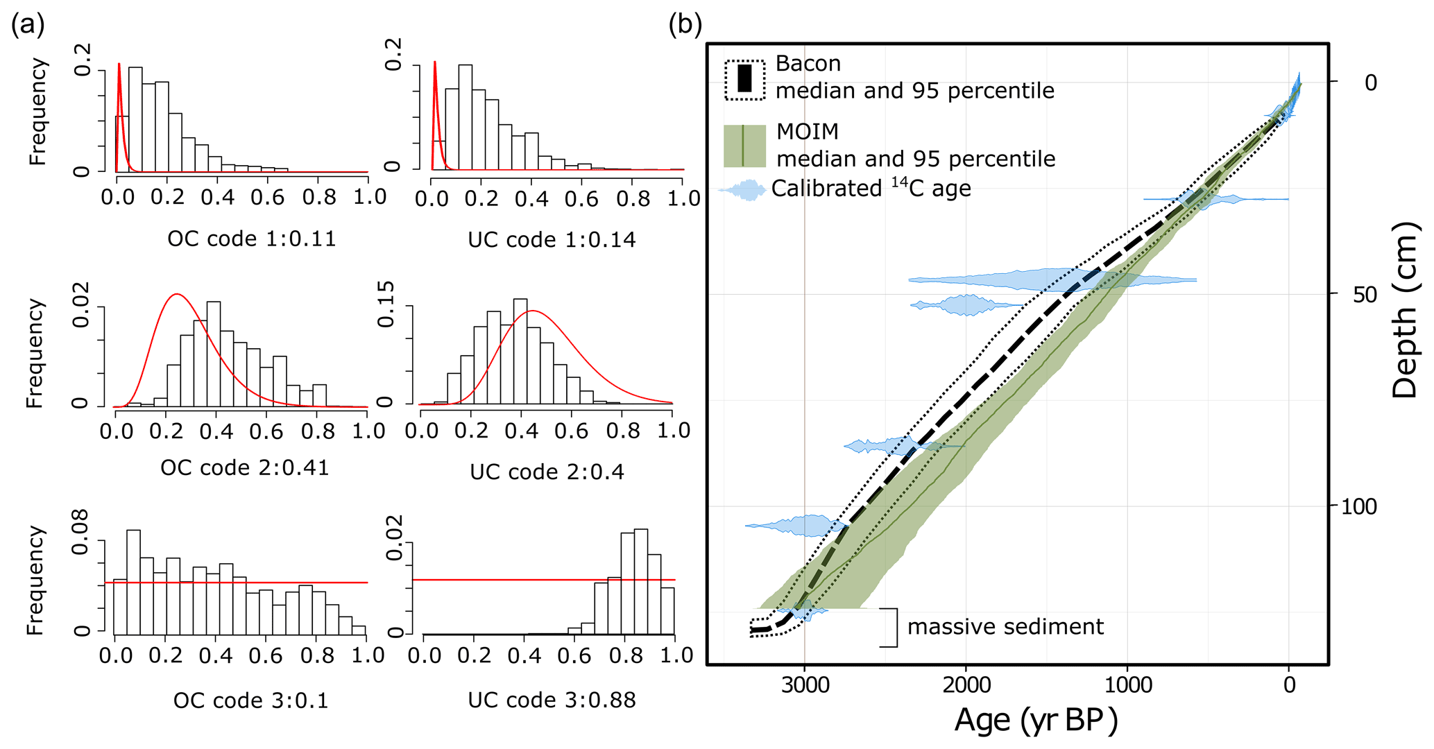
Figure 8 Integrated varve–radiometric model. (a) Over- and under-counting posterior distributions for the multiple observer integrated model (MOIM) for each lamination quality code (1, 2, 3). (b) Age–depth model comparison of the independent (Bacon) age model and the multiple observer integrated model. OC: over-counting. UC: under-counting. The red line indicates the prior distributions.

Each observer's integrated model was combined into one single integrated model, referred to as the multiple observer integrated model (MOIM). The MOIM's cumulative age extends to 3137 (3375–2753) varve years or 1120 BCE (1358–736 BCE), corresponding to a cumulative uncertainty of −384 to +238 years (−13 % to +7 %) (Table 2). The cumulative mean age is older than the symmetrical and asymmetrical varve-only models as well as the independent model. However, the HDR encapsulates the mean age of the radiometric model (Fig. 8b). The greatest deviation between the independent model and the MOIM occurs between 30 and 80 cm depth where indistinct sections are most frequent (Fig. 8b). The cumulative uncertainty in the MOIM is lower than the asymmetrical varve-only model and similar to the symmetrical varve-only model.

The posterior probabilities of over- and under-counting consistently increase for lamination quality codes 1 and 2, consistent with the priors and theory, as we would expect the highest-quality lamina to be identified correctly most frequently. The posterior probabilities of under- or over-counting are higher than the priors for all lamination quality codes except for the probability of under-counting code 2 (Fig. 8a). The probability of over- and under-counting is similar for varve code 1, with a slight tendency for more under-counting (11 % vs. 14 %). Furthermore, the probability of over- and under-counting varve code 2 is the same (41 % vs. 40 %). In contrast, the likelihood of over-counting varve code 3 is much smaller than the likelihood of under-counting (10 % vs. 88 %). However, the distribution of the likelihood of over-counting is much wider than for other lamination quality codes, indicating that this parameter has the least influence on the iterative improvements made by the Gibbs sampler. More under-counting appears with deeper sediment due to the dominance of poorly preserved sediment identified as lamination quality code 3. Similar posterior probabilities resulted from re-running the MOIM with smaller asymmetrical uncertainty.

4.8 Sedimentation rates

The estimated sedimentation rate and its uncertainty varied by method and observer (Fig. 9a). Average rates are similar for all varve-only models with estimates of 0.51 mm yr⁻¹ (HDR: 0.12–1.45) in the symmetrical varve-only model, 0.44 mm yr⁻¹ (HDR: 0.08–1.76) in the asymmetrical varve-only model, and 0.42 mm yr⁻¹ (HDR: 0.08–1.30) in the MOIM. The long-term sedimentation rates from the independent model are similar (0.41 mm yr⁻¹, HDR: 0.39–0.43). In detail, because of the way sedimentation rates are calculated by the program Bacon, the time increments vary, leading to the higher mean sedimentation rate on average evident in Fig. 9. The summary of sedimentation rates shows consistent multimodal distributions for all models and all observers (Fig. 9a). However, no such modes are observed from the raw measurements (Appendix Fig. A3), suggesting that this is a feature that appeared during the modeling. They may represent different modes of sediment deposition or artifacts, but further investigation would be necessary.

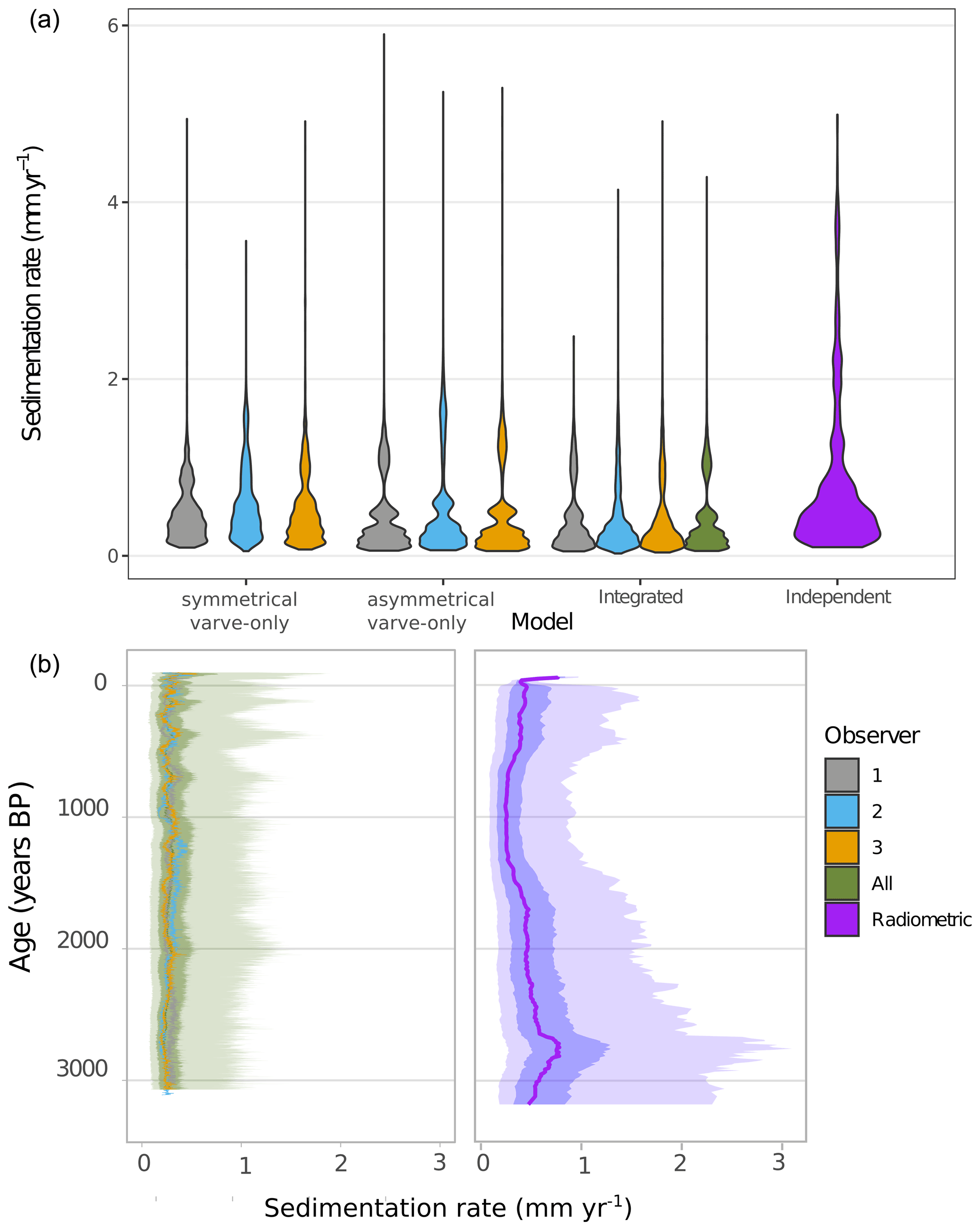
Figure 9 Comparison of sedimentation rates. (a) Summary of sedimentation rates calculated with different models and separated by observer. In green, the multiple observer integrated model (MOIM) is labeled “all”. (b) Late Holocene median (thick lines), 75 % (darker shading), and 97.5 % (lighter shading) highest probability density region estimates of sedimentation rates calculated by the integrated (left) and radiometric (right) models for the dated core COL17-3. Note that the medians for each observer are plotted in the left panel (thick lines).

Sedimentation rates appear to be more stable throughout the late Holocene in the MOIM than for the radiometric model (Fig. 9b). Periods of higher sedimentation rates occur in the MOIM in the last 100 years, 400–500 BP, and 2000–2200 BP. Only the last 100 years of the MOIM show a similar (although subdued) trend as the radiometric model. Although there are significant discrepancies in implied sedimentation rates between different observers in the MOIM, the impact of observer differences on the chronology is far less than in either varve-only model (Fig. 9; Appendix Fig. A6). As expected, the unifying influence of the radiometric dates reduces the impact of observer biases, a potential benefit of the approach, especially in sequences that are difficult to delineate and prone to observer bias.

5 Discussion

5.1 Sources and quantification of uncertainty

Varve chronologies have uncertainties that stem from complex internal structures, poor quality, technical problems, rapid deposition events, and erosion (Ojala et al., 2012). Unlike other sedimentary chronologies, the errors in varve chronologies are propagated by the observer(s), who subjectively determine what is a varve by “lumping” or “splitting” thicknesses. The sources of uncertainty and their quantification in Columbine Lake are now discussed in turn.

5.1.1 Sediment microstructures

The combination of the complex internal structure, shifting structures through time, and thinness of Columbine Lake varves was likely the most important source of uncertainty (Sect. 4.2). The complex sub-lamina internal structures of the clastic varves are the primary cause of the large uncertainties in observer identification and delineation. It is also likely that laminations are missing due to erosion. Both would result in the under-counting that is particularly evident when comparing the symmetrical and asymmetrical varve-only models to the independent chronology (Figs. 6 and 7). The systematic bias is corrected by the MOIM. Additionally, uncertainty in the varve delineation impacts the thickness measurements, which propagates into the sedimentation rates (Fig. 9). At an average thickness of 0.5 ± 0.05 mm, the uncertainty surrounding the delineation of each varve is likely to be proportionately large because of the image quality and pixel resolution used in this study. Missing laminations and misinterpretation due to complex varve structures are common reasons for imprecision (Ojala et al., 2012).

5.1.2 Sediment quality

Closely intertwined with the sediment microstructures, sediment quality is likely the second-most important source of uncertainty in the chronology as seen from the prevalence of poor varve quality codes (2 and 3) (Fig. 5). About 78 % of the sediment of COL17-2 and COL17-3 was identified as code 2, 3, or 4, with all three designations indicating that the observer was less than 80 % certain that the thickness delineated was accurate. We report a cumulative uncertainty (−13 % to +7 %) in the MOIM that is on the higher end of values reported in the literature: a cumulative uncertainty of ± 1 %–3 % is reported in the literature for well-preserved sediment (Ojala et al., 2012) and up to 15 % for unclear, partially disturbed varves in otherwise well-preserved varve sequences (Ojala and Tiljander, 2003; Tian et al., 2005). We also find high estimates of probabilities of over- and under-counting. These uncertainties are not always quantified in the literature, but Ojala and Tiljander (2003) report uncertainties within sections that reach 12 % and indicate more over-counting with depth. Additionally, Fortin et al. (2019) report over- and under-counting estimates of 21.9 % and 14.5 %. We find large uncertainty estimates even for the best-quality varves in Columbine Lake.

The presence of indistinctly laminated sections was frequently identified in both cores (Fig. 4). The timing of these segments is generally correlated across both cores, with exceptions, suggesting a combination of macroscale and microscale processes. We accounted for this uncertainty through varve code 5 by emulating varved sediment. Through this analysis, we found that, on average, more sediment was identified as indistinctly laminated in COL17-2 (25 cm) than COL17-3 (11 cm). In more detail, the identification and thickness of these segments varied between observers, suggesting differences in expert confidence and indicating that high uncertainty may surround the timing of these segments. As a result, the meaning of these indistinct segments should be interpreted with caution.

5.1.3 Observer judgment

Conventional varve chronology development usually requires multiple observers counting and re-counting until agreement is found (Fortin et al., 2019) or one observer using multiple counting methods (Żarczyński et al., 2018). Ideally the observers have extensive experience recognizing and delineating varves. Nevertheless, all observers bring their biases and an element of subjectivity, as they must make choices about splitting or lumping varves, which is especially pronounced when the laminations are of poor quality. Reproducibility between counters is controlled by both the quality and clarity of the varves, as well as the experience and expertise of the observers. As expected for the sediments in this study that included multiple intervals of indistinct and low-quality varves, the percentage difference between observers for the total varve years for the same core was higher than values reported in the literature. Our varve-only results indicate a range of 14.5 %–23.6 % difference for the same core compared to 0.8 %–7.5 % reported in Fortin et al. (2019) and 2.2 % in Tian et al. (2005). Although lamination clarity is most likely the primary source of the range between counters, the relative lack of experience of the observers may have also contributed to this result. Regardless of the source of the uncertainty, the methodology presented here greatly reduces the disagreement between observers, as the MOIM has differences of 2.6 %–7.3 %, representing an increase in agreement by a factor of 3 to 5. We consider this a significant advantage of this approach, as it objectifies the subjective element of observer judgment, puts less emphasis on the observers, and tends to align discrepancies.

5.1.4 Technical errors

Technical errors in Columbine Lake varve chronology are likely limited to the sediment embedding and thin-sectioning process rather than the coring stage. All cores were remarkably similar (Appendix Fig. A1) and layers could easily be correlated macroscopically, suggesting that the coring process did not disturb the sediment. Although thin sections were overlapped to minimize sediment loss, the microscopic analysis revealed cross-sectional splits, or gaps, in the middle of thin sections likely due to the embedding process. While infrequent, by using varve code 6 we accounted for the uncertainty associated with the potential that the distorted sediment at the edges of these gaps would impede accurate lamination delineation. Varve code 6 added an average of 1.2 and 1.7 cm to COL17-3 and COL17-2, respectively. Furthermore, the varve-only models quantify this uncertainty.

5.1.5 Rapid depositional events

Errors associated with rapid depositional events were also likely limited to the topmost part of the record. Two thick layers were found in COL17-2 (1.2–2 and 8.5–9.7 cm) and one in COL17-3 (1.5–2.5 cm). The oldest of the two layers in COL17-2 corresponds to a section of indistinct laminations in COL17-3 (7–8 cm). In situations in which one core contains rapid depositional events but the other does not, the varve-only models attempt to correct for the missing varves by using information from both cores. In the case of the oldest layer in COL17-2, only partial information was available from the other core (COL17-3) because of the indistinct laminations. As a result, information was filled in by the varve emulator, which assumed that varves should be present at that depth. This assumption is likely valid in this case but highlights the fact that the emulator must be used along with a detailed understanding of the stratigraphy.

5.2 Integrating varves with radiometry

Radiometric (¹⁴C, ²¹⁰Pb, ¹³⁷Cs) profiles are frequently used to validate varve chronologies (Ojala et al., 2012; Zolitschka et al., 2015); however, ages derived from radiometric profiles are often systematically older than the varve chronology for several reasons (Bonk et al., 2015; Tian et al., 2005; Żarczyński et al., 2018). As the varve-only model for Columbine Lake consistently shows this divergence (Fig. 7f) we now discuss the merits and pitfalls of integrating the varve chronology with the independent radiometric age–depth model by exploring three possibilities: (1) the varve-only model is accurate and the calibrated ¹⁴C dates are older than the true sediment ages; (2) the calibrated ¹⁴C dates are accurate and the varve-only model underestimates the true sediment ages; or (3) both the model and the calibrated ¹⁴C dates have unknown systematic biases.

Radiocarbon dating in high-elevation lake sediments is often challenged by a paucity of adequate organic material (e.g., Arcusa et al., 2020; Schneider et al., 2018). To gather enough material for a standard graphite-based accelerator mass spectrometer (AMS) measurement, the radiocarbon samples in this study were composed of a mixture of aquatic and terrestrial material (Table 3). Samples of mixed composition have been shown to yield ages that are generally too old (Zander et al., 2019). Both aquatic and terrestrial macrofossils are associated with processes that can increase their apparent age. For example, aquatic organisms are subject to a hard-water effect due to dissolved inorganic carbon synthetizing (Geyh et al., 1998, 1999), whereas terrestrial material might be significantly older than the enclosing sediment because of the lags between growth and deposition (Bonk et al., 2015). At least one of the seven radiocarbon dates is likely too old (IonPlus 3527), exceeding Bacon's 95 % uncertainty band (Fig. 7f). Despite the potential for other samples being too old, the MOIM chronology overlaps with all other radiocarbon samples (Fig. 8b), and the divergence between the symmetrical varve-only and radiometric independent model appears to increase with depth (Fig. 7f), both of which support the accuracy of the varve-based age model.

A younger varve chronology compared to the independent model would indicate varve under-counting. Varve count underestimation is recognized in sediment with poor varve appearance (Tian et al., 2005) and depending on the method used in building the chronology (Żarczyński et al., 2018). As discussed in Sect. 5.1, both the sediment microstructures and the quality of the varve appearance are important sources of uncertainty in Columbine Lake: varves are thin and complex, and their formation mechanism appears to change through time. Additionally, the varve emulator is unlikely to have overestimated the varve counts given the relatively stable sedimentation rate through time. Observer bias does not appear to be important, since age deviations from the mean are both positive and negative, and for the reasons listed above, it is most likely that systematic under-counting is prevalent. The MOIM satisfies all available evidence and is more accurate than relying on a single chronological method.

6 Conclusion

We developed a methodology to produce a multi-core, multi-observer chronology that combines laminations with radiometric data and demonstrated its utility on a sediment sequence with thin, complex, and intermittent laminations from Columbine Lake, Colorado. This approach uses Bayesian learning to integrate independent sources of age control while quantifying the uncertainties associated with the quality of the lamination appearance, indistinct and intermittent laminations, technical issues, observer judgment, and depositional events. This approach for chronology development goes beyond the estimation of age uncertainty as it also constrains the uncertainty around lamination thickness and thus sedimentation rates. The integration produced estimates of sedimentation rate that combine short-term information primarily informed by lamination thicknesses and some long-term information embedded in both the lamination observations and the radiometric data. Furthermore, the approach offers an ensemble of plausible sedimentation rates from which flux and its uncertainty can be calculated. Both the conceptual model presented here and the code base itself have significant potential for extension to other applications that combine layer counting and independent age control estimates, including, for example, layer counting that relies on geochemical data, single-core or multi-site studies, and ice core or coral chronologies.

Appendix A

Table A1 Difference in the number of laminations between marker layers between cores for each observer. Note that marker layers do not cross-coordinate between observers, only between cores for each observer. Observers each used different marker layers. The difference is calculated as COL172 minus COL17-3. For example, marker layer 1 for observer 1 was found at lamination 699 in COL17-2 and at lamination 660 in COL17-3, indicating a difference of 39 laminations.

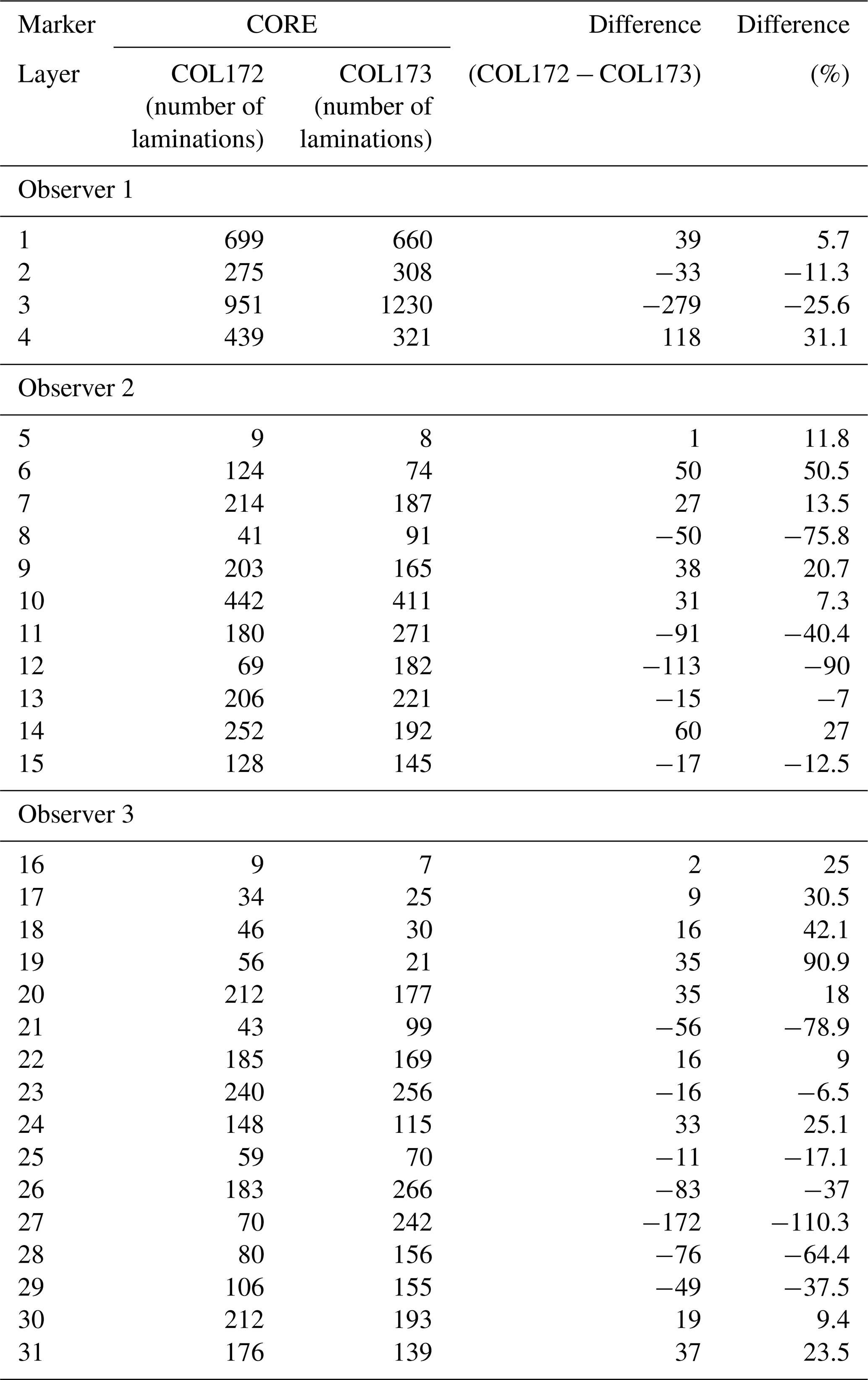
Table A2 Observer- and core-specific lamination statistics of thickness and counts. Lamination quality codes 4, 5, and 6 are excluded from the analysis except to calculate the cumulative length of indistinct sections. All units are millimeters unless otherwise noted.

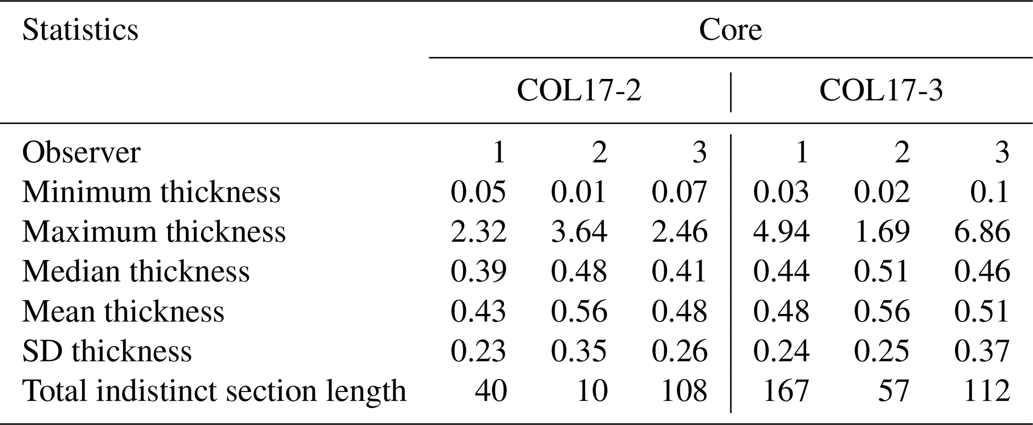
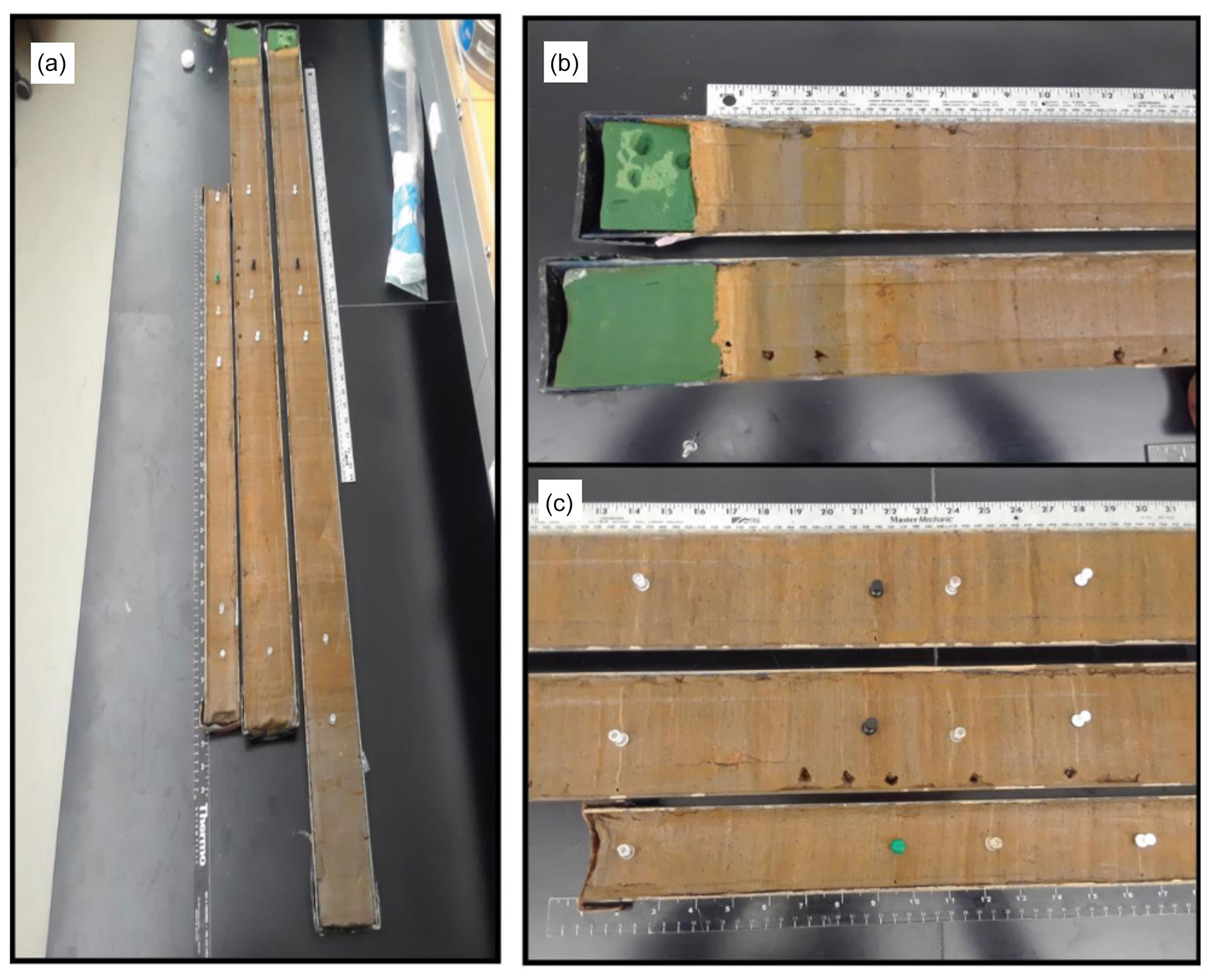
Figure A1 Tie points from three Columbine Lake cores. (a) COL17-2 on the far right, COL17-3 in the middle, and COL16-1 on the left. The top of cores COL-17-3 and COL17-2 are shown in (b). Panel (c) is a section of the middle of all three cores with matching laminations marked with pins. Image credit: C. Wiman (2019). Late Holocene hydroclimate and productivity in varved sediment at Columbine Lake, Colorado (Master thesis, Northern Arizona University).

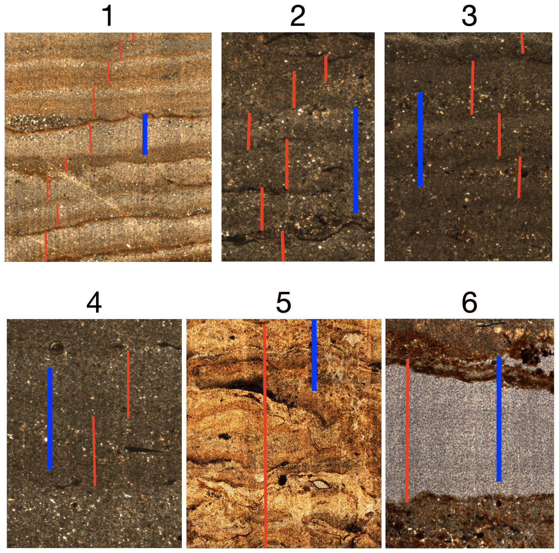
Figure A2 Examples of appearance for each lamination quality code for Columbine Lake sediment. The blue bar is 1 mm in all images.

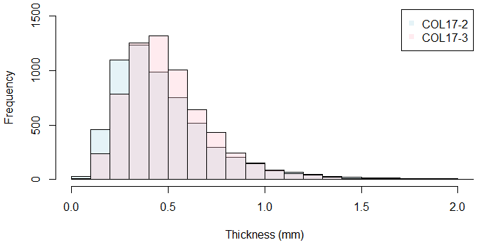
Figure A3 Comparison of lamination thickness measurements from sections with codes 1, 2, and 3 between COL17-2 and COL17-3. Blue represents COL17-2, red represents COL17-3, and the overlap of the two distributions is light purple.

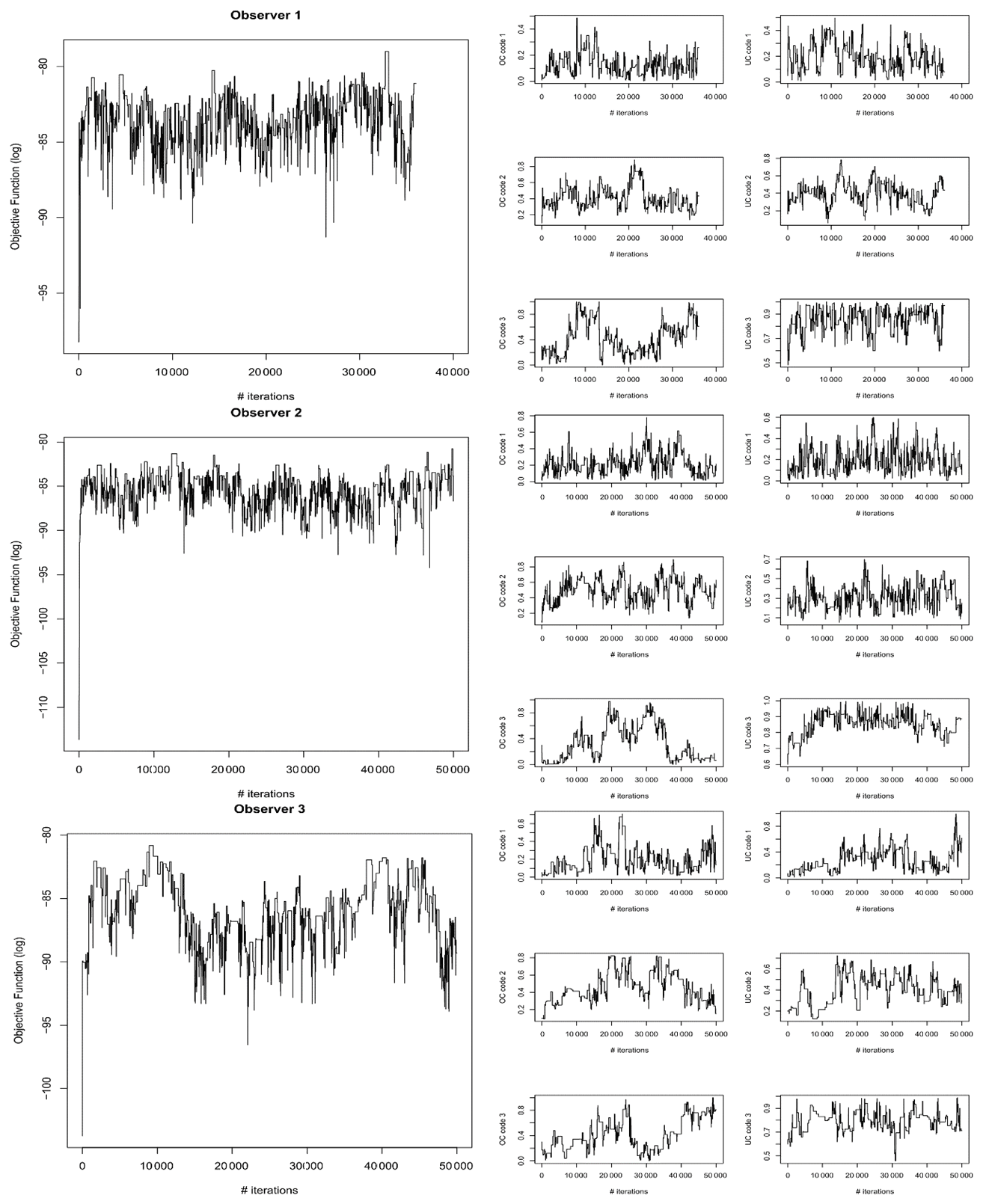
Figure A4 Integrated model diagnostics. Objective function output value (left) and counting probabilities (right) for each iteration for observers 1 (top), 2 (middle), and 3 (bottom). OC: over-counting. UC: under-counting. The number that follows OC and UC indicates the varve quality code.

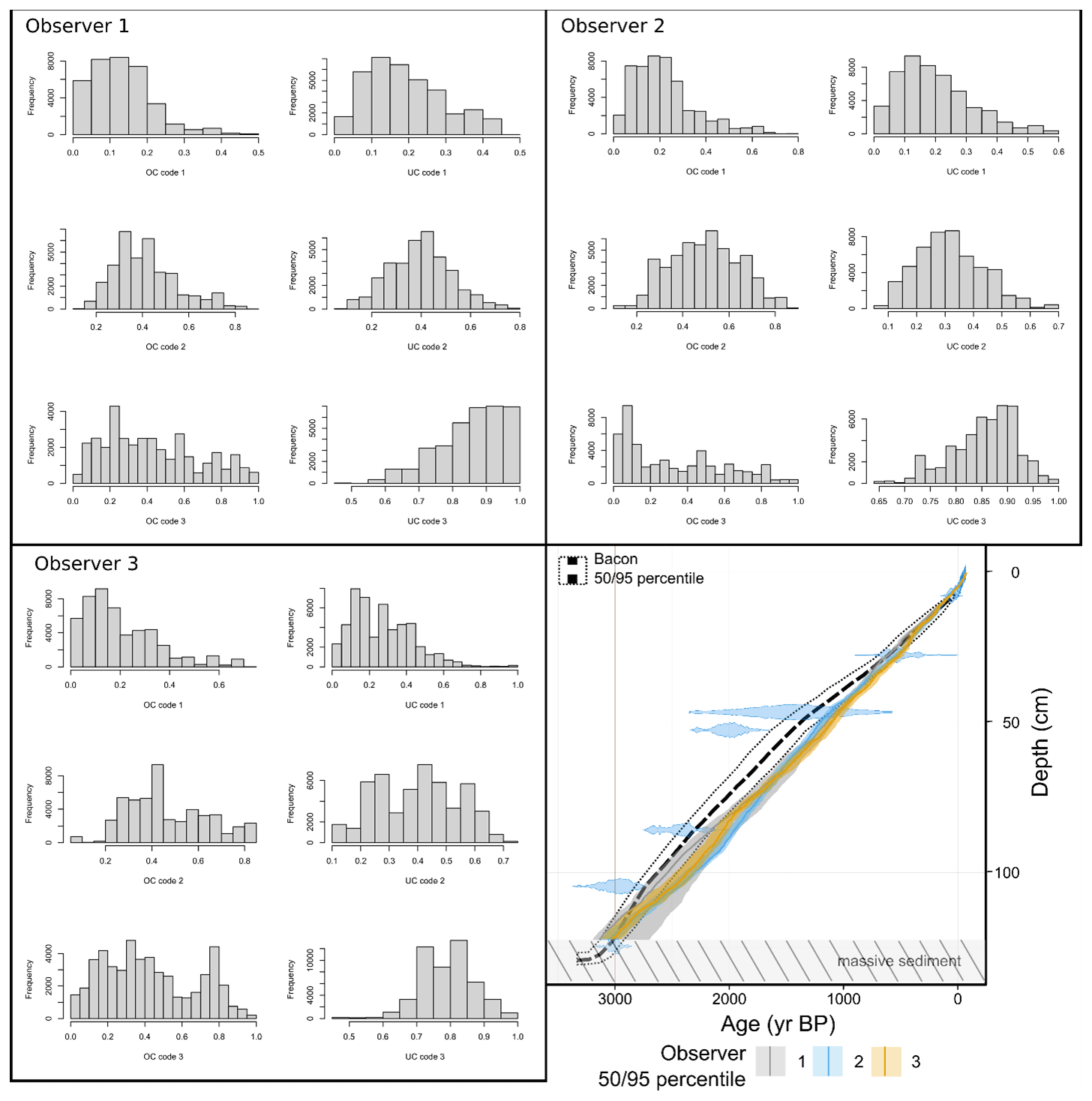
Figure A5 Posterior probabilities of over- and under-counting for each observer for core COL17-3. Comparison between independent and integrated age–depth model. OC: over-counting. UC: under-counting. Code 1–3 indicate the lamination quality codes 1–3.

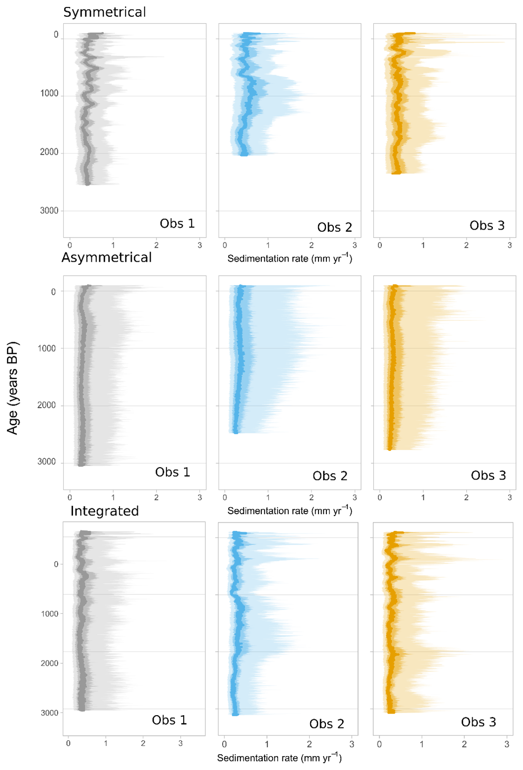
Figure A6 Sedimentation rates for each observer for the symmetrical varve-only model, asymmetrical varve-only model, and integrated models.