Combined linear-regression and Monte Carlo approach to modeling exposure age depth profiles

We introduce a set of methods for analyzing cosmogenic-nuclide depth profiles that formally integrates denudation and muogenic production, while retaining the advantages of linear inversion for surfaces with inheritance and age much greater than zero. For surfaces with denudation, we present solutions for both denudation rate and total denudation depth, each with their own advantages. By combining linear inversion with Monte Carlo simulation of error propagation, our method jointly assesses uncertainty arising from measurement error and denudation constraints. Using simulated depth profiles and natural-example depth profile data sets from the Beida River, northwest China, and Lees Ferry, Arizona, we show that our methods robustly produce accurate age and inheritance estimations for surfaces under varying circumstances. For surfaces with very low inheritance or age, it is important to apply a constrained inversion to obtain the correct result distributions. The denudation-depth approach can theoretically produce reasonably accurate age estimates even when total denudation reaches 5 times the nucleon attenuation length. The denudation-rate approach, on the other hand, has the advantage of allowing direct exploration of trade-offs between exposure age and denudation rate. Out of all the factors, lack of precise constraints for denudation rate or depth tends to be the largest contributor of age uncertainty, while negligible error results from our approximation of muogenic production using the denudation-depth approach.

1 Introduction

In situ terrestrial cosmogenic nuclide (CN) dating, especially with ¹⁰Be, is a widely applied tool to estimate landform ages (e.g., Granger et al., 2013). These dates are affected by landscape processes that either remove or add CNs, lending uncertainty that may be difficult to assess without additional information. Ages of landforms constructed from sediments, such as a stream terrace, may be affected by CNs acquired by the sediments prior to deposition, termed inheritance, leading to erroneously older dates (Brocard et al., 2003; Hancock et al., 1999; Repka et al., 1997). Conversely, even a low rate of denudation of a landform after its formation will bias surface-exposure ages younger (Lal, 1991). Under the condition of no denudation, solving a depth profile of CN concentrations via linear inversion – a technique first developed by Anderson et al. (1996) – provides a robust approach for estimating surface age and inheritance from a landform comprised of sediments. However, this method suffers from the deficit of not incorporating denudation or muogenic production process and has been succeeded by forward-modeling approaches (e.g., Hidy et al., 2010). Despite its deficits, however, linear regression retains advantages as a robust and straightforward approach to invert for exposure age. Herein we revisit the application of linear regression for CN depth profiles with an updated approach, building upon the simplicity of the original technique, but expanding its application to surfaces with independently constrained denudation histories, and increasing the accuracy of the age and inheritance results by taking muogenic production into account.

As an inverse approach, our least-squares linear regression directly solves for a best-fit age and inheritance, while treating the denudation rate or denudation depth as a model input, rather than an output of the model. It may be used with Monte Carlo sampling to explore the full distribution of possible ages and inheritance from the variation of input parameters. As an inverse approach, linear regression directly returns a best estimate, providing a clear way to explore how model inputs, such as erosion, affect the result. This is useful to derive an exposure age directly, or as a starting point for forward models (e.g., Hidy et al., 2010; Laloy et al., 2017; Marrero et al., 2016). In the latter case, linear inversion may help researchers tune the boundary values for the forward models to get better simulation results.

In this paper, we present a general inversion which incorporates muogenic production as a summation of exponential terms (e.g., Heisinger et al., 2002a, b), and two specific approaches for age inversion at sites with constant denudation rate. The first of these approaches applies a constant denudation rate but requires simplification by omitting muogenic production. This approach provides a useful tool to explore the trade-offs between denudation rate and exposure age but introduces systematic errors as denudation rate increases due to the exclusion of muogenic production. The second approach introduces a solution for a constant denudation depth with a Taylor-series approximation for the muogenic production terms. With this approximation, linear regression produces robust age estimates even for surfaces with a large amount of denudation. To show the application of these techniques, we present applications to pseudo-realistic depth profiles under various scenarios. We also apply our approach to two previously published example sample sites, one from the Beida River in western China from our own work (Wang et al., 2020) and one from the Lees Ferry site on the Colorado River from Hidy et al. (2010), to demonstrate model performance for realistic cases. These examples show that our revised linear-regression approach is robust and can be applied to most exposure dating scenarios.

2 Methods

2.1 General inversion

Under conditions of constant production rate and constant denudation rate, a surface that was exposed at time t would have a concentration of a cosmogenic nuclide (N_z) as follows (Balco et al., 2008; Braucher et al., 2009; Lal, 1991; Lal and Arnold, 1985):

$$\begin{array}{}\text{(1)}& \begin{array}{rl}{N}_z\left(t\right)& =P_{n,\mathrm{0}}{e}^{-\frac{\mathit{\rho }z}{{\mathrm{\Lambda }}_n}}\left({\displaystyle \frac{\mathrm{1}-e^{-\left(\frac{\mathit{\rho }\mathit{\epsilon }}{{\mathrm{\Lambda }}_n}+\mathit{\lambda }\right)t}}{\frac{\mathit{\rho }\mathit{\epsilon }}{{\mathrm{\Lambda }}_n}+\mathit{\lambda }}}\right)\\ & +P_{m_{\mathrm{1}},\mathrm{0}}{e}^{-\frac{\mathit{\rho }z}{{\mathrm{\Lambda }}_{m_{\mathrm{1}}}}}\left({\displaystyle \frac{\mathrm{1}-e^{-\left(\frac{\mathit{\rho }\mathit{\epsilon }}{{\mathrm{\Lambda }}_{m_{\mathrm{1}}}}+\mathit{\lambda }\right)t}}{\frac{\mathit{\rho }\mathit{\epsilon }}{{\mathrm{\Lambda }}_{m_{\mathrm{1}}}}+\mathit{\lambda }}}\right)\\ & +P_{m_{\mathrm{2}},\mathrm{0}}{e}^{-\frac{\mathit{\rho }z}{{\mathrm{\Lambda }}_{m_{\mathrm{2}}}}}\left({\displaystyle \frac{\mathrm{1}-e^{-\left(\frac{\mathit{\rho }\mathit{\epsilon }}{{\mathrm{\Lambda }}_{m_{\mathrm{2}}}}+\mathit{\lambda }\right)t}}{\frac{\mathit{\rho }\mathit{\epsilon }}{{\mathrm{\Lambda }}_{m_{\mathrm{2}}}}+\mathit{\lambda }}}\right),\end{array}\end{array}$$

where P_n,0, $P_{m_{\mathrm{1}},\mathrm{0}}$, and $P_{m_{\mathrm{2}},\mathrm{0}}$ are the surface production rate induced by nucleons, negative muons, and fast muons, and Λ_n, ${\mathrm{\Lambda }}_{m_{\mathrm{1}}}$, and ${\mathrm{\Lambda }}_{m_{\mathrm{2}}}$ are the attenuation scale lengths (g cm⁻²) of the nucleons and muons (negative and fast), respectively. Note that the two exponential terms for muogenic production used here are an approximation of a complex muogenic production path, because the muon energy spectrum hardens continuously with depth (Heisinger et al., 2002a, b; Marrero et al., 2016; Balco, 2017). z is the depth beneath the target surface; λ is the decay constant, and ε is a constant denudation rate, if applicable. For our purposes, we model ages using ¹⁰Be, with a half-life of 1.39 Myr (Chmeleff et al., 2010; Korschinek et al., 2010), due to its wide applicability to quartz-bearing sediments (Cockburn and Summerfield, 2004; Granger et al., 2013; Rixhon et al., 2017).

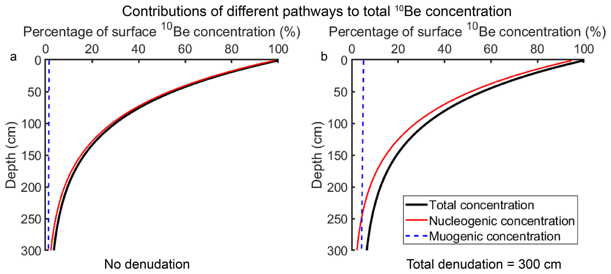
Figure 1 Depth–concentration profiles with different contributing components for a hypothetical surface. The profiles are calculated based on a sea level high-latitude production rate (nucleogenic production rate of 4.11 atoms g⁻¹, Martin et al., 2017; muogenic production rate of 0.0735 atoms g⁻¹, Balco, 2017). All the concentrations are normalized to a percentage of the total surface concentration. (a) Surface with no denudation. (b) Surface with steady denudation rate; denudation depth equal to 300 cm.

Based on Eq. (1), the production of cosmogenic nuclides may be simplified into two major components: the production rate at specific depth (P_z) and the effective exposure age of the site (T_e), which is the time that is required to accumulate concentration N_z at production rate P_z without erosion and radioactive decay. Therefore Eq. (1) may be rearranged into

$$\begin{array}{}\text{(2a)}& N_z\left(t\right)=\sum _i{P}_{zi}{T}_{ei},\end{array}$$

where

$$\begin{array}{}\text{(2b)}& \begin{array}{rl}& P_{zi}=P_{i,\mathrm{0}}{e}^{-\frac{\mathit{\rho }z}{{\mathrm{\Lambda }}_i}}{T}_{ei}=\left({\displaystyle \frac{\mathrm{1}-e^{-\left(\frac{\mathit{\rho }\mathit{\epsilon }}{{\mathrm{\Lambda }}_i}+\mathit{\lambda }\right)t}}{\frac{\mathit{\rho }\mathit{\epsilon }}{{\mathrm{\Lambda }}_i}+\mathit{\lambda }}}\right),\\ & i=n,m_{\mathrm{1}},m_{\mathrm{2}}.\end{array}\end{array}$$

The ¹⁰Be concentration measured from a suite of samples (Fig. 1), C, has two components: the in situ produced concentration, N_z, and the inherited concentration, C_inh,

$$\begin{array}{}\text{(3)}& C=\sum _i{P}_{zi}{T}_{ei}+C_{\mathrm{inh}}.\end{array}$$

However, ¹⁰Be concentration (C) is exponential to the burial depth, based on Eqs. (2) and (3), when there is no denudation ($\mathit{\epsilon }\approx \mathrm{0})T_{en}=T_{e{m}_{\mathrm{1}}}=T_{e{m}_{\mathrm{2}}}$, and therefore Eq. (3) can be rearranged as follows:

$$\begin{array}{}\text{(4a)}& C=T_e\sum _i{P}_{zi}+C_{\mathrm{inh}},\end{array}$$

where

$$\begin{array}{}\text{(4b)}& T_e=\left({\displaystyle \frac{\mathrm{1}-e^{-\mathit{\lambda }t}}{\mathit{\lambda }}}\right).\end{array}$$

This equation is an update to the linear-regression approach first proposed by Anderson et al. (1996) that accounts for both nucleon and muon production, as well as radioactive decay. For the case of no denudation, CN concentration is linear to the sum of production rates via all pathways $\left(\sum _i{P}_{zi}\right)$, and T_e and C_inh are the slope and intercept of this linear relationship, respectively. Therefore, similar to the approach proposed by Anderson et al. (1996), we can apply least-squares linear regression to find the slope (T_e) and intercept (C_inh) of the best-fit line to the concentration vs. production rate data of the depth profile. The exposure age, factoring in decay, may be calculated directly by rearranging Eq. (4b):

$$\begin{array}{}\text{(5)}& t=-{\displaystyle \frac{\ln \left(\mathrm{1}-T_e\mathit{\lambda }\right)}{\mathit{\lambda }}}.\end{array}$$

2.2 Inversion with denudation rate

For sites with constant denudation rate, ε, the effective age for each pathway (nucleons or muons) would be different, due to their different attenuation lengths. But an approximation may be made by omitting the muogenic production, on the basis that muogenic production only makes up a very small fraction of the total surface production (Braucher et al., 2003, 2011, 2013; Heisinger et al., 2002b, a; Balco et al., 2008; Balco, 2017), and Eq. (3) may be further simplified to

$$\begin{array}{}\text{(6)}& C=P_{zn}{T}_{en}+C_{\mathrm{inh}}.\end{array}$$

Using Eq. (6), a linear least-squares regression can be applied to find the best-fit T_en and C_inh, which leads to the estimated exposure age

$$\begin{array}{}\text{(7a)}& t=-{\displaystyle \frac{\ln \left(\mathrm{1}-T_{en}B\right)}{B}},\end{array}$$

where

$$\begin{array}{}\text{(7b)}& B={\displaystyle \frac{\mathit{\rho }\mathit{\epsilon }}{{\mathrm{\Lambda }}_n}}+\mathit{\lambda }.\end{array}$$

This solution illustrates the utility of separating the age model for finding T_en from the effect of denudation rate, contained within the parameter B. Though the error introduced to omitting muogenic production grows as the denudation rate increases, this approach (Eq. 7) provides a useful tool to examine the relationship between exposure age and denudation rate.

2.3 Inversion with denudation depth

For many practical cases, it may be more straightforward to estimate total denudation depth (D) from field evidence such as through soil-profile analysis, rather than a denudation rate (e.g., Ebert et al., 2012; Hidy et al., 2010; Ruszkiczay-Rüdiger et al., 2016). With denudation depth, the effective age of each pathway may be rewritten as

$$\begin{array}{}\text{(8)}& T_{ei}=\left({\displaystyle \frac{\mathrm{1}-e^{-\left(\frac{\mathit{\rho }D}{{\mathrm{\Lambda }}_i}+\mathit{\lambda }t\right)}}{\frac{\mathit{\rho }D}{{\mathrm{\Lambda }}_{i}t}+\mathit{\lambda }}}\right),i=n,m_{\mathrm{1}},m_{\mathrm{2}}.\end{array}$$

Here we explore the application of this equation with the inclusion of muogenic production. Using a series expansion, we rewrite the effective age related to muons (negative and fast), T_em, into a fraction, g, of the effective age related to nucleons, T_en. The fraction g can be approximated solely from knowledge of the denudation depth, D (see Appendix for derivation):

$$\begin{array}{}\text{(9)}& \begin{array}{rl}& g_i={\displaystyle \frac{T_{emi}}{T_{en}}}\approx e^{-\frac{\mathrm{1}}{\mathrm{2}}\left(\frac{\mathit{\rho }D}{{\mathrm{\Lambda }}_{mi}}-\frac{\mathit{\rho }D}{{\mathrm{\Lambda }}_n}\right)+\frac{\mathrm{1}}{\mathrm{24}}\left[{\left(\frac{\mathit{\rho }D}{{\mathrm{\Lambda }}_{mi}}\right)}^{\mathrm{2}}-{\left(\frac{\mathit{\rho }D}{{\mathrm{\Lambda }}_n}\right)}^{\mathrm{2}}\right]},\\ & i=\mathrm{1},\mathrm{2}.\end{array}\end{array}$$

Bringing g_i into Eq. (3), we have

$$\begin{array}{}\text{(10)}& \begin{array}{rl}C\left(z\right)& =P_{zn}{T}_{en}+P_{z{m}_{\mathrm{1}}}{g}_{\mathrm{1}}{T}_{en}+P_{z{m}_{\mathrm{2}}}{g}_{\mathrm{2}}{T}_{en}+C_{\mathrm{inh}}\\ & =P_{ze}{T}_{en}+C_{\mathrm{inh}},\\ P_{ze}& =\left(P_{zn}+P_{z{m}_{\mathrm{1}}}{g}_{\mathrm{1}}+P_{z{m}_{\mathrm{2}}}{g}_{\mathrm{2}}\right),\end{array}\end{array}$$

where P_ze is the effective production rate from both nucleons and muons under the condition of a finite amount of steady denudation over the lifetime of the deposit.

Using Eq. (10), T_en and C_inh can be found by applying least-squares linear regression with known production rates, denudation, and sample concentrations, similar to the general inversion case for no denudation described by Eq. (4).

To estimate the exposure age, we need to find the solution for

$$\begin{array}{}\text{(11)}& f\left(t\right)=\left({\displaystyle \frac{\mathrm{1}-e^{-\left(\frac{\mathit{\rho }D}{t{\mathrm{\Lambda }}_n}+\mathit{\lambda }\right)t}}{\frac{\mathit{\rho }D}{t{\mathrm{\Lambda }}_n}+\mathit{\lambda }}}\right)-T_{en}=\mathrm{0}.\end{array}$$

While the complicated form of Eq. (11) prohibits a direct solution, t may be found iteratively by applying the Newton's method. Using the derivative of Eq. (11),

$$\begin{array}{}\text{(12)}& f^{\prime }\left(t\right)=-\mathit{\lambda }{e}^{-\left(\frac{\mathit{\rho }D}{{\mathrm{\Lambda }}_n}\right)D-\mathit{\lambda }t}-{\displaystyle \frac{\mathit{\rho }D{T}_{en}}{{\mathrm{\Lambda }}_n{t}^{\mathrm{2}}}},\end{array}$$

the exposure age can then be iterated from

$$\begin{array}{}\text{(13)}& t_{n+\mathrm{1}}=t_n-{\displaystyle \frac{f\left(t_n\right)}{f^{\prime }\left(t_n\right)}}\end{array}$$

with initial guess, t₀=T_en.

3 Applications

We present a set of example applications of linear regression to CN depth profiles using both the denudation-rate (Eqs. 6, 7) and the denudation-depth (Eqs. 8–13) techniques. We begin with simulated CN depth profiles to explore the impacts of scatter of sample concentration, low inheritance, denudation, and sample depth on the accuracy and precision of our approach, and to compare the performance of linear regression with the estimations using a Monte Carlo Markov chain approach. We then demonstrate the linear-regression technique with two case examples. For the Beida River T2 terrace of the North Qilian Shan, China (Wang et al., 2020), we demonstrate using the denudation-rate approach to explore the possible range of exposure age and the trade-offs between age and denudation rate; we also demonstrate how to use the denudation-depth approach combined with Monte Carlo simulation to estimate the full distribution of exposure age and inheritance. For the Lees Ferry site on the Colorado River (Hidy et al., 2010), we compare results from our denudation-depth approach with the original publication.

To explore the full distribution of possible estimated age and inheritance, we consider the uncertainty propagated from five different sources: uncertainty of the ¹⁰Be concentration measurements, uncertainty of sample depths, uncertainty of sediment density, uncertainty of the denudation depth or rate, and the uncertainties related to CN production and decay (i.e., the attenuation lengths, production rates, etc.). These uncertainties propagate sequentially, first from ¹⁰Be concentration, sample depths, and sediment density through the least-squares linear-regression process, and second from denudation rate or depth through converting exposure age from the effective exposure age (T_e). Because of the limited sample sizes typical of most studies, and the variance in both concentration and depth, we apply a Monte Carlo sampling approach for the range of each input parameter. The code used here is archived in GitHub (https://github.com/YiranWangYR/10BeLeastSquares, last access: 15 August 2022; Wang, 2022). Our procedure includes the following steps.

• Step 1: generate all the input parameters for one model – sampling distributions for ¹⁰Be concentration, sample depth, density, denudation rate or depth, production rate, attenuation length, etc. Depending on the parameter, we represent uncertainty as either a normal or uniform distribution.

• Step 2: fit these sampled input parameters with Eq. (4) or Eq. (6) or Eq. (10) to derive best-fit sample T_en and inheritance values.

• Step 3: calculate the exposure age use T_en from step 2 and parameters generated from step 1 using Eq. (5) or Eq. (7) or Eqs. (11)–(13).

• Repeat steps 1–3 for many times to produce a distribution of age and inheritance results.

3.1 Simulated CN depth profiles

To demonstrate how our approach will perform under different circumstances, we generate a series of simulated depth profiles to test how closely the estimated age and inheritance will reflect the true values. With these profiles, four different scenarios are tested: varying degrees of random deviation of sample concentrations, varying amount of denudation, low inheritance, and deep sample depth. For comparison, we use a forward model which operates with a Monte Carlo Markov chain algorithm (codes: https://github.com/YiranWangYR/10BeLeastSquares/blob/main/Be10_LRvsBayesian.m, last access: 15 August 2022; Wang, 2022) to estimate the exposure age and inheritance along with our linear-regression approach. We choose to use our own coding following Bayesian inversion principles instead of published codes because, first, we need to ensure the input variables are the same for both approaches, and second, to be statistically significant, we need to apply both approaches several hundred times for each scenario; therefore manually doing so with published codes would be extremely time consuming.

Table 1 Parameters used for each simulation scenario.

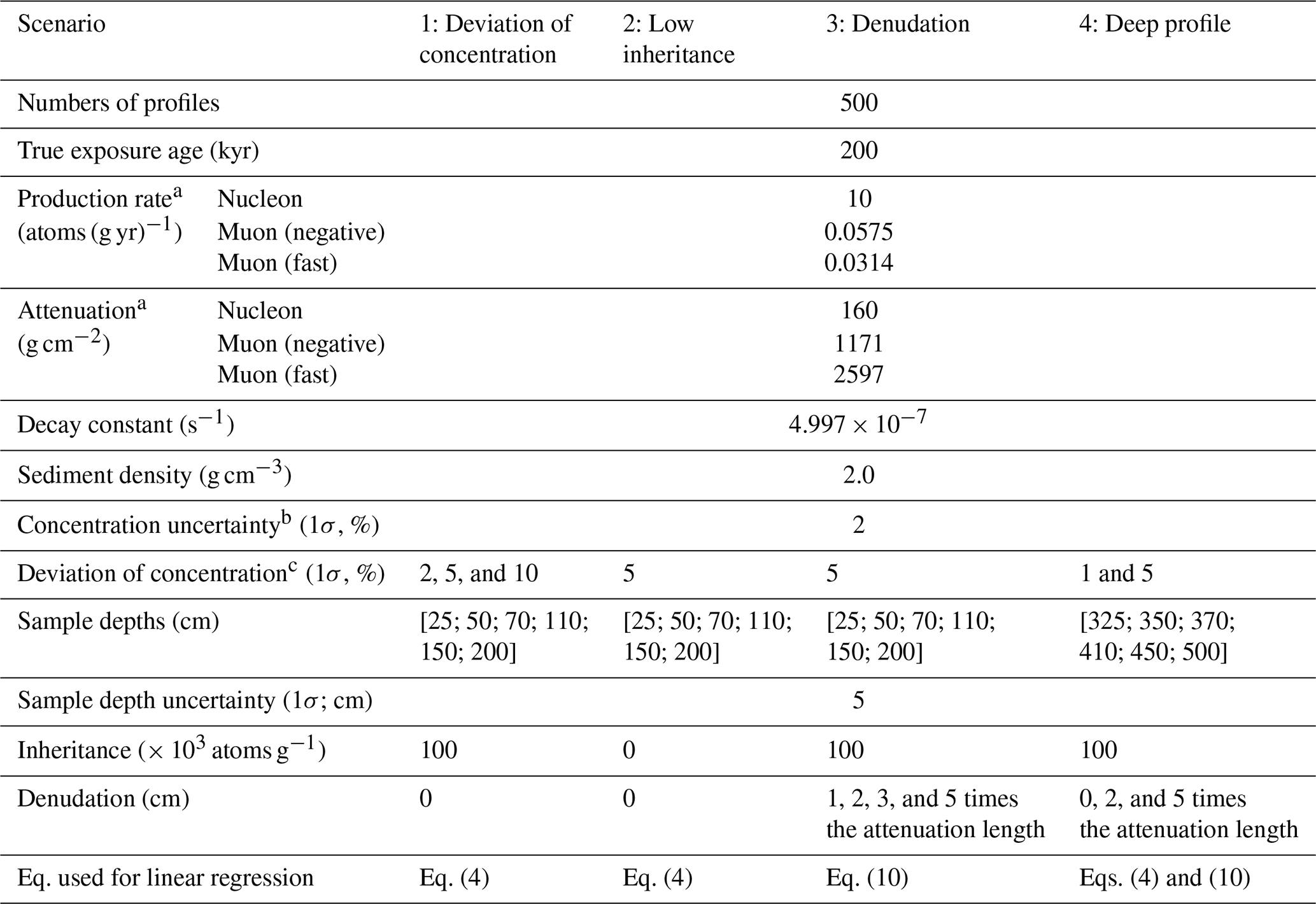
^a Production rate and attenuation length are calculated (nucleon) and approximated (muon) based on a hypothetical middle-latitude, 1000 m elevation site (Stone, 2000; Balco, 2017). ^b The analytical uncertainty of sample concentration. ^c The amount that the mean sample concentration deviates from the true concentration.

For all simulated profiles, we set the true age and inheritance to be 200 kyr and 100 × 10³ atoms g⁻¹ except for the low-inheritance scenario, where we set inheritance to 0 and 5000 atoms g⁻¹. Each simulated profile contains six samples; to mimic realistic scatter of sample concentrations, all the simulated samples are deviated from the true profile based on an assigned normal distribution of either 1 %, 2 %, 5 %, or 10 % standard deviation. Analytical uncertainties (2 % standard deviation) are assigned to each sample of the simulated profile to mimic realistic values. For each scenario, 500 simulated profiles are generated and inverted for age and inheritance using both the linear-regression and forward approaches. The details of our simulation process and the parameters we used for each scenario are listed in Table 1.

3.1.1 Deviation of sample concentrations

We test three sets of simulations under different degrees of imposed deviation of sample concentrations (standard deviation of 2 %, 5 %, and 10 %) with no denudation. The 2 % deviation case matches the analytical uncertainty (2 %), while the 5 % and 10 % cases introduce excess scatter, as is typically found in CN depth profiles. For the case with 2 % of deviation, we find both linear-regression and forward approaches yield results centered around the true age (200 kyr). For the linear-regression approach, 95 % of the mean ages fall within 4.0 %–4.5 % error range of the true age, while for the forward approach 95 % of the mean age fall within 3.0 %–3.5 % error range of the true age. The forward approach works slightly better than linear regression for the more extreme (noisier) cases (Fig. 2 and Fig. S1 in the Supplement). For inheritance estimation, similar to the exposure age, both approaches return results centered around the true value (100 000 atoms g⁻¹), and a forward approach again performs somewhat better for noisier data. When the sample deviation increases to 5 %, then to 10 %, the estimated age and inheritance values remain centered on the correct age and inheritance while the ranges of the mean estimations for both approaches expand significantly, indicating a decrease in precision as the noise level increases (Figs. 2, S1–S3). With 5 % of deviation, 95 % of the estimated ages fall within 10 % and 8 % ranges of the true value for linear-regression and forward approach, respectively. With 10 % of deviation, 95 % of the estimated age fall within 21 % and 17 % ranges of the true value for linear-regression and forward approach, respectively. We also find the error range for the estimation results from the linear regression is moderately larger than a forward approach (Figs. S1–S3). Importantly, we find that while each approach provides different estimation results for the same set of samples, one model does not consistently perform better than the other (Figs. S1–S3). About 40 %–45 % of the time the linear regression returns results closer to the true age than the forward approach.

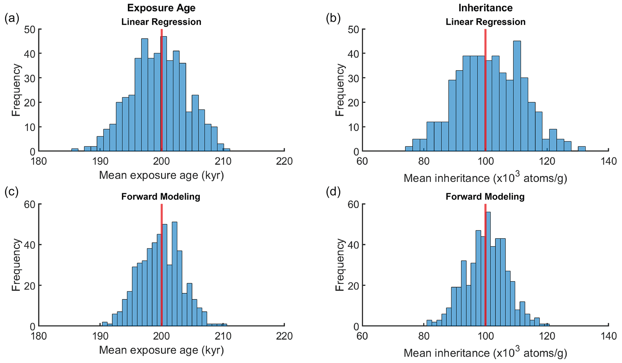
Figure 2 Distribution of mean exposure age (a, c) and inheritance (b, d) estimated from linear-regression (Eq. 4; a, b) and a forward approach (c, d) for 500 simulated profiles with 2 % of imposed sample deviation. Red vertical line annotates the true age and true inheritance.

3.1.2 Low inheritance or exposure age

One important constraint for our inversion (Eqs. 6 and 10) is that both inheritance (C_inh) and the effective exposure age (T_en) should not be negative. This constraint is not important when both C_inh and T_en are much greater than zero, as none of the inverted results will fall below zero. However, when either one of these variables is small enough, inverting without a positivity constraint may lead to incorrect uncertainty distributions. We demonstrate this by using profiles generated with 5 % imposed deviation of sample concentrations and zero inheritance (Table 1). Here we compare three different scenarios: (1) not permitting negative inheritance during inversion through setting the boundary condition, C_inh≥0; (2) permitting negative inheritance during inversion; and (3) excluding negative inheritance outcomes after inversion. Notice that scenario 1 is a constrained inversion (nonnegative least square problem; solution in Lawson and Hanson, 1987) while scenarios 2 and 3 are not constrained. The distributions of the mean exposure age and inheritance (Fig. 3) show that, in the first scenario, the positivity constraint forces all the possible negative inheritance to be exactly zero, which leads to an age distribution skewed to the left while still centering the true age (Fig. 3a, d). In the unconstrained scenarios (2), the uncertainty distribution for inheritance incorrectly extends to negative values, though the age results were distributed normally around the true age (Fig. 3b, e). When negative inheritance results are excluded after applying the unconstrained inversion (scenario 3), the inheritance results exhibit a clipped normal distribution, while the age is not only left-skewed but also shows obvious underestimation (Fig. 3c, f), resulting from discarding the older age estimations that were related to negative inheritance. Similarly, when inverting for a surface that is sufficiently young, or the inheritance is large relative to the surface age, the unconstrained regression could also lead to an age distribution extending to negative values.

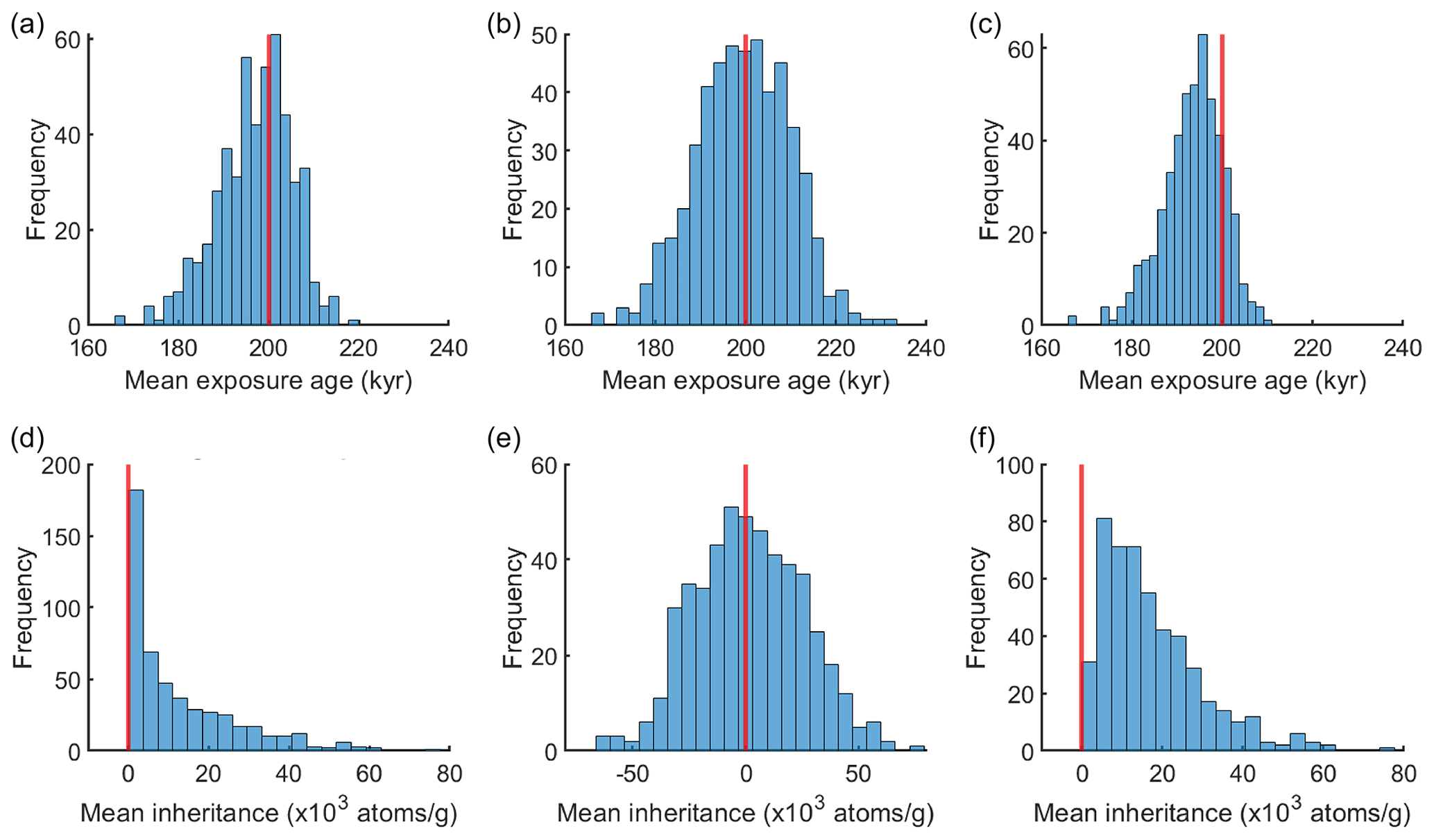
Figure 3 Distribution of mean exposure age (a–c) and inheritance (d–f) estimated from linear regression (Eq. 4) for 500 simulated profiles with 0 inheritance and 5 % of imposed sample deviation. (a, d) Not permitting negative inheritance during inversion. (b, e) Permitting negative inheritance during inversion. (c, f) Excluding negative inheritance results after inversion. Red vertical line annotates the true age and true inheritance.

3.1.3 Denudation depth

To test the robustness of our denudation-depth approach, we tested simulated CN depth profiles with total denudation of 1, 2, 3, and 5 times the nucleon-spallation attenuation length $\left(\frac{\mathit{\rho }}{{\mathrm{\Lambda }}_n}\right)$ and 5 % of imposed sample deviation (Table 1). The resulting distributions of the mean age (Fig. 4) are all well centered around the true age even with the largest amount of denudation tested. We also observe that when total denudation reaches 3 and 5 times the attenuation length, the ranges of the estimated mean age grow slightly wider, indicating a decrease in precision. This phenomenon can also be observed with the forward approach (Fig. S4), which suggests it is not a result of the approximation introduced through Eq. (9). Instead, we suggest this problem relates to a low concentration gradient for profiles with a large amount of denudation, making the inversion more sensitive to measurement error. We find that the distribution of the mean inheritance remains well centered around the true inheritance for all simulated profiles, even for profiles with denudation equal to 5 times the attenuation length.

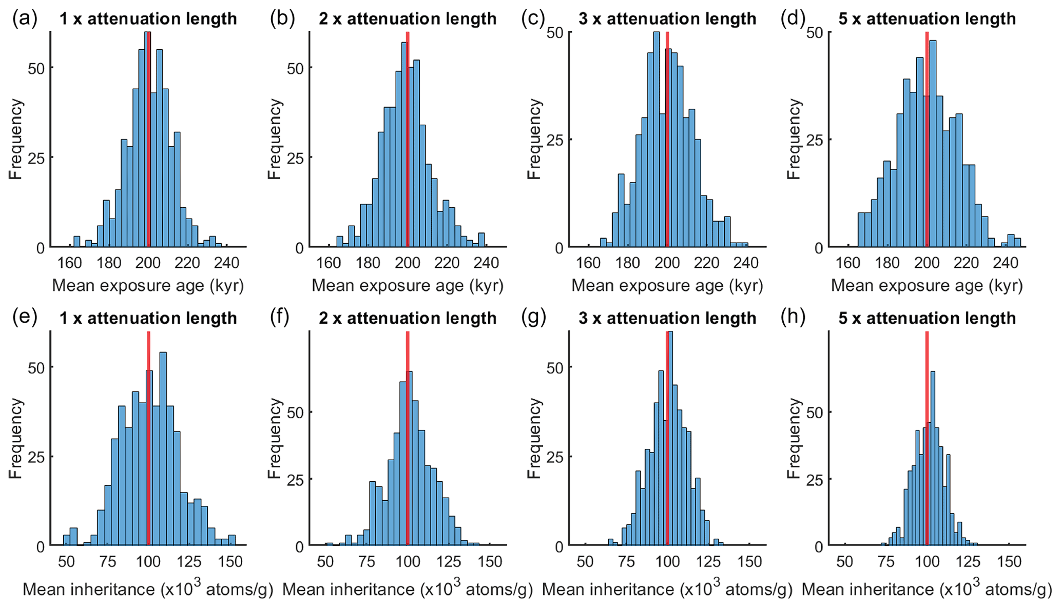
Figure 4 Distribution of mean exposure age (a–d) and inheritance (e–h) estimated from linear regression (Eq. 10) for 500 simulated CN profiles with 5 % of imposed sample deviation and with total denudation equals to 1 (a, e), 2 (b, f), 3 (c, g), and 5 times (d, h) the attenuation length of spallation. Red vertical line annotates the true age and true inheritance.

3.1.4 Deep sample profiles

Samples at depths greater than ∼ 2 m are especially sensitive to muogenic production (Fig. 1). Here we test our denudation-depth approximation with depth profile samples distributed between 3 and 5 m depth to mimic the situation when near surface samples are not obtainable. Three groups of profiles, subjected to a total denudation of 0, 2, and 5 times the spallation attenuation length and with 5 % of imposed sample deviation, are tested with both linear-regression and forward approach (Table 1).

Figure 5 Distribution of age estimations from linear-regression (a–c) and a forward approach (d–f) for 500 simulated CN deep (3–5 m) profiles with denudations equal to 0 (a, d), 2 (b, e), and 5 times (c, f) the attenuation length, and with 5 % imposed deviation of sample concentration.

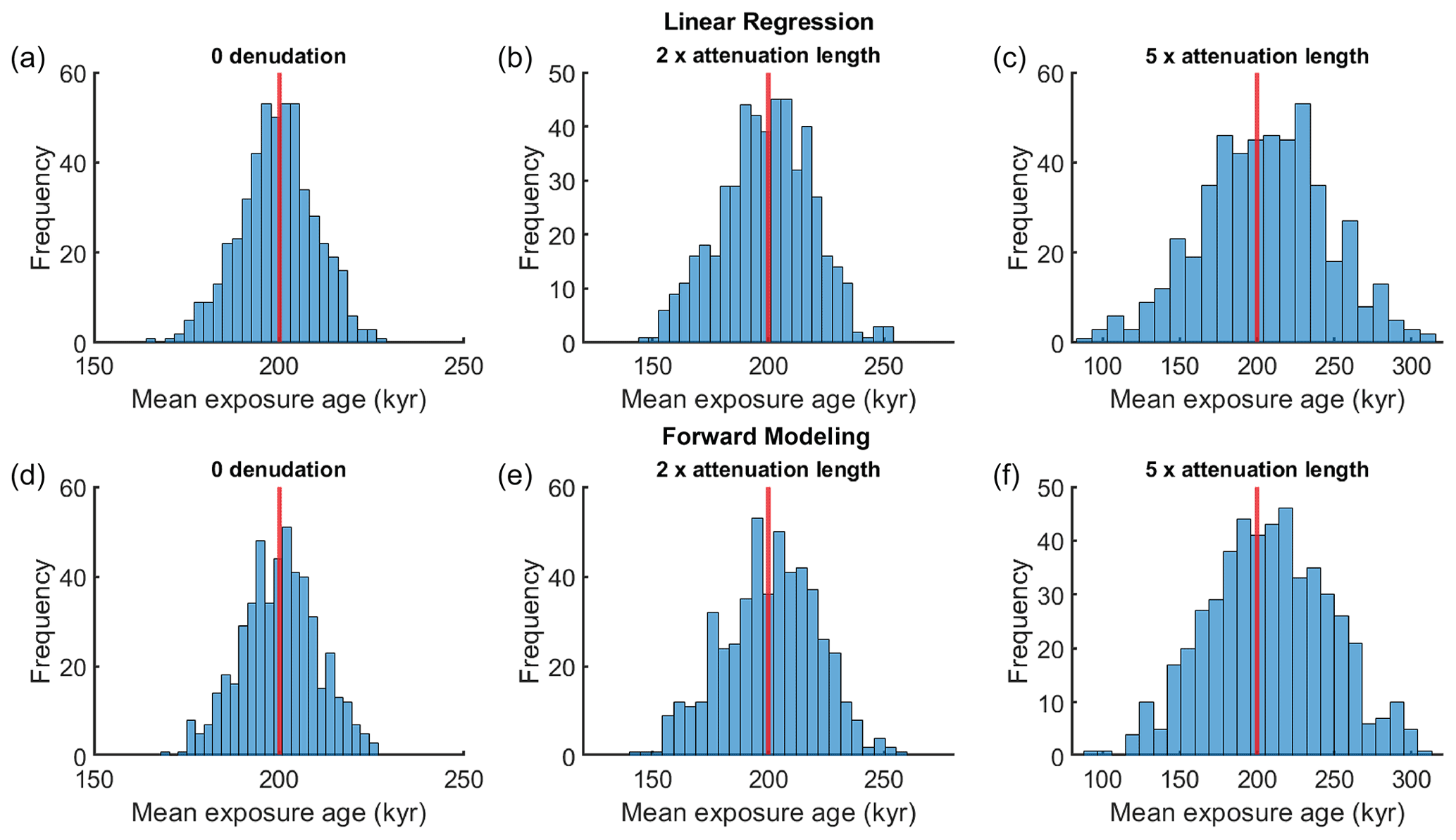
Figure 6 Distribution of age estimations from linear-regression (a–c) and a forward approach (d–f) for 500 simulated CN deep (3–5 m) profiles with denudations equal to 0 (a, d), 2 (b, e), and 5 times (c, f) the attenuation length, and with 1 % imposed deviation of sample concentration.

We find that compared to the near-surface profiles, results from the deep profiles show greatly reduced precision, especially for large denudation depths (Figs. 5, S5). The majority (95 % confidence) of the mean exposure ages estimated with linear regression spread between 100–300, 20–400, and 0–570 kyr, for surfaces with 0, 2, and 5 times the attenuation length of denudation, respectively (Fig. 5). This occurs with both linear-regression and forward approaches, indicating the precision drop is not due to our approximation of muogenic production (Eq. 9). Similar to the examples with large denudation (Fig. 4), we suggest the low precision is a result of the very low concentration gradient at depth. Different from near-surface profiles, a small change in the concentration gradient at depth leads to a large change of the estimated exposure age, which makes the inversion overly sensitive to random scatter of sample concentrations. As a comparison, by setting the imposed sample deviation to 1 % instead of 5 %, we find that precision increases greatly (Fig. 6). With linear regression, the majority (95 % confidence) of the mean exposure ages are distributed between 180–220, 162–242, and 131–275 kyr for 0, 2, and 5 times the attenuation length denudation, respectively (Figs. 6, S6). Thus, theoretically, both linear-regression and forward approach can produce accurate estimates if the scatter of sample concentrations is low. Reducing analytical uncertainty through use of large sample masses would be crucial for the success of a deep sample profile.

3.2 Case examples

Here we present two case examples to show the application of our linear-regression model to natural conditions. Wang et al. (2020) excavated a sample pit ∼ 2 m deep beneath the tread of a terrace deposit from the Beida River, within the North Qilian Shan, western China. The site is covered with 125 cm loess which was deposited continuously since 8.3 kyr. Beneath the loess cover, erosional truncation of the A and uppermost B horizon of the soil profile indicates that there may have been 20–60 cm of erosion of the terrace tread prior to the onset of loess accumulation. We collected six samples of medium to coarse sand from up to 2 m below the base of the loess. ¹⁰Be concentrations for these samples, corrected for loess accumulation using the approach of Hetzel et al. (2004) are listed in Table S1.

To explore the effect of denudation rate, we use the most likely concentrations for each sample and invert for a preliminary T_en and inheritance values of 99.3 kyr and 8.3 × 10³ atoms g⁻¹ respectively, using Eq. (6). Using Eq. (7), we generate a plot of exposure age vs. denudation rate based on the preliminary T_en value. The plot (Fig. 7) shows that if there has been no denudation, the sample site has a minimum exposure age of ∼ 102 kyr prior to loess accumulation. This exposure age increases to 160 and 240 kyr when the denudation equals to 1 and 2 times the attenuation length, respectively. When the denudation rate reaches ∼ 0.7 cm kyr⁻¹, the CN accumulation and denudation reach equilibrium and no age may be determined.

Figure 7 Exposure age–denudation rate relationship of the Beida River terrace.

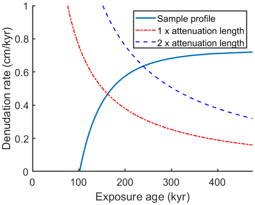
Figure 8 Linear-regression results for Beida River T2 terrace using the denudation-depth approach after 100 000 iterations. (a) Relationship of sample concentration to production rate at depth. Grey lines are the best-fit lines through this data set; (b) distribution of depth profile models with best-fit curves (grey lines). (c) Distribution of the effective exposure age (T_e); (d) distribution of the inherited ¹⁰Be concentration prior to loess accumulation. (e) Distribution of exposure age estimates derived from T_en values from linear regression (c). (f) Distribution of denudation rates predicted by the model; (g) distribution of sampled total denudation depth. Red lines indicate 95 % confidence range, green line indicates the median of the distribution, blue line indicates the mean of the distribution.

To explore the full distribution of potential age and inheritance results, we apply a Monte Carlo sampling of the sample concentrations, depths, denudation depth, etc. (Table S2). Using a normal distribution for the denudation depth with 40 cm as the mean and 10 cm as the standard deviation, we apply least-squares linear inversion with Eq. (10). Best-fit results for ¹⁰Be concentration (C₁) and effective production rate (P_ze) are shown in Fig. 8a, and the corresponding fitted depth profile curves are shown in Fig. 8b. With positivity constraints enforced, the inverted T_en and inheritance values are 86.3–107.2 kyr and 0–6.4 × 10⁴ atoms g⁻¹, respectively (ranges correspond to the 95 % confidence distributions for each value, Fig. 8c and d). The corresponding exposure age, calculated following Eqs. (11)–(13), is 108.6–150.6 kyr (2σ) prior to loess accumulation (Fig. 8e). The corresponding erosion rate is 0.18–0.42 cm kyr⁻¹ (Fig. 8f and g). Without positivity constraints for the inheritance, the resulting exposure age and inheritance would be 108.8–155.0 kyr and −4.7 × 10⁴ to +6.4 × 10⁴ atoms g⁻¹ (2σ) instead.

Hidy et al. (2010) reported a ¹⁰Be depth profile from the Lees Ferry site, excavated on top of a Colorado River fill terrace. Based on the soil profile, a total erosion of 0–30 cm is estimated for the sample site. For this site Hidy et al. (2010) applied their Monte Carlo model and originally reported an exposure age and inheritance of 69.8–103 kyr, and 6.97–10.70 atoms g⁻¹, respectively (95 % confidence). After updates of their code (v1.2, Hidy et al., 2010; Mercader et al., 2012), including the incorporation of a Bayesian fitting process, their model provides a new age estimation of 76.6–96.1 kyr. See Hidy et al. (2010) for more details of the sample site, sampling and processing, and age result interpretation.

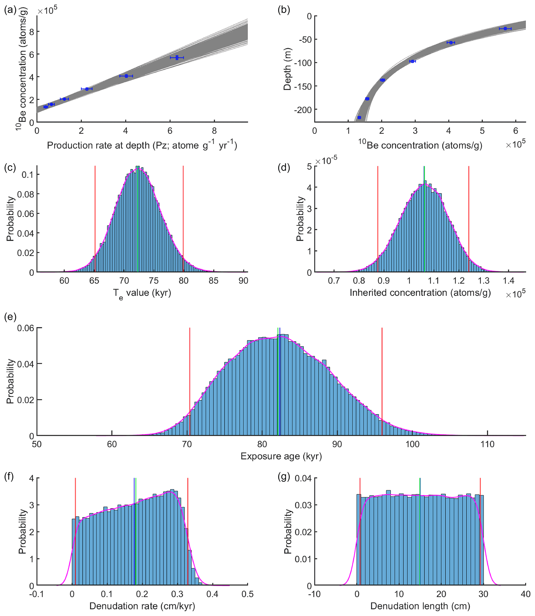
Figure 9 Linear-regression results for Lees Ferry data set with the denudation-depth approach after 100 000 iterations. (a) Relationship of sample concentration to production rate at depth. Grey lines are the best-fit lines for the data. (b) Distribution of depth profile models with best-fit curves (grey lines). (c) Distribution of the effective exposure age (T_e). (d) Distribution of inherited ¹⁰Be concentration. (e) Distribution of exposure age estimates derived from T_e values from linear regression (c). (f) Distribution of denudation rates predicted by the model. (g) Distribution preset of total denudation depth. Red lines indicate 95 % confidence error range, green line indicates the median of the distribution, blue line indicates the mean of the distribution.

Following the original study, we apply our modeling approaches to the sand depth profile data (Table S1). In order to compare with results reported by Hidy et al. (2010), we use the same values they do for all parameters wherever possible (Table S2). Similar to the Beida River depth profile, we estimate the exposure age with the denudation-depth approach, applying Monte Carlo simulation of the uncertainty of input parameters. With a uniformly distributed 0–30 cm denudation length, the inverted best-fit lines and curves are in Fig. 9a and b. The estimated range of T_e and C_inh values are 65.2–79.9 kyr and 8.8–12.4 × 10⁴ atoms g⁻¹, respectively (95 % confidence; Fig. 9c and d). The estimated exposure age is 70.4–96.0 kyr (95 % confidence; Fig. 9e).

4 Discussion

4.1 Case–example comparison

For the Beida River site, comparing the age determined here (108.6–151.3 kyr) to that we reported previously (107.9–164.5 kyr; Wang et al., 2020), the mean is 5 % younger, while the 95 % error range is 24 % smaller. These differences come from three different sources. First, there is a ∼ 1 % shift that arises from independently sampling depth for each measurement (the depth distributions for each sample were not sampled independently in the original paper). Second, the original paper did not take muogenic production into account. The contribution from muons leads to slightly younger age and lowers the inheritance. Third, we applied the denudation-rate approach (Eq. 6) in the 2020 paper, and the corresponding denudation rate distributions are slightly different for the two approaches. Combined, the addition of muogenic contribution and using a denudation-depth instead of denudation-rate approach leads to ∼ 4 % shift of the mean age and to 24 % narrowing of the error range.

For the Lees Ferry site, our age estimation of 70.4–96.0 kyr using the denudation-depth approach generally agrees with the result reported by Hidy et al. (2010), 69.8–103 kyr (or 76.6–96.1 kyr based on recalculation with the updated v1.2 code), though small discrepancies in mean age and 95 % confidence range remain between the two approaches. We suggest this arises from two different sources. First, as demonstrated in Sect. 3.1.1 and Figs. S1–S3, most of the discrepancy may be due to differences between the least-squares and Bayesian model. Secondly, we use a two-term approximation for muogenic process in our model instead of a 5-term approximation used in the original study (Hidy et al., 2010), which may lead to a minor estimation discrepancy.

4.2 Sources of error

4.2.1 Denudation

Denudation and its uncertainty constitute a major source of error in exposure age estimation. With the same surface ¹⁰Be concentration, higher denudation rate and/or larger denudation depth would result in an older effective surface age (e.g., Fig. 1). If a surface is sufficiently old, or if the denudation rate is sufficiently high, the CN build-up at the surface will reach equilibrium with nuclides removed through erosion (Lal, 1991). Figure 10a shows the relationship between denudation rate and surface age (Eq. 7). This figure suggests that once the denudation depth exceeds the mean attenuation length of nucleon spallation $\left(\frac{{\mathrm{\Lambda }}_n}{\mathit{\rho }}\right)$, the slope of the age versus erosion rate relationship degrades the age determination. Once the denudation depth exceeds twice the attenuation length of spallation, the age versus denudation rate curve flattens so much that it becomes effectively impossible to estimate surface age using a denudation-rate approach. On the other hand, the age–denudation depth curve does not flatten as much (Fig. 10b), and therefore it is theoretically possible to use the denudation depth to determine surface age even when total denudation exceeds twice the attenuation length. Our simulated depth profile analysis also shows that the denudation-depth approach can provide accurate estimations even denudation reaches 5 times the spallation attenuation length. In practice, however, surfaces with such a large amount of denudation would subject be to large uncertainties and the denudation history may be too complex for the constant denudation-rate assumption, which underlies both approaches, to be valid, casting doubt on the utility of ¹⁰Be exposure dating for such cases.

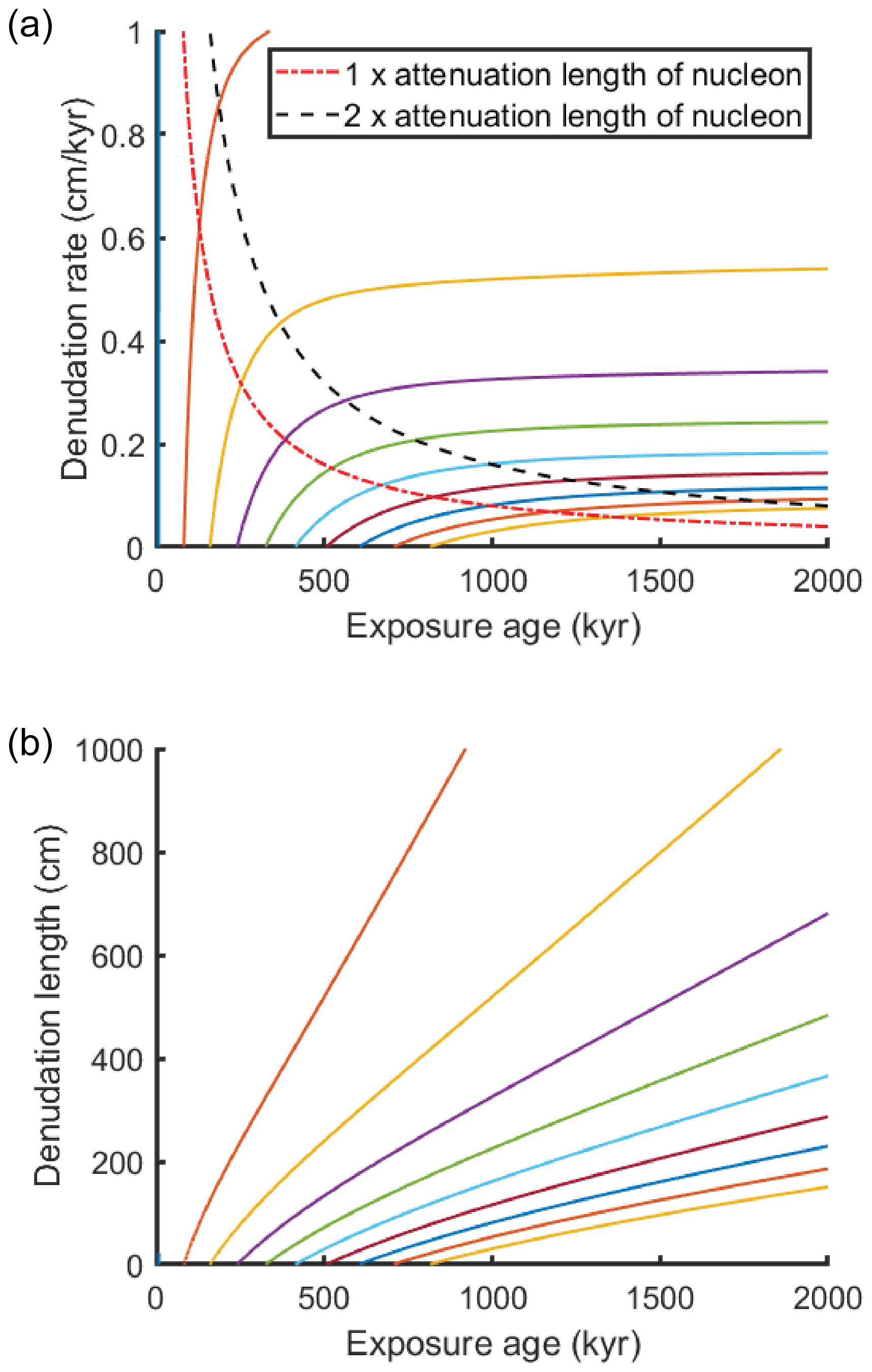
Figure 10 (a) The relationship between denudation rate and exposure age. Each colored line representing the age–denudation relationship of a specific depth profile (or surface concentration). (b) The relationship between denudation depth and exposure age; the color coding matches scenarios shown in (a).

Denudation affects the uncertainty of exposure age estimation in two different ways. First, the uncertainty of the final age increases with denudation rate or depth because of the non-linear relationship between age and denudation (Fig. 10). Second, the age uncertainty will increase further through propagation of the uncertainty of the denudation. This suggests that when excavating depth profile pits in surfaces subject to denudation, it is crucial to document surface texture and analyze the soil profiles to estimate denudation depth, for a small deviation from the true denudation rate or depth would lead to a large bias in the resulting exposure age (Ebert et al., 2012; Frankel et al., 2007; Hidy et al., 2010; Mercader et al., 2012; Ruszkiczay-Rüdiger et al., 2016).

4.2.2 Muogenic production

Muogenic production affects the accuracy of the estimated surface ages differently for the various approaches considered here. For surfaces with no denudation, muons may be fully incorporated into the inversion (Eq. 4); therefore the uncertainty only comes from the uncertainties of parameters related to muogenic production (attenuation length and production rate). When denudation is present, both denudation-rate and denudation-depth approaches come with error related to muons. For the denudation-rate approach, which ignores muons and only models on the relationship between ¹⁰Be concentration and nucleon spallation production rates (Eq. 6), there is a slight overestimation of exposure age and inheritance. This is because the inversion process attributes a small portion of the muogenic concentration to nucleon spallation, and a larger portion is attributed to inheritance. For the denudation-depth approach, there is a negligible error related to the approximate solution for the muogenic contribution (Appendix A).

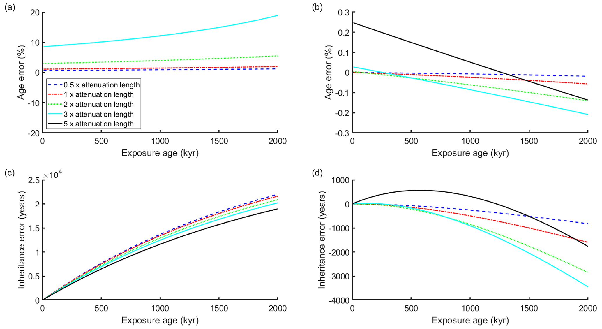
Figure 11 Error vs. exposure age under five different denudation conditions. Each line represents a modeled surface that has undergone various exposure times, but with the same total denudation, expressed as a multiple of the attenuation length, $\frac{\mathit{\rho }}{{\mathrm{\Lambda }}_n}$ for spallation (see legend). (a) Percentage error in exposure age resulting from application of denudation-rate approach. Note that when total erosion reaches 5 times the attenuation length, no meaningful result can be found using this technique. (b) Percentage error in exposure age resulting from application of denudation-depth approach. (c) Error in inheritance, expressed in years based on surface production rate, resulting from application of denudation-rate approach. (d) Error in inheritance, expressed in years based on surface production rate, resulting from application of denudation-depth approach.

To evaluate the error related to muogenic production, we generate profiles with various exposure ages and denudation amounts and compare the estimated results with the true values (Fig. 11). We set the contribution of muogenic production to total surface production as 2 %, though in reality the contribution of muons in most places on earth is smaller (Braucher et al., 2011, 2013; Balco et al., 2008; Balco, 2017); therefore, the errors presented here can be treated as a maximum. We find the error introduced by ignoring muons with the denudation-rate approach is relatively small (less than 2 % and 5 % of overestimate) when the total denudation is under 1 or 2 times the attenuation length for spallation (Fig. 11a). Above 3 times this attenuation length, the error grows drastically until no meaningful result can be found. Compared to the denudation-rate approach, the denudation-depth approach reduces the error by at least 1 order of magnitude (Fig. 11b); even with very large total denudation (5 times the attenuation length), the error is smaller than 0.3 %. Like exposure age, the error in estimated inheritance is related to denudation and exposure age. As demonstrated in Fig. 11c the overestimation of inheritance from the denudation-rate approach increases with the surface age but slightly decreases as the denudation increases. As a comparison, the amount of error from the denudation-depth approach (Fig. 11d) is 1 order of magnitude smaller than the denudation-rate approach.

4.2.3 Other sources of error

Additional sources of error exist for CN depth profile ages that we do not consider in this study. Time-dependent phenomena are not considered. Constant production rate is an important assumption needed to simplify the nuclear build-up process to apply a linear-regression approach. In fact, the production rate is time dependent because the strength of Earth's magnetic field varies with time (Balco, 2017; Desilets et al., 2006; Dunai, 2001; Lifton et al., 2005; Stone, 2000). Extending our model to account for a temporally variable production rate is beyond the scope of the present study. Constant inheritance and a single value for sediment density are other key assumptions for our approach. Sediments sampled from depth profiles are assumed to be well mixed at the time of deposition and to have been deposited rapidly, such that the inherited concentration and density should be the same at every depth. This will not be true for sites with incremental deposition, and for sites where the depositional process or catchment-wide denudation rates vary with time.

5 Conclusions

We introduce a least-squares linear inversion approach to solve cosmogenic nuclide concentration depth profiles for surface exposure age and inheritance, considering denudation rate, denudation depth, and muogenic production. This method allows propagation of error sources using Monte Carlo sampling to infer full probability distributions of age and inheritance. In addition, our model presents a straightforward way to assess the trade-offs between exposure age and denudation rate.

Based on the inversion results of simulated profiles, we show that the least-squares linear regression is a robust approach suitable for most exposure dating scenarios. The accuracy of linear inversion is comparable to a forward Monte Carlo modeling approach for most circumstances, except for the more deviated (noisier) sample sets. Importantly, neither inversion approach consistently outperforms the other. For surfaces with low inheritance or age, as demonstrated with the Beida River sample site and the simulated profiles, unconstrained inversion could lead to incorrect distributions for inversion results. Therefore, the linear regression we proposed here requires applying the nonnegative constraint on such depth profile data.

For surfaces with no denudation, the inversion in Eq. (4) provides an exact solution. For surfaces with denudation, the approximation of muogenic production using the denudation-depth approach (Eq. 10) introduces negligible error even for surfaces with a large amount of denudation. The denudation-rate approach (Eq. 7), though less accurate, provides a useful tool to explore the exposure rate vs. denudation rate relationship. Examples of deep profiles suggest that the linear inversion approach works equally well for samples that were collected deeper than 2 m from the surface, with or without denudation. However, extra caution is needed when collecting and analyzing deep samples to minimize measurement error, as the resulting ages are much more sensitive to the scatter of concentration values relative to near-surface profiles.

Regardless of whether employing linear regression or a forward approach, surfaces that have undergone a large amount of denudation will be subject to large uncertainties related to the denudation rate or depth. It also becomes more tenuous in such cases to assume that the denudation rate was constant throughout the history of the deposit. It is entirely possible that a sample site may have experienced episodic erosional episodes instead of constant denudation rate, which would lead to errors in the age not accounted for in the methods described here.

Appendix A

When ε>0, the effective exposure age T_e takes the following form:

$$\begin{array}{}\text{(A1)}& \begin{array}{rl}& T_{ei}=\left({\displaystyle \frac{\mathrm{1}-e^{-\left(\frac{\mathit{\rho }\mathit{\epsilon }}{{\mathrm{\Lambda }}_i}+\mathit{\lambda }\right)t}}{\frac{\mathit{\rho }\mathit{\epsilon }}{{\mathrm{\Lambda }}_i}+\mathit{\lambda }}}\right)={\displaystyle \frac{\mathrm{1}-e^{-B_{i}t}}{B_i}},\\ & B_i={\displaystyle \frac{\mathit{\rho }\mathit{\epsilon }}{{\mathrm{\Lambda }}_i}}+\mathit{\lambda },i=n,m_{\mathrm{1}},m_{\mathrm{2}}.\end{array}\end{array}$$

This suggests values for T_e value are functions of both ε and t for different production pathways. Between the two variables, ε may be known, while t is unknown. Therefore, our aim is to rewrite Eq. A1 into an approximate form where t can be isolated.

We first take a natural logarithm of the T_em over T_en ratio:

$$\begin{array}{}\text{(A2)}& \begin{array}{rl}\ln \left({\displaystyle \frac{T_{em}}{T_{en}}}\right)& =\ln \left({\displaystyle \frac{\frac{\mathrm{1}-e^{-B_{m}t}}{B_m}}{\frac{\mathrm{1}-e^{-B_{n}t}}{B_n}}}\right)=\ln \left({\displaystyle \frac{\frac{\mathrm{1}-e^{-B_{m}t}}{B_{m}t}}{\frac{\mathrm{1}-e^{-B_{n}t}}{B_{n}t}}}\right)\\ & =\ln \left({\displaystyle \frac{\mathrm{1}-e^{-B_{m}t}}{B_{m}t}}\right)-\ln \left({\displaystyle \frac{\mathrm{1}-e^{-B_{n}t}}{B_{n}t}}\right).\end{array}\end{array}$$

The expansion of a function, $f\left(x\right)=\ln \left(\frac{\mathrm{1}-e^{-x}}{x}\right)$, x=B_it, in Eq. (A2) may be achieved by writing a Maclaurin series with the following form:

$$\begin{array}{}\text{(A3)}& f\left(x\right)=f\left(\mathrm{0}\right)+f^{\prime }\left(\mathrm{0}\right)x+{\displaystyle \frac{f^{\prime \prime }\left(\mathrm{0}\right)}{\mathrm{2}\mathrm{!}}}{x}^{\mathrm{2}}+\mathrm{\dots }{\displaystyle \frac{f^{\left(k\right)}\left(\mathrm{0}\right)}{k\mathrm{!}}}{x}^k+\mathrm{\dots }\end{array}$$

To write the expansion, we first rewrite f(x) as

$$\begin{array}{}\text{(A4)}& \begin{array}{rl}f\left(x\right)& =\ln \left({\displaystyle \frac{\mathrm{1}-e^{-x}}{x}}\right)\\ & =\ln \left({\displaystyle \frac{\mathrm{1}-\left(\mathrm{1}-x+\frac{x^{\mathrm{2}}}{\mathrm{2}\mathrm{!}}-\frac{x^{\mathrm{3}}}{\mathrm{3}\mathrm{!}}+\frac{x^{\mathrm{4}}}{\mathrm{4}\mathrm{!}}-\mathrm{\dots }\right)}{x}}\right)\\ & =\ln \left(\mathrm{1}-{\displaystyle \frac{x}{\mathrm{2}\mathrm{!}}}+{\displaystyle \frac{x^{\mathrm{2}}}{\mathrm{3}\mathrm{!}}}-{\displaystyle \frac{x^{\mathrm{3}}}{\mathrm{4}\mathrm{!}}}+\mathrm{\dots }\right).\end{array}\end{array}$$

In this form, f(x) goes to zero when x goes to zero, and therefore we have

$$\begin{array}{}\text{(A5a)}& f\left(\mathrm{0}\right)=\ln \left(\mathrm{1}\right)=\mathrm{0}\end{array}$$

$$f^{\prime }\left(x\right)={\displaystyle \frac{-\frac{\mathrm{1}}{\mathrm{2}}+\frac{x}{\mathrm{3}}-\frac{x^{\mathrm{2}}}{\mathrm{8}}+\mathrm{\dots }}{\mathrm{1}-\frac{x}{\mathrm{2}\mathrm{!}}+\frac{x^{\mathrm{2}}}{\mathrm{3}\mathrm{!}}-\frac{x^{\mathrm{3}}}{\mathrm{4}\mathrm{!}}+\mathrm{\dots }}}$$

and

$$\begin{array}{}\text{(A5b)}& f^{\prime }\left(\mathrm{0}\right)={\displaystyle \frac{-\frac{\mathrm{1}}{\mathrm{2}}}{\mathrm{1}}}=-{\displaystyle \frac{\mathrm{1}}{\mathrm{2}}}\end{array}$$

$$\begin{array}{rl}& f^{\prime \prime }\left(x\right)\left(\mathrm{1}-{\displaystyle \frac{x}{\mathrm{2}\mathrm{!}}}+{\displaystyle \frac{x^{\mathrm{2}}}{\mathrm{3}\mathrm{!}}}-{\displaystyle \frac{x^{\mathrm{3}}}{\mathrm{4}\mathrm{!}}}+\mathrm{\dots }\right)\\ & +f^{\prime }\left(x\right)\left(-{\displaystyle \frac{\mathrm{1}}{\mathrm{2}}}+{\displaystyle \frac{x}{\mathrm{3}}}-{\displaystyle \frac{x^{\mathrm{2}}}{\mathrm{8}}}+\mathrm{\dots }\right)={\displaystyle \frac{\mathrm{1}}{\mathrm{3}}}-{\displaystyle \frac{x}{\mathrm{4}}}+\mathrm{\dots }\end{array}$$

and

$$\begin{array}{}\text{(A5c)}& f^{\prime \prime }\left(\mathrm{0}\right)={\displaystyle \frac{\mathrm{1}}{\mathrm{12}}}.\end{array}$$

We omit higher-order derivatives from the series expansion.

Bringing Eq. (A5) into Eq. (A3), we have the expansion of f(x) as

$$\begin{array}{}\text{(A6)}& f\left(x\right)=-{\displaystyle \frac{x}{\mathrm{2}}}+{\displaystyle \frac{x^{\mathrm{2}}}{\mathrm{24}}}+O\left(x^{\mathrm{3}}\right).\end{array}$$

Bringing Eq. (A6) into Eq. (A2), the natural logarithm of T_em over T_en ratio is

$$\begin{array}{}\text{(A7)}& \begin{array}{rl}\ln \left({\displaystyle \frac{T_{em}}{T_{en}}}\right)=& \ln \left({\displaystyle \frac{\frac{\mathrm{1}-e^{-B_{m}t}}{B_m}}{\frac{\mathrm{1}-e^{-B_{n}t}}{B_n}}}\right)\\ =& \ln \left({\displaystyle \frac{\mathrm{1}-e^{-B_{m}t}}{B_{m}t}}\right)-\ln \left({\displaystyle \frac{\mathrm{1}-e^{-B_{n}t}}{B_{n}t}}\right)\\ =& -{\displaystyle \frac{B_{m}t}{\mathrm{2}}}+{\displaystyle \frac{{\left(B_{m}t\right)}^{\mathrm{2}}}{\mathrm{24}}}-\left(-{\displaystyle \frac{B_{n}t}{\mathrm{2}}}+{\displaystyle \frac{{\left(B_{n}t\right)}^{\mathrm{2}}}{\mathrm{24}}}\right)\\ & +\left(O\left({\left(B_{m}t\right)}^{\mathrm{3}}\right)-O\left((B_{n}t{)}^{\mathrm{3}}\right)\right).\end{array}\end{array}$$

The contribution of the third term, t³, is negligible and may be neglected. Making the substitution D = εt, the first-order terms in Eq. (A7),

$$\begin{array}{}\text{(A8)}& \begin{array}{rl}-{\displaystyle \frac{B_{m}t}{\mathrm{2}}}+{\displaystyle \frac{B_{n}t}{\mathrm{2}}}& =-{\displaystyle \frac{\mathrm{1}}{\mathrm{2}}}\left({\displaystyle \frac{\mathit{\rho }D}{{\mathrm{\Lambda }}_m}}+\mathit{\lambda }t-{\displaystyle \frac{\mathit{\rho }D}{{\mathrm{\Lambda }}_n}}-\mathit{\lambda }t\right)\\ & =-{\displaystyle \frac{\mathrm{1}}{\mathrm{2}}}\left({\displaystyle \frac{\mathit{\rho }D}{{\mathrm{\Lambda }}_m}}-{\displaystyle \frac{\mathit{\rho }D}{{\mathrm{\Lambda }}_n}}\right).\end{array}\end{array}$$

This result is independent on the exposure age, t.

With the same substitution, the second-order terms in Eq. (A7),

$$\begin{array}{}\text{(A9)}& \begin{array}{rl}& {\displaystyle \frac{{\left(B_{m}t\right)}^{\mathrm{2}}}{\mathrm{24}}}-{\displaystyle \frac{{\left(B_{n}t\right)}^{\mathrm{2}}}{\mathrm{24}}}\\ =& {\displaystyle \frac{\mathrm{1}}{\mathrm{24}}}\left[{\left({\displaystyle \frac{\mathit{\rho }D}{{\mathrm{\Lambda }}_m}}+\mathit{\lambda }t\right)}^{\mathrm{2}}-{\left({\displaystyle \frac{\mathit{\rho }D}{{\mathrm{\Lambda }}_n}}+\mathit{\lambda }t\right)}^{\mathrm{2}}\right]\\ =& {\displaystyle \frac{\mathrm{1}}{\mathrm{24}}}\left[{\left({\displaystyle \frac{\mathit{\rho }D}{{\mathrm{\Lambda }}_m}}\right)}^{\mathrm{2}}+{\displaystyle \frac{\mathrm{2}\mathit{\rho }D\mathit{\lambda }t}{{\mathrm{\Lambda }}_m}}+{\left(\mathit{\lambda }t\right)}^{\mathrm{2}}-{\left({\displaystyle \frac{\mathit{\rho }D}{{\mathrm{\Lambda }}_n}}\right)}^{\mathrm{2}}\right.\\ & \left.-{\displaystyle \frac{\mathrm{2}\mathit{\rho }D\mathit{\lambda }t}{{\mathrm{\Lambda }}_n}}-{\left(\mathit{\lambda }t\right)}^{\mathrm{2}}\right]\\ =& {\displaystyle \frac{\mathrm{1}}{\mathrm{24}}}\left[{\left({\displaystyle \frac{\mathit{\rho }D}{{\mathrm{\Lambda }}_m}}\right)}^{\mathrm{2}}-{\left({\displaystyle \frac{\mathit{\rho }D}{{\mathrm{\Lambda }}_n}}\right)}^{\mathrm{2}}\right]\\ & +{\displaystyle \frac{\mathrm{1}}{\mathrm{24}}}\left[{\displaystyle \frac{\mathrm{2}\mathit{\rho }D\mathit{\lambda }t}{{\mathrm{\Lambda }}_m}}-{\displaystyle \frac{\mathrm{2}\mathit{\rho }D\mathit{\lambda }t}{{\mathrm{\Lambda }}_n}}\right].\end{array}\end{array}$$

In Eq. (A9), the first term of the right-hand side is independent of age, t, while the second term is dependent of age. We therefore choose to omit the second term of Eq. (A9) in order to develop an age-independent approximation. We find that this term may be omitted for two reasons. First, the absolute value of Eq. (A8) is at least 1 order of magnitude larger than Eq. (A9), and therefore omitting one term from Eq. (A9) will not lead to significant decrease in accuracy of the overall approximation. Second, for young surfaces, λt is sufficiently small that the second term of Eq. (A9) is much smaller than the first term, which means omitting it will lead to an even smaller decrease in accuracy.

Therefore, an approximate form of Eq. (A7) that is independent of t is

$$\begin{array}{}\text{(A10)}& \begin{array}{rl}\ln \left({\displaystyle \frac{T_{em}}{T_{en}}}\right)\approx & -{\displaystyle \frac{\mathrm{1}}{\mathrm{2}}}\left({\displaystyle \frac{\mathit{\rho }D}{{\mathrm{\Lambda }}_m}}-{\displaystyle \frac{\mathit{\rho }D}{{\mathrm{\Lambda }}_n}}\right)\\ & +{\displaystyle \frac{\mathrm{1}}{\mathrm{24}}}\left[{\left({\displaystyle \frac{\mathit{\rho }D}{{\mathrm{\Lambda }}_m}}\right)}^{\mathrm{2}}-{\left({\displaystyle \frac{\mathit{\rho }D}{{\mathrm{\Lambda }}_n}}\right)}^{\mathrm{2}}\right],\end{array}\end{array}$$

and the ratio between muon and nucleon effective age can be approximated as

$$\begin{array}{}\text{(A11)}& {\displaystyle \frac{T_{em}}{T_{en}}}\approx e^{-\frac{\mathrm{1}}{\mathrm{2}}\left(\frac{\mathit{\rho }D}{{\mathrm{\Lambda }}_m}-\frac{\mathit{\rho }D}{{\mathrm{\Lambda }}_n}\right)+\frac{\mathrm{1}}{\mathrm{24}}\left[{\left(\frac{\mathit{\rho }D}{{\mathrm{\Lambda }}_m}\right)}^{\mathrm{2}}-{\left(\frac{\mathit{\rho }D}{{\mathrm{\Lambda }}_n}\right)}^{\mathrm{2}}\right]}.\end{array}$$