ChronoLorica: introduction of a soil–landscape evolution model combined with geochronometers

Understanding long-term soil and landscape evolution can help us understand the threats to current-day soils, landscapes and their functions. The temporal evolution of soils and landscapes can be studied using geochronometers, such as optically stimulated luminescence (OSL) particle ages or radionuclide inventories. Also, soil–landscape evolution models (SLEMs) can be used to study the spatial and temporal evolution of soils and landscapes through numerical modelling of the processes responsible for the evolution. SLEMs and geochronometers have been combined in the past, but often these couplings focus on a single geochronometer, are designed for specific idealized landscape positions, or do not consider multiple transport processes or post-depositional mixing processes that can disturb the geochronometers in sedimentary archives.

We present ChronoLorica, a coupling of the soil–landscape evolution model Lorica with a geochronological module. The module traces spatiotemporal patterns of particle ages, analogous to OSL ages, and radionuclide inventories during the simulations of soil and landscape evolution. The geochronological module opens rich possibilities for data-based calibration of simulated model processes, which include natural processes, such as bioturbation and soil creep, as well as anthropogenic processes, such as tillage. Moreover, ChronoLorica can be applied to transient landscapes that are subject to complex, non-linear boundary conditions, such as land use intensification, and processes of post-depositional disturbance which often result in complex geo-archives.

In this contribution, we illustrate the model functionality and applicability by simulating soil and landscape evolution along a two-dimensional hillslope. We show how the model simulates the development of the following three geochronometers: OSL particle ages, meteoric ¹⁰Be inventories and in situ ¹⁰Be inventories. The results are compared with field observations from comparable landscapes. We also discuss the limitations of the model and highlight its potential applications in pedogenical, geomorphological or geological studies.

1 Introduction

Soils and landscapes have been affected by climate change and human use for over thousands of years (Rothacker et al., 2018; Stephens et al., 2019), leading to soil degradation in the form of soil erosion, soil carbon losses and nutrient losses (Sanderman et al., 2017; Olsson et al., 2019). Since the industrial revolution, these degradation processes have been greatly amplified due to deforestation, intensive land management and more extreme weather. Knowledge of the long-term rates and extents of these degradation processes is required to understand the threats to current-day soils, landscapes and their functions.

In eroding and depositionary landscapes, soil material is detached, transported and deposited by natural and anthropogenic processes. These sedimentary deposits provide archives that can be used to derive phases and rates of landscape change, which are essential to understand past and present landscape dynamics (Dotterweich, 2008). There are various methods to study the erosion and sediment dynamics in eroding landscapes. One method is based on soil particles building up an optically stimulated luminescence (OSL) signal that is reset when the particle is exposed to daylight and is recharged by ionizing radiation in the subsurface when shielded from daylight (Wallinga et al., 2019). This OSL signal acts as a proxy for the duration of burial of the layer in which the soil particle is located. Another method uses radionuclides, which are rare radioactive isotopes that form or accumulate in soils and sediments. The two- or three-dimensional distribution patterns of these radionuclides can be used to calculate soil erosion or deposition rates and even bedrock erosion rates (Ritchie and McHenry, 1990; Brown et al., 1995; Heimsath et al., 1997). Examples of radionuclides are cosmic-ray-produced nuclides, such as ¹⁰Be ($t_{\mathrm{1}/\mathrm{2}}=\mathrm{1.39}$ Ma) or ¹⁴C ($t_{\mathrm{1}/\mathrm{2}}=\mathrm{5.7}$ ka; Lal, 1991; Ivy-Ochs and Kober, 2008), and fallout radionuclides, such as ¹³⁷Cs ($t_{\mathrm{1}/\mathrm{2}}=\mathrm{30}$ a) or ^239+240Pu ($t_{\mathrm{1}/\mathrm{2}}$ = 24.1 and 6.55 ka), that are released after nuclear accidents and bomb tests (Ketterer et al., 2004; Alewell et al., 2017). Depending on their half-life, different radionuclides provide information on processes that act over different timescales. Therefore, both OSL signals and radionuclides are the basis for geochronometers that can be used for studying lateral sediment transport processes, as well as vertical soil-mixing processes (Brown et al., 2003; Arata et al., 2016a, b; Gray et al., 2019; Román-Sánchez et al., 2019b). They are used in experimental studies (Stockmann et al., 2013; Gliganic et al., 2015), as well as in numerical studies (Furbish et al., 2018b; Campforts et al., 2016; Johnson et al., 2014).

However, there are settings where geochronometers are not immediately suitable for studying soil and landscape change. This is, for example, the case in landscapes where sedimentary archives are partially disturbed (e.g. Van der Meij et al., 2019) or absent, where the sedimentary material is unsuitable for geochronological methods, or where individual process signals cannot be derived from complex geo-archives which formed under multiple, often non-linear, processes (Temme et al., 2015). In other cases, existing geochronological methods rely on assumptions that are not valid for the landscape studied. For example, most analytical methods for radionuclides assume steady-state conditions in a landscape (Heimsath et al., 1997). This assumption is not always true, certainly not in landscapes that are subject to changing erosion rates and anthropogenic disturbances, such as agricultural landscapes (Willenbring and von Blanckenburg, 2010; Mudd, 2017; Hippe et al., 2021). In these transient landscapes, sudden or non-linear changes in environmental drivers, such as land use intensification, cause landscapes, soils and geochronometers to change at rates much higher than those that occur under natural conditions, which often leads to divergent development of the soil and landscape properties (Sommer et al., 2008; Van der Meij, 2022).

In these cases, it should be useful to directly simulate the transport and mixing processes of geochronometers using numerical computer models, specifically soil–landscape evolution models (SLEMs). SLEMs are models that simulate pedogenical and geomorphological processes that are responsible for spatial and temporal soil and landscape development, driven by various internal and external drivers (Minasny et al., 2015; Van der Meij et al., 2018). By simultaneously considering pedogenical and geomorphological processes, interactions and co-evolution of soils and landscapes can be simulated. SLEMs have the advantage that they provide continuous, landscape-wide soil and landscape properties in three dimensions as opposed to field measurements that are typically limited in space. Also, such models provide changes in these properties over time, where measurements often are taken at one point in time or over a very short time span or may average rates over excessively long timescales relative to the processes that are studied (Van der Meij, 2022). This four-dimensional representation of the soil–landscape system enables the study of lateral and vertical soil and geomorphological processes, including the development of sedimentary archives, albeit in a hypothetical and simplified simulation.

SLEMs have successfully been combined with radionuclide methods to parametrize and calibrate process rates and to increase our understanding of soil and landscape change. For example, SPEROS-C and derived models are calibrated with fallout isotopes to study recent anthropogenic erosion processes (Van Oost et al., 2003, 2005; Wilken et al., 2020), Be2D studies the mobility of meteoric ¹⁰Be by simulating vertical and lateral mixing and transport processes (Campforts et al., 2016), and Anderson (2015) and Furbish et al. (2018a, b) developed models (not strictly SLEMs) that study the distribution of cosmogenic nuclides and OSL particle ages due to transport and mixing processes on hillslopes. Individual soil processes can also be calibrated using geochronometers, for example clay translocation (Jagercikova et al., 2015) and bioturbation (Wilkinson and Humphreys, 2005; Johnson et al., 2014; Román-Sánchez et al., 2019b). SLEMs combined with geochronometers, however, often focus on a single geochronometer or soil–landscape process; are designed for specific, idealized landscape positions; and/or do not consider secondary processes that might disturb the geochronometers in sediment archives, such as post-depositional mixing by tillage.

In this study, we aim to bridge these limitations by combining SLEMs with geochronometers. We present an extension to the SLEM Lorica (Temme and Vanwalleghem, 2016; Van der Meij et al., 2020), where we coupled various geochronometers to the existing pedogenical and geomorphological processes in the model. With this extended model, named ChronoLorica, we aim to do the following:

1. calibrate pedogenical and geomorphological processes in the model using measured geochronometers

2. study the effect of natural and anthropogenic soil transport and mixing processes on the chronological information present in soils and sediment archives

3. understand soil and landscape evolution in transient agricultural landscapes that are subject to complex boundary conditions, such as intensification of land management.

In this paper, we introduce ChronoLorica and show its potential for unravelling chronologies and landscape evolution in transient landscapes. First, we describe the geochronological module of ChronoLorica. Second, we simulate several soil and landscape processes to show how chronologies can develop in natural and transient agricultural landscapes. Third, we discuss the added value of coupling soil–landscape evolution modelling with geochronometers, the model limitations and potential applications of the model in soil, geomorphological or geological studies.

2 Model description

2.1 Model architecture

ChronoLorica is an extension to the soil–landscape evolution model Lorica (Temme and Vanwalleghem, 2016). In Lorica, the relief of a landscape is represented by a raster-based digital elevation model (DEM), which controls the overland routing of water. The elevation of each raster cell can be modified by removal or addition of soil material by various geomorphological and pedogenical processes. Soils are represented by a pre-defined number of soil layers below each raster cell. Lorica works with a dynamic adaptation of the number and thickness of soil layers, enabling more detail in heterogeneous sections and less detail in homogeneous sections of the soil. Inside these layers, the model keeps track of five texture classes (coarse, sand, silt, clay and fine clay) and two organic matter (OM) classes (old and young). The composition of each layer can be modified by geomorphological processes, as well as by pedogenical processes. The soil components are recorded in kilograms and converted to elevation or layer thickness in metres using a pedotransfer function of bulk density (here, we use that of Tranter et al., 2007). The model is therefore based on conservation of mass, where the sum of the mass of all soil components is always equal. This includes soil material that was exported from the modelling domain, for example by deep leaching or overland flow. The dynamic architecture of Lorica makes it suitable for adaptation to locally occurring processes (Van der Meij et al., 2016) or for including additional drivers (HydroLorica, Van der Meij et al., 2020). Lorica and ChronoLorica are written in C#.

2.2 Process descriptions

The pedogenical processes that we included in this study are clay translocation and bioturbation. The pedogenical processes are vertically oriented, meaning that resulting transport occurs only in the vertical direction. The geomorphological processes that are included in this study are tillage mixing and erosion and soil creep. These mechanisms are oriented laterally, leading to detachment, transport and possible deposition of soil material. The associated mixing processes occur vertically. Other processes that are present in the Lorica model but were not included in this study are physical and chemical weathering, carbon cycling, overland flow, and tree throw (Temme and Vanwalleghem, 2016; Van der Meij et al., 2020). For some of these, the geochronological module is not developed yet.

These processes can be considered to be advective, diffusive or transformative. Advective processes trigger directional movements of soil matter, often driven by water flow, leading to heterogeneity in topography or development of soil horizons. Diffusive processes homogenize soil layers or topography, for example by mixing. Transformative processes transform soil particles into other particles, for example by breaking down as a result of weathering. The mathematical descriptions of these processes follow advective and diffusive formulations that are often used in numerical particle transport models (e.g. Anderson, 2015; Furbish et al., 2018a), with the difference being that the processes in Lorica are programmed as distinct processes that affect the bulk soil rather than individual particles. These changes, in turn, affect multiple soil and landscape properties and the geochronometers that are introduced in the next Section.

Below, we describe the processes that were simulated in this study. For those whose rates change with soil depth, we use an exponential depth function. This shape is found in many soil processes and properties (Minasny et al., 2016), including soil creep (Roering, 2004). It represents diminishing temperature and soil moisture variations with depth (Amenu et al., 2005), diminishing biological activity for some organisms (Canti, 2003), and the root distributions of some plants (Gregory, 2006). However, as these references also state, this exponential profile is not valid for all settings because there can be different organisms and processes responsible for soil mixing and transport. For each application of the model, the processes, depth functions and parameters should be derived from field data or comparable studies.

Soil creep is simulated as a diffusive geomorphological process that leads to gradual smoothing of the surface. Soil material is transported between soil layers of adjacent cells. The amount of soil material creeping out of a cell towards a lower-lying neighbouring cell, CR_local [kg a⁻¹], is calculated by multiplying the potential amount of creep CR_pot [kg a⁻¹] with an exponential depth decay function over the soil depth sd [m] and the local slope gradient Λ_local [m m⁻¹]. The resulting value is then multiplied by the division of Λ_local to the power of the convergence factor p [–], divided by the sum of slope gradients to the power of p towards all lower-lying neighbouring cells (Eq. 1). This last part of the equation controls the diffusive transport through the landscape using the multiple-flow algorithm (Freeman, 1991). The parameter p determines the division of the transport over all lower-lying neighbouring cells. With higher values of p, transport becomes more convergent towards the lowest neighbouring cell. This equation differs from earlier reported process descriptions in Lorica (Van der Meij et al., 2020). The shape of the depth decay function is controlled by the depth decay rate for creep dd_CR [m⁻¹]. CR_local is divided over all soil layers at the source location, proportionally to the fraction of the integral of the depth decay function over the upper and lower depths (z_upper, z_lower) [m] of the respective layer, divided by the integral of the depth decay function over the entire soil column (Eq. 2). The resulting CR_layer [kg a⁻¹] is the total amount of mass leaving a soil layer. This mass is gathered from all fine-texture fractions (i.e. excluding the fraction coarser than sand) relative to the texture distribution. The mass is transported to adjacent soil layers in the receiving cell. When multiple receiving layers neighbour the source layer, CR_layer is distributed proportionally to the size of the shared boundaries.

$$\begin{array}{}\text{(1)}& {\displaystyle }{\mathrm{CR}}_{\mathrm{local}}={\mathrm{CR}}_{\mathrm{pot}}\cdot \left(\mathrm{1}-e^{-{\mathrm{dd}}_{\mathrm{CR}}\cdot \mathrm{sd}}\right)\cdot {\mathrm{\Lambda }}_{\mathrm{local}}\cdot {\displaystyle \frac{{\mathrm{\Lambda }}_{\mathrm{local}}^p}{{\sum }_j^J{\mathrm{\Lambda }}_j^p}}\text{(2)}& {\displaystyle }{\mathrm{CR}}_{\mathrm{layer}}={\mathrm{CR}}_{\mathrm{local}}\cdot {\displaystyle \frac{{\int }_{z_{\mathrm{upper}}}^{z_{\mathrm{lower}}}\left(e^{-{\mathrm{dd}}_{\mathrm{CR}}\cdot z}\right)}{{\int }_{\mathrm{0}}^{\mathrm{sd}}\left(e^{-{\mathrm{dd}}_{\mathrm{CR}}\cdot z}\right)}}\end{array}$$

Tillage consists of the following two parts: homogenization of the topsoil and transport of soil material. All soil layers that are located in the range of the plough depth pd [m] are completely mixed with each other in every time step, where layers that are partially in the plough layer contribute a fraction to the mixture. Local tillage transport TI_local [m] is calculated in a similar way as creep, namely by multiplying a tillage constant C_til [a⁻¹] with Λ_local to the power of p divided by the sum of all slope gradients to the power p and the plough depth pd [m] (Eq. 3). TI_local is calculated in metres per year. The ratio between TI_local and the thickness of each possibly eroding soil layer is used to determine the fraction of soil material that can be eroded out of that layer. The eroded material is usually taken from the topmost layer but can be taken from subsequent layers as well when the eroded thickness exceeds the thickness of the top layer.

$$\begin{array}{}\text{(3)}& {\mathrm{TI}}_{\mathrm{local}}=C_{\mathrm{til}}\cdot {\displaystyle \frac{{\mathrm{\Lambda }}_{\mathrm{local}}^p}{{\sum }_j^J{\mathrm{\Lambda }}_j^p}}\cdot {\mathrm{\Lambda }}_{\mathrm{local}}\cdot \mathrm{pd}\end{array}$$

Clay translocation is calculated using an advection equation, similarly to Jagercikova et al. (2015). Bioturbation (see next paragraph) serves as the diffusive part of the process. The translocation of clay from a certain soil layer, CT_layer [kg a⁻¹], is calculated by multiplying the advection parameter CT_adv [m a⁻¹] with a depth decay function, containing the depth decay parameter dd_CT [m⁻¹] and the depth of the layer z_layer [m], the clay fraction of that layer fclay_layer [–], the bulk density of that layer BD_layer [kg m⁻³], and the cell area dx² [m²] (Eq. 4). The translocated clay is transported to the underlying layer or, in the case of the lowest layer, is lost from the soil column. Not all clay in the soil is available for transport. We used the equation of Brubaker et al. (1992) to estimate the fraction of clay that is water dispersible, i.e. available for translocation (fclay_wd, Eq. 5). We estimated the cation exchange capacity (CEC) of each layer, CEC_layer, which is required for the equation of Brubaker, using a pedotransfer function from Ellis and Foth (1996), using the clay fraction fclay_layer and the organic matter fraction fOM_layer in the respective layers (Eq. 6). The latter is 0 in our simulations because we did not simulate the soil organic matter cycle.

$$\begin{array}{}\text{(4)}& {\displaystyle }{\mathrm{CT}}_{\mathrm{layer}}={\mathrm{CT}}_{\mathrm{adv}}\cdot e^{-{\mathrm{dd}}_{\mathrm{CT}}\cdot z_{\mathrm{layer}}}\cdot {\mathrm{fclay}}_{\mathrm{layer}}\cdot {\mathrm{BD}}_{\mathrm{layer}}\cdot {\mathrm{dx}}^{\mathrm{2}}\text{(5)}& {\displaystyle }\begin{array}{rl}{\mathrm{fclay}}_{\mathrm{wd}}& =\mathrm{0.01}\cdot (\mathrm{0.369}\cdot {\mathrm{fclay}}_{\mathrm{layer}}\cdot \mathrm{100}\\ & -\mathrm{8.96}\cdot {\displaystyle \frac{{\mathrm{CEC}}_{\mathrm{layer}}}{{\mathrm{fclay}}_{\mathrm{layer}}\cdot \mathrm{100}}}+\mathrm{4.48})\end{array}\text{(6)}& {\displaystyle }\begin{array}{rl}{\mathrm{CEC}}_{\mathrm{layer}}& =\mathrm{0.1}\cdot (\mathrm{32}+\mathrm{3670}\cdot {\displaystyle \frac{{\mathrm{fOM}}_{\mathrm{layer}}}{\mathrm{1.72}}}\\ & +\mathrm{196}\cdot {\mathrm{fclay}}_{\mathrm{layer}})-\mathrm{300}\cdot {\displaystyle \frac{{\mathrm{fOM}}_{\mathrm{layer}}}{\mathrm{1.72}}}\end{array}\end{array}$$

Bioturbation is calculated as a diffusive process mixing the soil. The total amount of bioturbation at a certain location BT_local [kg a⁻¹] is calculated by multiplying the potential bioturbation BT_pot [kg a⁻¹] with a depth decay function that contains the depth decay parameter for bioturbation dd_BT [m⁻¹] and the local soil depth sd (Eq. 7). The local amount of bioturbation is divided over all soil layers at that location, proportional to the fraction of the integral of the depth decay function over the upper and lower depths (z_upper, z_lower) of the respective layer, divided by the integral of the depth decay function over the entire soil column (Eq. 8), similarly to the creep calculations. The resulting layer bioturbation, BT_layer [kg a⁻¹], is the amount of mass that is exchanged with the respective layer. The exchange occurs with all other layers, but the amount of exchange decreases exponentially with distance from the source layer. For this exponential function, we use a depth decay constant of 2 times the dd_BT to limit the distance over which soil material is mixed. BT_layer is derived from all fine soil textures and organic matter classes, proportional to their fractions in the soil.

$$\begin{array}{}\text{(7)}& {\displaystyle }{\mathrm{BT}}_{\mathrm{local}}={\mathrm{BT}}_{\mathrm{pot}}\cdot \left(\mathrm{1}-e^{-{\mathrm{dd}}_{\mathrm{BT}}\cdot \mathrm{sd}}\right)\text{(8)}& {\displaystyle }{\mathrm{BT}}_{\mathrm{layer}}={\mathrm{BT}}_{\mathrm{local}}\cdot {\displaystyle \frac{{\int }_{z_{\mathrm{upper}}}^{z_{\mathrm{lower}}}\left(e^{-{\mathrm{dd}}_{\mathrm{BT}}\cdot z}\right)}{{\int }_{\mathrm{0}}^{\mathrm{sd}}\left(e^{-{\mathrm{dd}}_{\mathrm{BT}}\cdot z}\right)}}\end{array}$$

2.3 Geochronometers

We built in two types of geochronometers in Lorica. These are the burial ages of individual soil particles, analogous to OSL ages, and the inventories of various cosmogenic nuclides.

2.3.1 OSL particle ages

OSL dating determines the last exposure of a soil particle to daylight, i.e. the moment of bleaching. This is helpful for determining the time of burial of a sediment layer or for determining the rate at which surface particles are mixed in the subsoil. The OSL age is determined by dividing the radiation dose received by a subsample of soil or sediment particle(s) (termed palaeodose [Gy]) by the ionizing radiation from the surrounding soil, sediments and cosmic rays (termed dose rate [Gy ka⁻¹]). OSL ages can be determined for bulk sample material or for smaller amounts of material, down to even single grains of sand (Duller, 2008).

Chronolorica's OSL particle age module keeps track of the erosion, transport and bleaching of a small number of particles in each soil layer through time. Because of this, the intermediate steps of determining palaeodoses and dose rates can be skipped, and the ages of individual particles are traced directly. By tracing the ages of individual particles, we are able to derive their age proxies, which can be translated into probability density functions (PDFs) of OSL particle ages for each soil layer in the model. These PDFs can be compared with measured OSL age PDFs for calibration and validation purposes.

The number of particles in each soil layer varies over space and time due to transport and mixing processes. The redistribution of the particles currently follows the redistribution of the sand fraction in the model, which is the texture class that is typically targeted for single-grain OSL dating (Duller, 2008). The probability that a certain particle is transported together with the transported sand, P_transport, is equal to the transported mass of sand divided by the total mass of sand in the source layer (Eq. 9). This transport probability is then used to randomly assess for each particle whether it will be transported or not. In the case where an entire layer is eroded, P_transport is 1, and all particles will be transported. In the case where only 0.1 % of the sand is transported, there is a probability of 0.1 % for each particle that it will be transported as well.

$$\begin{array}{}\text{(9)}& P_{\mathrm{transport}}={\displaystyle \frac{\mathrm{sand}\mathrm{transported}\left[\mathrm{kg}\right]}{\mathrm{total}\mathrm{sand}\mathrm{present}\left[\mathrm{kg}\right]}}\end{array}$$

The age of the particles in the model can be set to zero (i.e. the particles can be bleached) when they are located in the top soil layer. Estimates of the depth to which daylight can penetrate the soil to bleach particles range between 1 and 10 mm (Furbish et al., 2018b), which agrees with long-term bleaching depths in rock surfaces (10 mm, Sellwood et al., 2019). With intensive mixing of the topsoil, the bleached particles can be found in abundance over the top 5 to 10 cm of the soil (Wilkinson and Humphreys, 2005). The thickness of the top soil layer is set to the bleaching depth, resulting in a completely bleached upper soil layer. The initial number of particles per layer depends on the sand content of the layer and is provided in particles per kg m⁻² sand. This is necessary to account for varying bulk density with depth, which also changes the sand contents and the transport probabilities of the layers. As an example, a soil layer of 0.05 m with 25 % sand, a bulk density of 1500 kg m⁻³ and four simulated particles per kilogram per square metre of sand will have 0.05 ⋅ 1500 ⋅ 0.25 ⋅ 4 = 75 particles.

ChronoLorica traces three types of ages or particle properties that are useful in soil mixing and erosion studies. The first age is the apparent age, which is the actual age of a particle that is analogous to an OSL-measured age. This is the age of the particle that is reset when it is bleached at the surface. Next to that, we also track the depositional age, which is reset when a particle is transported laterally due to surface erosion processes, such as water erosion and tillage erosion. Especially in agricultural systems, tillage is a strong secondary mixing process that can greatly disturb the depositional chronology in colluvial deposits by resurfacing and bleaching particles that may have been deposited a long time ago (Van der Meij et al., 2019). By tracing both the apparent ages and the deposition ages, we can reconstruct depositional chronologies in soil–landscape systems that are significantly impacted by post-depositional mixing. The third property that is traced, the surfaced count, is the number of times a particle has been bleached at the surface.

To illustrate the different processes that affect the particle location and age, we will follow the fate of a hypothetical sand particle in late Pleistocene cover sand. This particle has been deposited near the surface, high up on a gently sloping hillslope. After the landscape stabilized and vegetation started to grow in the Holocene, sands started to get mixed vertically by bioturbation. Our particle reached the surface several times, where it was bleached, before it was mixed back into the subsurface. The apparent age of the particle corresponds to the last moment the particle was exposed to daylight, while the surfaced count keeps track of the number of times the particle has been surfaced. At a certain moment in time, the hillslope is cultivated, and the soils begin to be ploughed. Our particle is located near the surface at that time, so it is incorporated into the plough layer, which has much higher mixing rates than the undisturbed natural soils. In the plough layer, our particle is surfaced several more times, and its apparent age gets reset every time. Next to the intensive mixing, the particle is also transported downslope due to tillage erosion. Every time the particle moves laterally with the eroding topsoil, the deposition age gets reset. Eventually, the particle reaches the foot slope, where it is incorporated into a colluvial layer. The deposition age starts to build up, but the apparent age still gets reset when the particle is surfaced in the plough layer at the location of deposition. Only when the particle is buried below new colluvium and has thus left the active mixing zone can its apparent age increase again. This is the age that can be measured with OSL dating of the colluvium.

Because the particles are transported between multiple soil layers and locations, the number of particles per layer is not constant. With erosion, the number of particles in a layer can decrease, while deposition can increase the number of particles. The tracing of individual particles that vary in number for each location required a memory-intensive implementation in the model. We make use of a three-dimensional jagged array for this purpose. Jagged arrays contain elements that can be variable in length. In practice, this means that, for every row, column and layer in the model, there is an array of OSL particle ages that can vary in length. Because of memory restrictions and computational demands, the number of particles in each layer is limited. This number should depend on the dimensions of the soil landscape that is simulated, the runtime of the model and the specifications of the computer. We will discuss the choice of the initial number of particles in more detail in the discussion.

2.3.2 Cosmogenic nuclides

ChronoLorica records the inventories of various cosmogenic nuclides for each row, column and soil layer in the model. This enables the calculation of the spatial distribution patterns, as well as of the depth functions, of these radionuclides. For each soil layer, the total number of radionuclides is stored as atoms cm⁻². In this contribution, we focus on cosmogenic nuclides. We distinguish externally produced, meteoric cosmogenic nuclides and in-situ-produced cosmogenic nuclides. Each radionuclide in the model behaves similarly, but their dynamics depend on the type of accumulation or production, their decay rate and the soil texture fraction they are associated to. It is likely that there are already radionuclides present at the start of a simulation. Therefore, all radionuclides can have an inherited inventory, which is the number of atoms present at the start of simulations. These inventories are homogeneous throughout the profile.

Meteoric cosmogenic nuclides

Meteoric cosmogenic nuclides are produced in the atmosphere via spallation reactions as a result of the collision of cosmic radiation with atmospheric gases. These nuclides are then delivered to the earth's surface by capture with precipitation (Willenbring and von Blanckenburg, 2010). For ChronoLorica, we use meteoric ¹⁰Be as one of the meteoric geochronometers. In non-acidic soils, meteoric ¹⁰Be binds primarily to clay particles (up to 80 %; Jagercikova et al., 2015). In more acidic soils (pH < 4.1; Graly et al., 2010; Willenbring and von Blanckenburg, 2010), meteoric ¹⁰Be leaches from the soil.

As Lorica is mainly designed for pedogenesis in loamy soils, meteoric ¹⁰Be is a suitable marker for lateral and vertical clay redistribution due to erosion processes, bioturbation and clay translocation (Campforts et al., 2016; Jagercikova et al., 2015). The adsorption of meteoric ¹⁰Be is grain-size dependent, but most of the nuclides adsorb to the clay fraction (Wittmann et al., 2012). To account for this grain-size selectivity, we assign 80 % of the input to be associated with the clay fraction (Jagercikova et al., 2015), while the rest is associated with the silt fraction. Vertical and lateral redistribution of meteoric ¹⁰Be in the model thus follows the redistribution of the clay fraction primarily and the silt fraction secondarily.

In ChronoLorica, the accumulation of meteoric radionuclides follows an exponentially declining rate with soil depth (Willenbring and von Blanckenburg, 2010). The total local input of a meteoric radionuclide, A_me,local [atoms cm⁻² a⁻¹], is calculated by multiplying the potential deposition, A_me,pot [atoms cm⁻² a⁻¹], which is a given input parameter, with a depth decay function that contains the adsorption coefficient for the meteoric cosmogenic nuclide, k_me [m⁻¹], and soil depth sd (Eq. 10). The adsorption coefficient serves the same purpose as the depth decay parameters for the soil processes. The total local input, A_me,local, is divided over all soil layers at that location based on the depth of the respective layer and the depth decay function (Eq. 11). The change in radionuclide inventory in a certain layer is the sum of the current inventory and A_me,layer, multiplied with 1−λ_me to account for radioactive decay (Eq. 12).

$$\begin{array}{}\text{(10)}& {\displaystyle }{A}_{\mathrm{me},\mathrm{local}}=A_{\mathrm{me},\mathrm{pot}}\cdot \left(\mathrm{1}-e^{-k_{\mathrm{me}}\cdot \mathrm{sd}}\right)\text{(11)}& {\displaystyle }{A}_{\mathrm{me},\mathrm{layer}}=A_{\mathrm{me},\mathrm{local}}\cdot {\displaystyle \frac{{\int }_{z_{\mathrm{upper}}}^{z_{\mathrm{lower}}}\left(e^{-k_{\mathrm{me}}\cdot z}\right)}{{\int }_{\mathrm{0}}^{\mathrm{sd}}\left(e^{-k_{\mathrm{me}}\cdot z}\right)}}\text{(12)}& {\displaystyle }{C}_{\mathrm{me},\mathrm{layer},t+\mathrm{1}}=\left(C_{\mathrm{me},\mathrm{layer},t}+A_{\mathrm{me},\mathrm{layer}}\right)\cdot \left(\mathrm{1}-{\mathit{\lambda }}_{\mathrm{me}}\right)\end{array}$$

In situ cosmogenic nuclides

In contrast to meteoric cosmogenic nuclides, in situ cosmogenic nuclides are produced in the soil or in the underlying bedrock itself. Two examples of in situ cosmogenic nuclides are in situ ¹⁰Be and in situ ¹⁴C. Due to the long half-life of ¹⁰Be, this isotope is suitable for tracing both short- and long-term soil–landscape processes (10²–10⁷ a). The shorter half-life of ¹⁴C makes it more suitable for tracing Holocene soil–landscape processes (10²–10⁴ a; Walker, 2005). Within the uppermost few metres from the surface, most in situ cosmogenic nuclides are formed due to penetrating cosmic radiation rays causing nuclear spallation of target elements, such as O in quartz, the mineral most commonly used for in situ ¹⁰Be and ¹⁴C. Formation of in situ cosmogenic nuclides can follow other production pathways as well, for example via negative muon capture or neutron reactions induced by fast muons (Dunai, 2010). The contribution of muon reactions to the total production in the upper metres of the earth's surface ranges from a few percent for in situ ¹⁰Be to over 20 % for in situ ¹⁴C (Balco, 2017; Lupker et al., 2015). Production from muons is, however, still poorly understood and quantified, which makes this a potential source of uncertainty, especially for in situ ¹⁴C, which has a substantial muogenic production pathway (Balco, 2017; Hippe, 2017). That is why we only use in situ ¹⁰Be in this study.

The production of in situ cosmogenic nuclides via spallation and muogenic reactions is described by two or more exponential functions (Lal, 1991; Braucher et al., 2013). We use a single exponential function for each of the pathways. Although this is a simplification for the complex muogenic production of in situ cosmogenic nuclides, it is accurate enough for most geological applications (Balco, 2017) and fits with the reduced complexity of the Lorica model.

The annual change in the inventory of an in situ cosmogenic nuclide C_is [#atoms cm⁻²] is depth-dependent and follows Eqs. (13)–(15) (Lal, 1991; Braucher et al., 2013):

$$\begin{array}{}\text{(13)}& \begin{array}{rl}C{\left(z\right)}_{\mathrm{is},t+\mathrm{1}}& =(C{\left(z\right)}_{\mathrm{is},t}+\left(P{\left(z\right)}_{\mathrm{is},\mathrm{sp}}+P{\left(z\right)}_{\mathrm{is},\mathrm{mu}}\right)\\ & \cdot {\displaystyle \frac{\mathrm{sand}\mathrm{content}\left(z\right)}{{\left(\mathrm{dx}\cdot \mathrm{100}\right)}^{\mathrm{2}}}})\cdot \left(\mathrm{1}-{\mathit{\lambda }}_{\mathrm{is}}\right),\end{array}\end{array}$$

with

$$\begin{array}{}\text{(14)}& {\displaystyle }P{\left(z\right)}_{\mathrm{is},\mathrm{sp}}=P{\left(\mathrm{0}\right)}_{\mathrm{is},\mathrm{sp}}\cdot \exp \left({\displaystyle \frac{-z\cdot \mathit{\rho }}{{\mathrm{\Lambda }}_{\mathrm{sp}}}}\right),\text{(15)}& {\displaystyle }P{\left(z\right)}_{\mathrm{is},\mathrm{mu}}=P{\left(\mathrm{0}\right)}_{\mathrm{is},\mathrm{mu}}\cdot \exp \left({\displaystyle \frac{-z\cdot \mathit{\rho }}{{\mathrm{\Lambda }}_{\mathrm{mu}}}}\right).\end{array}$$

Here, P(0)_is [atoms g quartz⁻¹ a⁻¹] is the annual production rate of the radionuclide at the soil surface via spallation (sp) or muogenic (mu) reactions, z is the depth below the surface [m], P(z)_is is the production rate of the in situ cosmogenic nuclide at depth z, ρ is the average bulk density of the material overlying the layer at depth z [kg m⁻³], and Λ_sp and Λ_mu are the attenuation lengths for spallation and muogenic production [kg m⁻²]. λ_is is the decay rate of the cosmogenic nuclide, sand content(z) [kg] is the mass of the sand fraction at depth z, and dx [m] is the cell size. Sand content(z) and dx are used to recalculate the production in atoms g quartz⁻¹ a⁻¹ to atoms cm⁻² a⁻¹. For simplicity, we assume that the quartz fraction of the sand content in the model is constant and that, therefore, the sand content [kg] in each layer determines how many atoms are produced.

Mohren et al. (2020) and Evans et al. (2021) point out the sensitivity of this method to estimates of the bulk density of the soil, which is often assumed to be constant. ChronoLorica calculates spatially explicit bulk densities based on soil texture, organic matter properties and soil depth using a pedotransfer function (here, we use that of Tranter et al., 2007), which helps in terms of accounting for variations in bulk density.

In situ cosmogenic ¹⁰Be is formed in and most often measured from quartz particles. Therefore, we linked the lateral and vertical redistribution of the in situ cosmogenic nuclides to the sand fraction in the model. Because the redistribution of all in situ cosmogenic nuclides follows the redistribution of the sand fraction, their redistribution patterns will be similar.

3 Experimental set-up

To illustrate and test the behaviour and functionalities of ChronoLorica, we simulated a variety of processes along an artificial two-dimensional hillslope (x and z directions, Fig. 1).

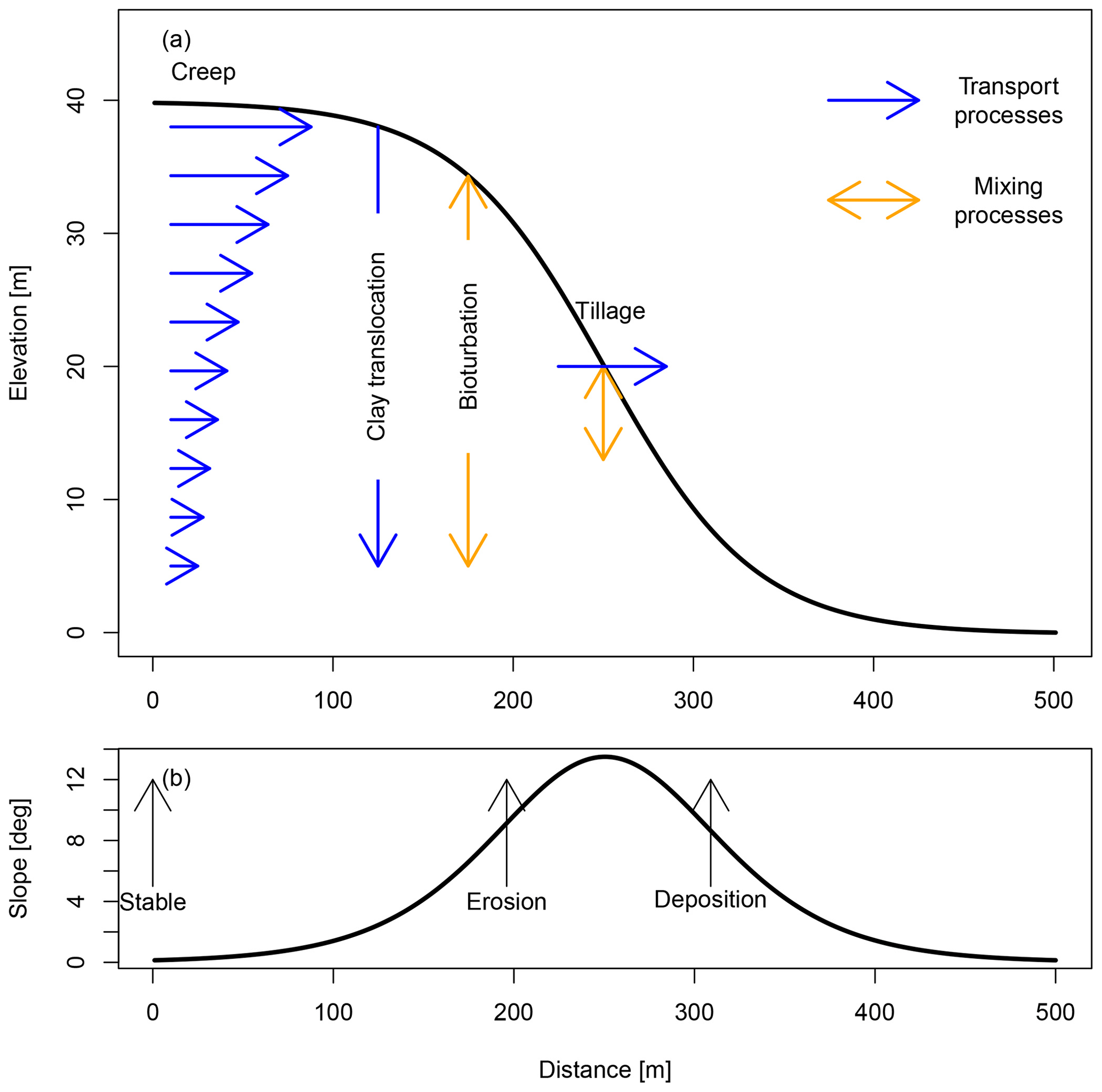
Figure 1 (a) Elevation transect of the input hillslope for the simulations with ChronoLorica. The arrows show which processes were simulated and how they affect soil particles and chronological tracers. (b) The corresponding slope transect of the input elevation. The arrows indicate the locations of the different landscape positions that are used in the data presentation.

The simulated hillslope was created to present stable, eroding and depositional positions under conditions of diffusion and has the shape of a Gaussian curve. Also, this simple hillslope facilitates visualization and explanation of the model results, which helps to understand how the model performs and what output it can create. The hillslope extends from 0 m at the ridge to 500 m at the valley bottom, with initial elevations of 40 and 0 m, respectively. Through the simulations, the elevations change under the influence of the simulated pedogenical and geomorphological processes. There are no restraints on the elevation changes. The parent material of the soils was set based on loess sediments, with 25 % sand, 60 % silt and 15 % clay. The initial soil thickness was set at 3 m, divided over 50 soil layers with a thickness of 0.05 m, with the top layer having a thickness of 5 mm, representing the OSL bleaching depth, and the lowest layer containing the remaining soil depth. The simulations started with 10 ka of natural development, where we simulated the processes of creep, bioturbation and clay translocation. This natural period was followed by 500 years of agricultural land use by introducing mixing and erosion by tillage. Figure 1 shows how the different processes affect transport and mixing of soil and chronological tracers.

The goal of this simulation was to provide insight into the functioning and applicability of the model rather than trying to reproduce measured chronologies. The selected processes, parameters, input hillslope and periods of land use are therefore a simplification of the real-world development of landscapes, but this simplification suffices to illustrate the aims of ChronoLorica. The model parameters require constraining with experimental data when the model is applied to real-world settings.

Table 1 shows the parameters used in this study. Where possible, the parameters have been taken from the literature. Where that was not possible, the parameters were estimated based on comparable studies, or they were manually set to get illustrative outcomes. This parameter selection is explained in this paragraph. The potential creep and bioturbation rate (CR_pot and BT_pot) were based on soil fluxes by various organisms, such as roots (∼ 5 kg m⁻²; Gabet et al., 2003) and earthworms (2–6 kg m⁻²; Wilkinson et al., 2009). The depth decay parameters for creep and bioturbation (dd_CR and dd_BT) were set to 5 m⁻¹, which limits transport and mixing to the upper metre of the soil. This value is consistent with the inverse of the depth scale of creep (6.7 m⁻¹) used in Anderson (2015). We used the same values for the creep and bioturbation parameters because we consider the soil creep to be a transport process caused by biogenic activity on hillslopes. The parameters for clay translocation (CT_adv and dd_CT) were set to simulate a soil profile with a Bt horizon ranging from ∼ 0.5 to 1 m, which is representative of soils in loamy environments (Van der Meij et al., 2017) and sets the clay translocation activity to the same depth range as the bioturbation process. The tillage constant C_til was set to 2 a⁻¹. This value produced a colluvial layer of max 1 m in the simulations. This thickness enabled us to clearly visualize the development of the chronological archive in the colluvium without numerical instability (higher values) or a limited colluvial thickness (lower values).

Table 1 Parameters used for the geochronometers and the pedogenical and geomorphological processes in ChronoLorica for this study. When the reference states “est”, the parameter is estimated. See the main text for the motivation of this parameter selection.

4 Results

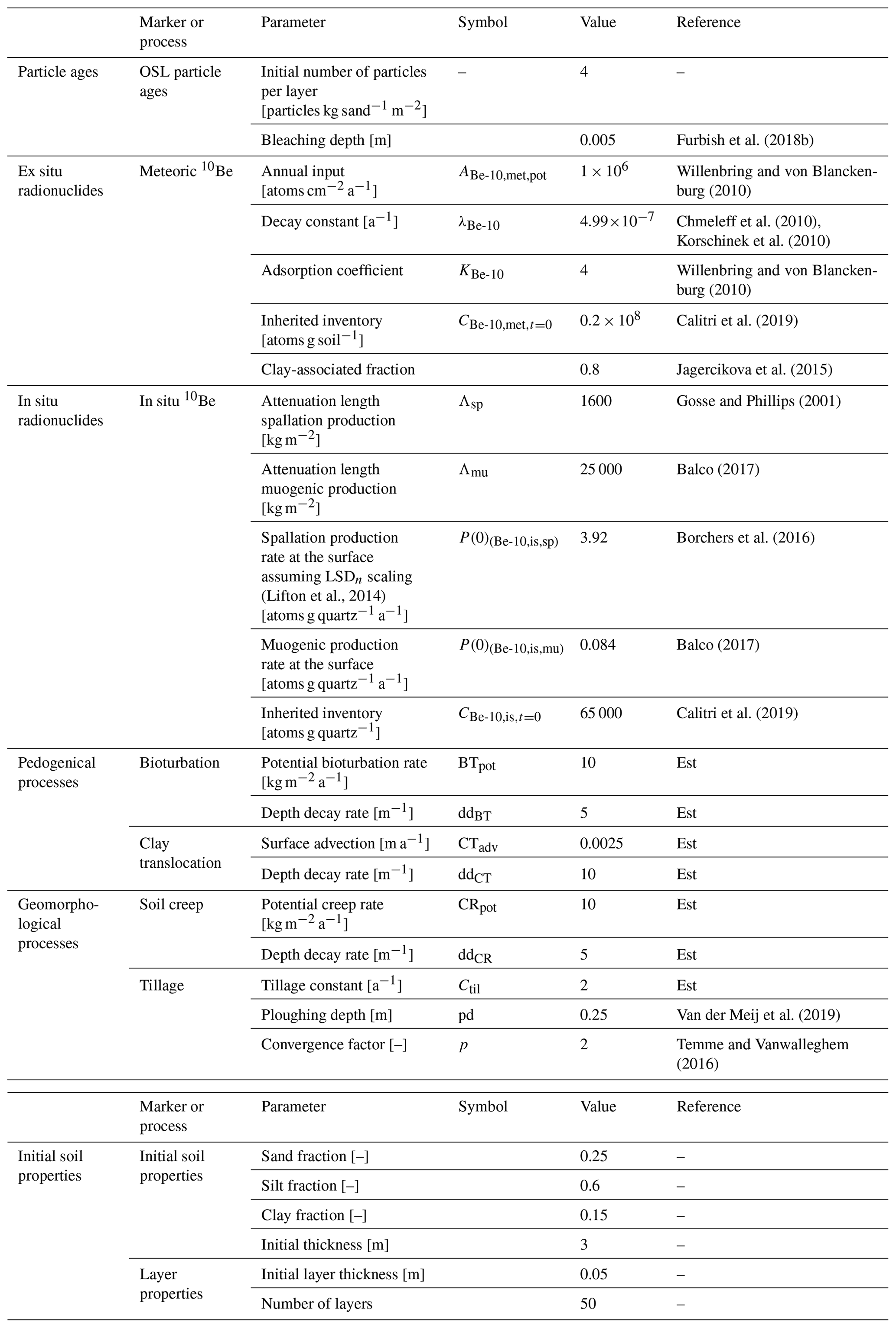
Figure 2 shows the evolution of different chronological markers for the natural phase of soil and landscape evolution. The OSL particle age–depth plot (Fig. 2a) shows an increasingly steep depth profile. At the bottom of the profile, below 1.2 m, the average OSL particle age increases equally with the simulation time. Closer to the surface, the average OSL particle age deviates increasingly from the simulation time throughout the simulations. In the top soil layer, which is completely bleached, the particles have an average age of 0 years. Over time, the depth at which the rejuvenated ages can be found increases. The wiggles in the age–depth curves are due to the limited number of particles per layer and show the stochastic behaviour of particle transport. With an increasing number of particles, the curves become smoother. Figure 2b shows the age distributions after 10 ka of simulations. In the subsurface, the majority of the particles have an age of 10 ka, equal to the simulation time, while layers closer to the surface contain an increasing number of particles with younger ages, which were mixed into the subsoil due to bioturbation. The age of these rejuvenated particles increases with depth. At a depth of 1.5 m, there are no rejuvenated particles present.

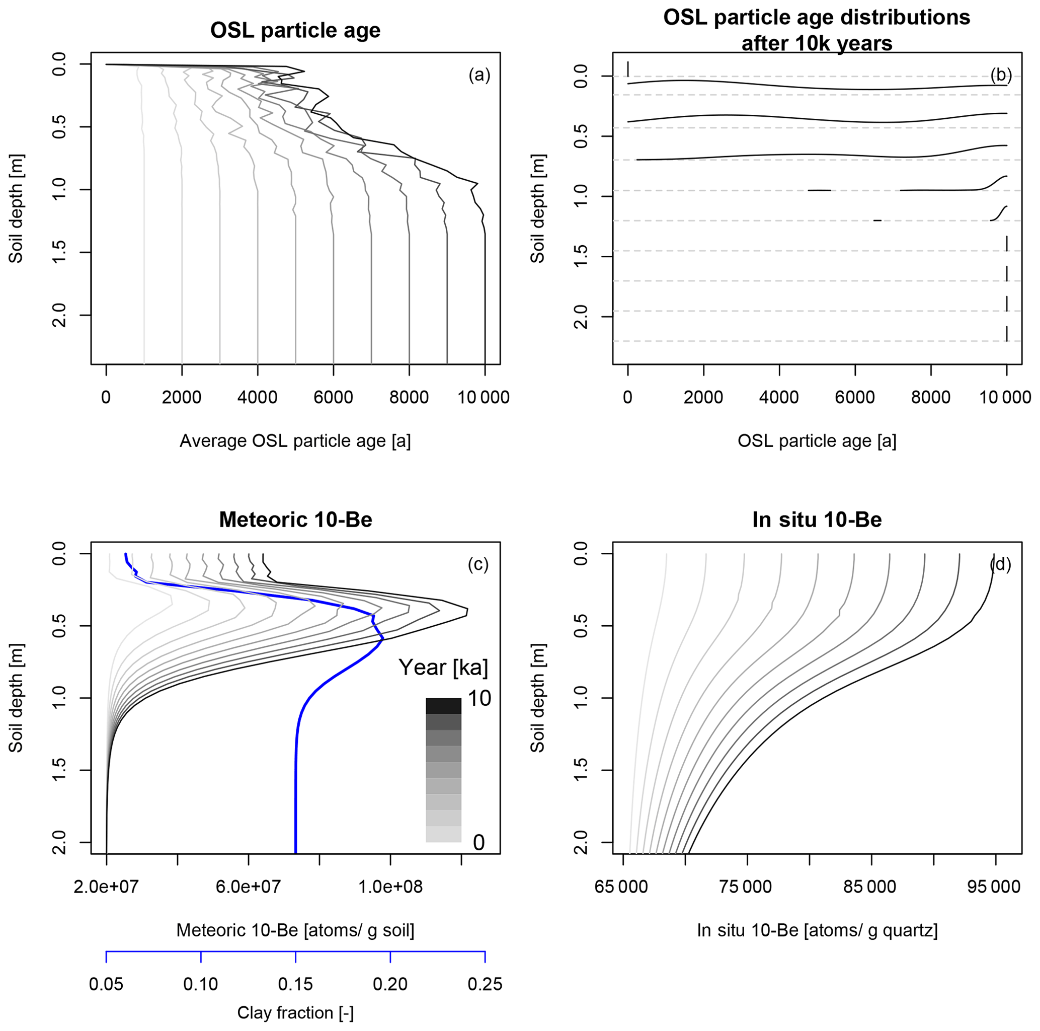
Figure 2 Evolution of chronologies at a stable position in the simulated landscape in the first 10 ka of simulations (natural phase). The shading of the lines indicates the time in the model simulations. (a) Evolution of the average OSL particle age–depth plot over time. (b) OSL age distributions of particles in a selection of soil layers after 10 ka of simulations. (c) Evolution of the meteoric ¹⁰Be–depth plot over time. The clay–depth profile at time step 10 000 is indicated in blue. (d) Evolution of the in situ ¹⁰Be–depth plot over time.

The meteoric ¹⁰Be–depth profile (Fig. 2c) develops a bulge shape. The shape of the bulge closely follows the shape of the clay–depth profile. The profiles show continuously increasing inventories over the entire profile. Below 1.5 m, the inventories have a constant value of 2×10⁷ atoms g soil⁻¹, which was the inherited inventory for meteoric ¹⁰Be.

The in situ ¹⁰Be–depth profile (Fig. 2d) also shows continuously increasing inventories over time. The lower parts of the profiles follow an exponential curve, but the upper part of the curve, above 0.75 m, deviates from that curve. Here, the inventories become more similar towards the soil surface, showing homogenization effects of bioturbation.

Figure 3 shows how the chronological markers change at different landscape positions under the influence of tillage erosion in the agricultural phase. At the relatively stable position, the elevation of the soil surface shows a small decrease of 0.10 m. In the plough layer, the OSL particle ages show a large decrease compared to the age–depth profile in the natural phase, with average OSL particle ages around 0.5 ka. Most of the particles in the plough layer have been bleached, but the unbleached particles have a disproportionate effect on the average ages. This effect is visualized in Fig. 4, which shows more detailed age information for the depositional location. Below the plough layer, there is also a reduction in the average age. The meteoric ¹⁰Be at this position shows a homogenized inventory in the plough layer (Fig. 3). The inventories are not completely homogeneous because of the unit the inventories are expressed in. Deviations in the soil mass cause small deviations in the concentrations of meteoric ¹⁰Be. When expressed in atoms per gram silt and clay, the fraction that the meteoric ¹⁰Be is associated with, the inventories are identical for every layer in the plough layer. For the in situ ¹⁰Be, expressed in atoms per gram sand, there is also a homogeneous inventory in the plough layer.

The erosion position shows a decrease in elevation of 1.04 m. This lead to a truncation of the cosmogenic nuclide depth profiles. Aside from the mixing in the plough layer, the depth profiles follow the same trend as the natural depth profiles. In the plough layer, the inventories are higher compared to the natural profile at the same depth. The age–depth profiles also show a truncation, where the subsurface depth profiles are similar. In the plough layer, the OSL particle ages are again much younger compared to in the natural setting, but they are older compared to the particles in the plough layers at the stable and deposition locations.

The deposition location has an elevation increase of 1.04 m. At this location, the effects of tillage are 2-fold. First, the chronological markers were disturbed in the plough layer, homogenizing the cosmogenic nuclides and resetting OSL particle ages, similarly to the stable position. Second, colluvial material was transported towards this location, building up a layer of colluvium, with additional cosmogenic nuclides and particles. The average OSL particle ages in the plough layer are similar to those in the stable position. In the colluvial profile below the plough layer, OSL particle ages slowly increase up to the depth where the soil has not been affected by tillage. Meteoric ¹⁰Be shows a new bulge shape developed in the colluvial profile. The in situ ¹⁰Be shows a slowly decreasing inventory in the colluvial profile towards the surface.

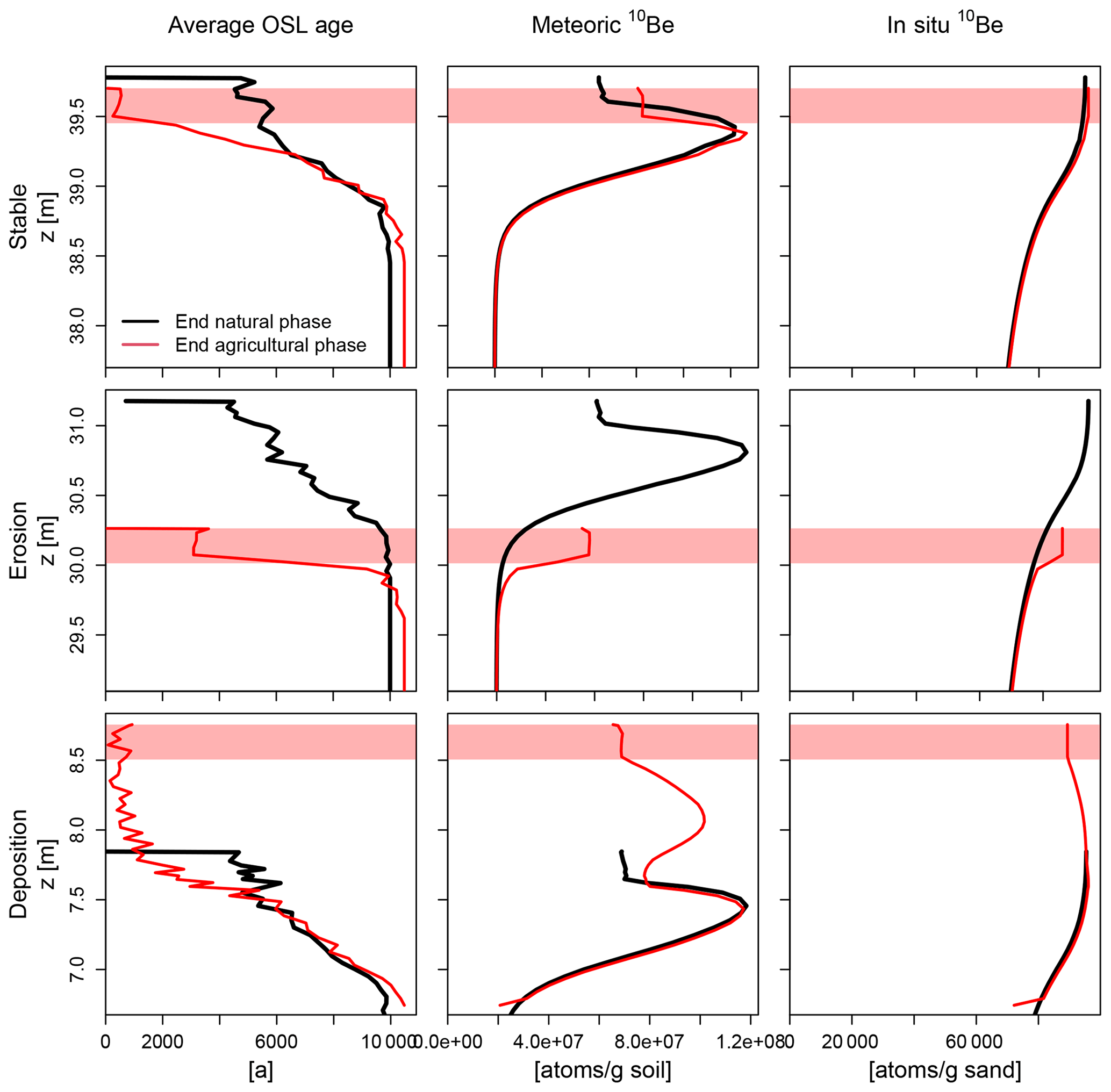
Figure 3 Changes in the simulated chronologies due to tillage erosion in three different landscape positions (for locations, see Fig. 1). The y axes show the absolute elevation of the soil layers to illustrate elevation changes due to erosion and deposition. The black lines indicate the end of the natural phase, and the red lines indicate the end of the agricultural phase. The red band indicates the depth of the plough layer at the end of the agricultural phase.

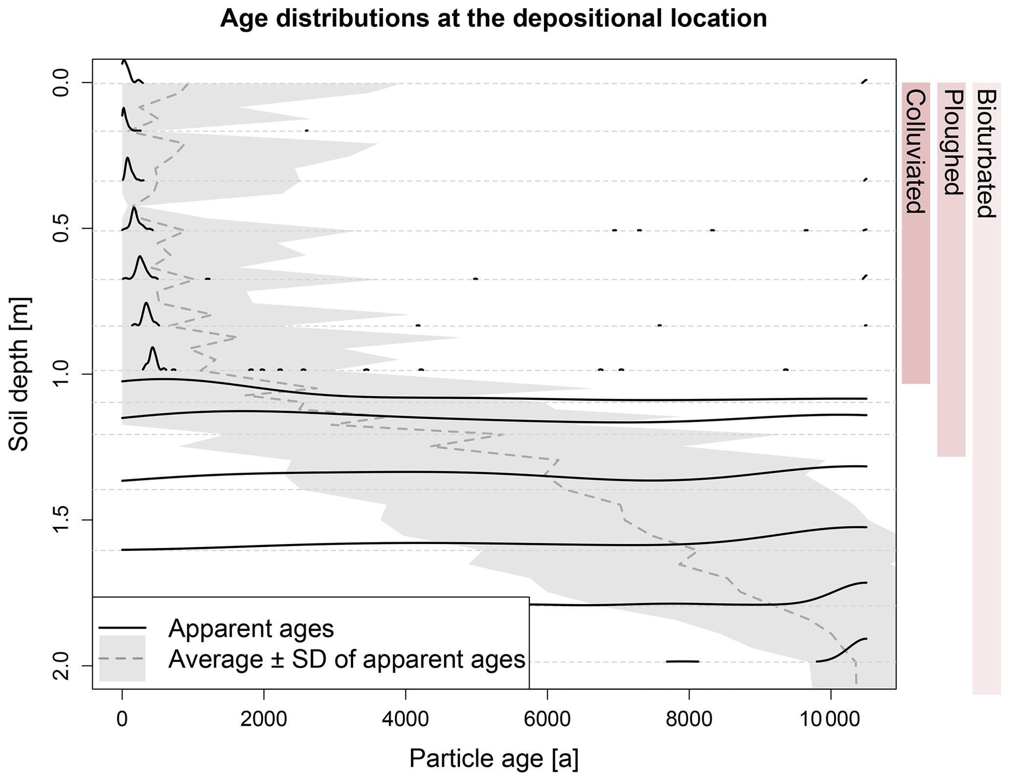
Figure 4 Detailed age information for the depositional location. Age distributions of OSL particle ages, as well as the average and standard deviation of the OSL particle ages, are provided. The columns on the right indicate over which depths different processes affected the OSL particle ages.

Figure 4 shows a detailed age–depth profile at the depositional location. Under the former soil surface, at ∼ 1 m depth, the age–depth profiles globally follow the age–depth profile created by bioturbation. There is no large rejuvenation in the top layers of this former soil, although these have also been tilled. Due to the high erosion and deposition rates as a result of tillage, only a small part of the particles in this plough layer had the opportunity to bleach before they were buried under new colluvium. The colluvial layer in the upper metre contains a high number of bleached particles but also still some unbleached particles.

Figure 5 show the development and changes in the cosmogenic nuclide inventories along the hillslope. In the natural phase, the inventories of both meteoric and in situ ¹⁰Be develop rather homogeneously and linearly along the hillslope, with only minor spatial variation (Fig. 5b and d). The inventories increase linearly with time. Both types of ¹⁰Be develop similarly, although with different magnitudes. In the agricultural phase, the elevation changes drastically due to the introduction of tillage erosion (Fig. 5a). This also affects the ¹⁰Be inventories (Fig. 5c and e). The inventories show very different dynamics and rates of change compared to a natural landscape. The changes in inventories correspond closely to the elevation changes.

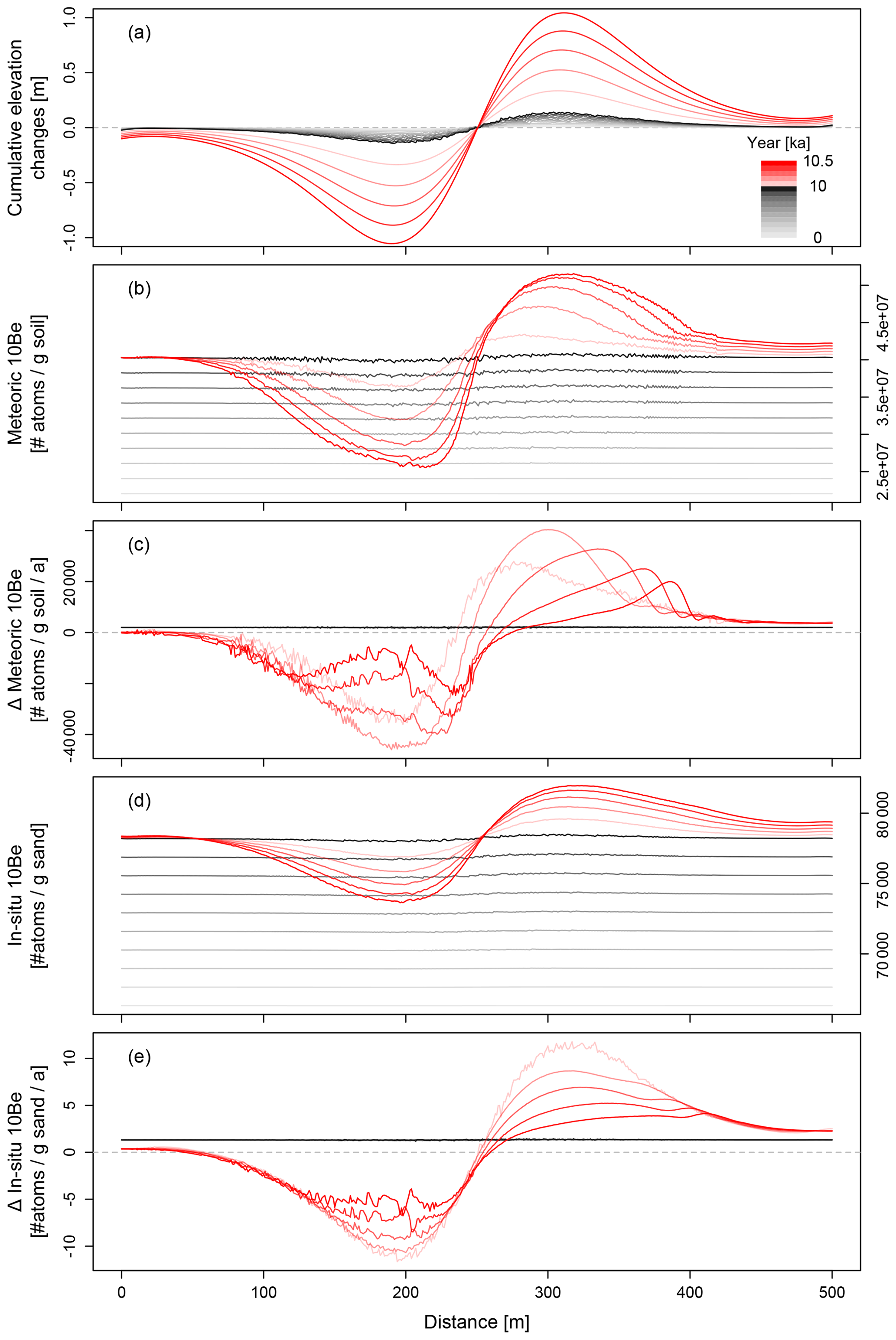
Figure 5 Changes in elevation and cosmogenic nuclide inventories along the hillslope. The cosmogenic nuclide inventories show the total inventories for each soil profile. Grey colours indicate the natural phase. Red colours indicate the agricultural phase. Time steps in between the results for the natural phase are 1000 years, and for the agricultural phase, they are 100 years. The dashed lines in (a), (c) and (e) indicate zero change. (a) Changes in elevation. (b) Changes in meteoric ¹⁰Be inventories. (c) Rate of change in meteoric ¹⁰Be inventories. (d) Changes in in situ ¹⁰Be inventories. (e) Rate of change in in situ ¹⁰Be inventories. For (c) and (e), differences in changes in the natural phase are very minor compared to in the agricultural phase and are not visible on this scale.

5 Discussion

5.1 Simulated development of chronologies

The simultaneous simulation of soil and landscape evolution and the development of chronologies can provide new insights into the processes that form and affect the chronologies. In this Section, we discuss the simulated vertical, lateral and temporal distributions of geochronometers. We compare the simulations to observed profiles and add suggestions as to how simulations with ChronoLorica can support experimental studies on soil processes.

5.1.1 Depth profiles

Depth profiles of cosmogenic nuclides and OSL particle ages help to understand the soil processes that are responsible for the development of these profiles (e.g. Graly et al., 2010; Johnson et al., 2014; Gray et al., 2020). The other way around, the simulation of these processes can help us understand which preconditions and rates are required to develop depth profiles that can be observed using field and experimental data. The simulated OSL particle age– and ¹⁰Be–depth profiles (Fig. 2) resemble observed depth profiles. For example, the bulge shape of the meteoric ¹⁰Be resembles profiles observed in French loess soils (Jagercikova et al., 2015). Also, for the bulge shape of meteoric ¹⁰Be that developed in the colluvium of the depositional profile, field analogues can be found (VAMOS profile in Calitri et al., 2019). Jagercikova et al. (2015) simulated the development of their observed profiles using an advection–diffusion equation, on which Lorica's clay translocation process is based (see Sect. 2.2). This shows how experimental data can help develop modelling tools for simulating the development of the observed profiles. When observations and simulations match well, the simulations can be expanded with additional processes or other landscape positions to understand how these extra factors influence the developments of chronological markers. For these locations, experimental approaches might not be applicable because erosion processes can disturb the chronologies and complicate their interpretation. Numerical simulations also provide the opportunity to test how different process rates and initial and boundary conditions affect the shape of the depth profiles (e.g. bulge, decline or uniform shapes; Graly et al., 2010) without the need to find suitable field analogues.

The simulations in the natural phase show characteristic depth profiles for OSL particle ages and in situ ¹⁰Be (Fig. 2), formed under bioturbation (Wilkinson and Humphreys, 2005; Johnson et al., 2014; Román-Sánchez et al., 2019a). The decreasing OSL particle ages towards the soil surface are a direct consequence of mixing by bioturbation. The rate at which bleached particles are mixed into the soil depends on the following two factors: the mixing rate and the bleaching depth. The mixing rate is an obvious factor; with more intensive mixing, particles can reach more quickly and deeply into the soil. The bleaching depth is a parameter that determines the supply of bleached particles. A larger bleaching depth supplies more bleached particles. Experimental data on bleaching depths in soils are scarce, and often numerical models are used to estimate these depths (Furbish et al., 2018b). Factors that probably affect bleaching depths in soils are soil type and texture, vegetation cover, and surface roughness affected by land use. To further improve the numerical modelling of OSL ages in soils, additional experimental data on bleaching depths are required.

Soil mixing in the upper part of soil profiles has been hypothesized and observed to affect radionuclide–depth profiles (Schaller et al., 2009; Hippe, 2017). This is also visible in our simulations (Fig. 2d), where the upper part of the in situ ¹⁰Be deviates from the expected exponential curve. The topsoil does not show a uniform concentration of in situ ¹⁰Be, as suggested in Hippe (2017), because the soil is not completely mixed, as happens with tillage, and because mixing rates decrease with distance from the surface. This mixing pattern is typical for many natural soils (Gray et al., 2020) and can be used to quantify mixing rates (Wilkinson and Humphreys, 2005). Comparison of observations and model results using various ways and rates of simulating bioturbation will provide new insights into the applicability of cosmogenic nuclides for soil-mixing studies. However, as Hippe (2017) remarks, there is still a lack of field data for supporting such studies.

Tillage is a much more intensive mixing process than bioturbation, creating uniform cosmogenic nuclide inventories and age distributions in the plough layer, as suggested by Hippe (2017). The homogenization and bleaching caused by tillage on the entire hillslope affects how the age–depth profiles develop at different landscape positions. Erosion by tillage excavates lower cosmogenic nuclide inventories or unbleached particles from the subsoil into the plough layer, which are consequently transported and affect these properties elsewhere. There is also a reverse effect of the mixing, namely that the concentration of bleached particles increases at the bottom of the plough layer. These particles can then be transported into the subsoil by bioturbation, leading to younger average ages below the plough layer in the stable position (Fig. 3). The particles in the colluvium are well bleached, with only a few unbleached particles (Fig. 4). This contrasts with hypotheses of partial bleaching in colluvial soils (Fuchs and Lang, 2009). The intensive mixing by tillage causes bleaching of particles already at their erosional locations. These pre-bleached particles are consequently transported and deposited, creating a well-bleached colluvium. The average OSL particle ages do not match with the modes of the age distributions (Fig. 4) due to the presence of some older or unbleached grains. A minimum-age model might be necessary to extract the required age information from the model results, similarly to partially bleached sediments from the field (Arnold et al., 2009; Cunningham and Wallinga, 2012; Van der Meij et al., 2019). Age corrections might be required to account for the effects of post-depositional mixing on the chronology (Van der Meij et al., 2019).

5.1.2 Lateral redistribution patterns and rates

Next to soil development at a pedon scale, simulations with ChronoLorica also show how soils, landscapes and chronologies can evolve on a hillslope to landscape scale. This will help to understand where and how chronologies can form. This can assist in sampling-site selection, the testing of hypotheses for landscape evolution (Crusius and Kenna, 2007) or the calculation of erosion and deposition rates through model calibration (Temme et al., 2017).

The effect of soil creep in the natural phase is limited with our parameter set, with elevation changes ranging from −0.12 to +0.11 m in 10 ka, which corresponds to rates of $-\mathrm{12}\times {\mathrm{10}}^{-\mathrm{3}}$ to $+\mathrm{11}\times {\mathrm{10}}^{-\mathrm{3}}$ mm a⁻¹. Creep rates reported for temperate and tropical environments range from 0.5–10 mm a⁻¹ (Saunders and Young, 1983), although the slopes of these measured rates (0 to >25^∘) are, in general, steeper than the ones in the simulations (average 4.5^∘, max 14^∘; Fig. 1). Nonetheless, the measured rates are 2 to 3 orders of magnitude higher than the simulated rates. The difference in rates might be explained by Eq. (1), where the potential creep rate is multiplied with the slope gradient, which reduces the local rate substantially on our gently sloping landscape. Simulated tillage rates range from −2 to +2 mm a⁻¹ and fall in the range of reported average agricultural erosion rates, although these reported rates show a very large spread (∼ 0.1–10 mm a⁻¹ for 95 % of the reported values; Montgomery, 2007). To further understand these geomorphological processes in real-world settings, calibration with field data is required. This becomes possible when setting up model studies for specific landscapes where creep and/or tillage rates have been empirically determined.

The simulated chronologies show which geochronological methods are applicable for different landscape positions and over different timescales. For the cosmogenic nuclides, comparison between stable, eroded and deposition locations provides information on erosion and deposition rates (Fig. 3; Phillips, 2000; Willenbring and von Blanckenburg, 2010; Calitri et al., 2019). At the deposition location, the built-up colluvium contains a stratigraphic record of OSL particle ages (Fig. 4) that can be used for determining deposition rates using conventional OSL measurements, although age corrections might be necessary to correct for post-depositional mixing processes (Van der Meij et al., 2019). At the stable or eroded position, there is no chronology that can be measured to determine erosion rates. However, as Fig. 3 shows, the truncation (i.e. decapitation of depth profiles) of the OSL particle age–depth profile is similar to the truncation of the ¹⁰Be–depth profiles. This suggests that quantitative erosion rates can be determined by the level of truncation of bioturbation age–depth profiles, similarly to truncation of radionuclide profiles (Arata et al., 2016a, b) or soil horizon profiles (Van der Meij et al., 2017).

ChronoLorica can be a valuable tool for evaluating and comparing different geochronometers. The simulations form a controlled experiment, with known rates of landscape change. The simulated changes in geochronometers can be used to evaluate their spatial and temporal resolution, to compare different geochronometers, and to test analytical methods for determining erosion and deposition rates.

5.2 Limitations of ChronoLorica

ChronoLorica has several advantages over other numerical methods for simulating chronological development. These are its applicability for both steady-state and transient landscapes, the possibility to simulate multiple geochronometers, and the possibility to simulate various processes, including secondary processes such as post-depositional mixing. The previous sections have highlighted and illustrated these advantages. Here, we discuss model limitations.

5.2.1 Model uncertainties

Uncertainties in ChronoLorica mirror those in most soil–landscape evolution models. These relate to process formulations, initial and boundary conditions, and data limitations (Minasny et al., 2015). Lorica and ChronoLorica are developed mainly for Holocene and Anthropocene soil and landscape development, where changes in soils occur at similar rates as changes in the landscape. The architecture and process descriptions of the model were adjusted to these long timescales, with simplified process descriptions. The model will be difficult to apply to shorter timescales (sub-annual to several years) because, over these timescales, changes in soils, sediments and chronologies occur episodically. This behaviour is not captured in the simplified process descriptions, which simulate gradual changes over time. The model can be applied over longer timescales than the Holocene, but additional development might be required to include processes acting on these timescales and their effect on chronologies, such as weathering processes. The architecture of ChronoLorica lends itself well to these adjustments, but extra care should be given to the increased runtime and calculation demands of the model (see next Section).

All SLEMs face uncertainties coming from uncertain initial and boundary conditions. Over the simulated timescales, it is usually difficult, if not impossible, to make accurate reconstructions of the shape of the initial landscape, the properties of the parent material, and climatic and anthropogenic changes over time (Minasny et al., 2015). A way to reduce or bypass these uncertainties is by performing simulations on hypothetical landscapes, as is done in this paper. This gives insights into how soils, landscapes and chronologies might react to different processes, rates and changes in boundary conditions and can help to better understand the development of real-world landscapes. However, when these real-world landscapes are the topic of interest, the simulations are still dependent on local or regional reconstructions of initial and boundary conditions. These reconstructions are often made using different chronological methods, such as pollen analysis and ¹⁴C dates for climate and vegetation reconstruction (Mauri et al., 2015) or OSL and other dating methods for regional land use history and landscape change (e.g. Kappler et al., 2018, 2019; Pierik et al., 2018). These reconstructions serve as input for SLEMs, but, interestingly, SLEMs such as ChronoLorica can also be used to better understand the chronologies that have been used for developing these reconstructions. It is attractive to imagine this as an iterative process, where initial understanding of the observed chronologies is adapted and refined using model simulations. This, in turn, leads to different initial and boundary conditions and thus to adapted model outputs, as envisioned in Temme et al. (2011).

5.2.2 Runtime and memory constraints

The runtime of the model, i.e. the time it takes to finish a simulation, depends on the vertical and temporal discretization of the model scenario: raster dimensions and cell size, number of soil layers, and the number of time steps in the model. The runtime increases supralinearly with the dimensions of the soil landscape. For instance, for bioturbation, the number of calculations increases exponentially with the number of soil layers because there is an exchange between each soil layer and all other layers. The simulations for this paper, with a raster of 1 by 501 cells, 25 soil layers and 10 500 simulation years, took nearly 20 hours on an average (year 2022) laptop with an Intel Core i7 processor with 6 cores, a 2.7 GHz clock speed and 16 Gb of RAM.

The spatial and temporal dimensions of a simulation thus need to be chosen with care to limit the runtime of a simulation. For two-dimensional landscapes, the cell size of the input raster can be increased to reduce the number of raster cells. The thickness of the soil layers can also be adjusted. ChronoLorica provides the option of varying soil layer thickness, where layers closer to the surface are thinner than subsurface layers. This provides more detail in the zone where most variation is expected. When choosing the number and thickness of soil layers, the vertical range of different processes should also be considered. For example, when the plough depth is set to 25 cm, the layer thickness should ideally be much smaller to prevent the plough layer from mixing layers that are partially located in the plough depth. The layer thickness of 5 cm in our simulations is relatively large but was chosen to limit the calculation time.

From the geochronological module, runtime is substantially increased by the particle tracing. With each movement of sediments, either laterally by geomorphological processes or vertically by soil processes, there is a probability that the particles in the source layers will move as well. For each individual particle, the model probabilistically assesses whether it moves together with the sediment. This requires a lot of extra calculation steps. In comparison, radionuclide inventories require only one extra calculation step, as a fraction of the inventories is moved between the layers.

The choice of the number of particles per layer should depend on the following three factors: the spatial and temporal discretization of the model, the simulated processes, and the sand content of each layer. For a one-dimensional simulation of soil profile development, for example by bioturbation, many more particles can be simulated in the same calculation time as a full three-dimensional landscape. Bioturbation requires a lot of calculation time, especially when the OSL particle age module is activated. When simulating three-dimensional landscapes, it is wise to consider whether bioturbation has a large effect on the chronologies compared to the other processes. If not, the exclusion of the bioturbation simulation can be considered. The final consideration is the sand content of each layer, as the particles are associated with sand fraction. It is important to choose the number of particles in a way that the bleaching layer has at least one or two particles present. Otherwise, there is a chance that particles will not be bleached in the model run or that the distribution of OSL particle ages will not provide usable information. A way to estimate the number of particles in the bleaching layer is by multiplying the bleaching depth with the cell size, an average bulk density (e.g. 1500 kg m⁻³) and the sand fraction. This gives the sand content in the bleached layer, which can be used to estimate the initial number of particles per kilogram of sand. In this paper, this results in 0.005 ⋅ 1 ⋅ 1 ⋅ 1500 ⋅ 0.25 = 1.9 kg sand. With four particles per kilogram of sand, this results in approximately eight particles in the bleached layer.

Increasing spatial and temporal dimensions also influences the memory requirements of the model and the size of the output data. The output of the simulations for this paper, on a one-dimensional hillslope, is 6 GB in size, with outputs for every 100 simulation years. A total of 86 % of these data are output files containing the OSL particle age information. Constraining the spatial and temporal dimensions of the simulations will also help to constrain the memory requirements for the simulations and will help speed up the analysis of the model output.

We propose the following workflow when applying the model. First, run the simulations without the geochronological module to get an understanding of the spatial and temporal variations in soil and landscape properties. Based on that, the spatial discretization can be chosen. Second, determine the number of particles per kilogram of sand using the guidelines described above. Lastly, run the model with the geochronological module to get the required age information.

5.3 ChronoLorica for other pedogenical, geomorphological or geological applications

The current version of ChronoLorica was developed with agricultural landscapes in mind because these transient landscapes show the highest rates of landscape change, which are difficult to measure with conventional methods (Calitri et al., 2019). ChronoLorica can, in theory, be adapted for other landscapes, settings and processes. In this section, we mention several possible applications and the adaptations to the model they would require in order to inspire further integration of soil–landscape evolution models and geochronometers.

5.3.1 Calibration of bioturbation processes and rates

Bioturbation, the process where soil biota mixes the soil, affects the redistribution of geochronometers as well (Wilkinson and Humphreys, 2005). By confronting ChronoLorica with experimental data, the bioturbation rate and depth decay rate can be calibrated. ChronoLorica can also be used to test various formulations of the bioturbation process. Currently, we simulate bioturbation as a process where the entire profile is prone to mixing, with exponentially decreasing rates further from the surface. This process resembles soil mixing by earthworms. Other process descriptions, such as upward transport of particles, for example by termites (Kristensen et al., 2015), or instantaneous mixing of a soil body by tree uprooting (Šamonil et al., 2015) can be implemented in the model, and its effect on chronologies can be simulated. This can also include other depth functions. This flexibility facilitates hypothesis testing for determining which bioturbation process might have been responsible for an observed depth profile.

5.3.2 Spatial and temporal variations in dose rate

With OSL dating, the soil or sediment ages are determined by dividing the palaeodose of a sample of soil or sediment particle(s) by the dose rate. The dose rate is the sum of all ionizing radiation coming from the surrounding soil, sediments and cosmic rays. The dose rate is partially attenuated by different particle sizes, water and organic matter (Madsen et al., 2005; Durcan et al., 2015). In most experimental studies, the dose rate that is measured at the sampling location is taken as the representative for all particles taken from that position. However, in the case of mixing processes in the soil, particles travel through the soil profile. During their soil passage, these particles can receive different dose rates at different depths due to variations in ionizing radiation from the surrounding soil and cosmic rays (Prescott and Hutton, 1994) and also variations in moisture and organic matter content. Dose rates can also change over time due to changes in disequilibria in radionuclide decay chains (Olley et al., 1996), changes in soil mineralogy by weathering, clay translocation and erosion, and/or deposition. Dose rates can thus be variable in space and time.

Although we currently do not track dose rates or palaeodoses of particles in ChronoLorica, the model simulates soil properties that can be used to estimate spatially and temporally varying dose rates and attenuation and consequently assess how changes in dose rates affect particle ages. These soil properties are soil depth, organic matter content and clay content, which can be associated with some radionuclides (Heimsath et al., 2002). Soil moisture fluctuations and the attenuation effects are still difficult to predict with SLEMs (Van der Meij et al., 2018). With a sensitivity analysis, the model can help to determine whether spatiotemporal changes in dose rate can have a significant effect on OSL particle ages.

5.3.3 Landscape evolution modelling on soil-mantled hillslopes

A traditional application of landscape evolution models (LEMs) is to understand how soil-mantled hillslopes evolve. Over geological timescales, LEMs assume that there is a balance between soil production and soil erosion, either by water or by diffusive processes (Tucker and Hancock, 2010). Cosmogenic nuclides are a common method for studying this landscape development as well by calculating spatially varying or catchment-averaged erosion rates (Bierman and Steig, 1996; Granger et al., 1996). Most LEMs consider soils to be a mobile part of the hillslope and do not subdivide soils into multiple layers or simulate vertical transport among layers. This complicates the comparison of measured cosmogenic-nuclide–depth profiles with simulations. ChronoLorica can support these studies by simulating the cosmogenic-nuclide–depth profiles or OSL age profiles (Fig. 3) that can be compared to field measurements.

For these studies, soil processes are of minor importance, and focus can be placed on the geomorphological processes. Required adjustments to the model code include the development of a geochronological module for the bedrock-weathering process. Special care should be given to how cosmogenic nuclides are distributed initially in soils and bedrock and how weathering changes the bulk density and cosmogenic nuclide inventory upon the conversion of bedrock into soil.

5.3.4 Particle size selectivity in mixing and transport processes

ChronoLorica considers the following different grain sizes: coarse, sand, silt, clay and fine clay. Grain size controls the uptake and deposition by water or the rate of physical and chemical weathering. Other soil processes in Lorica, such as bioturbation, are currently grain size independent, although there is evidence that bioturbation can also be grain size dependent (Dashtgard et al., 2008). Empirical studies measuring geochronometers associated with different grain sizes can help the formulation of a grain-size-dependent soil-mixing module for ChronoLorica, which in turn can help to determine mixing rates for different particle sizes and to improve the simulation of age distributions. With small adjustments, ChronoLorica can consider a larger range of particle sizes, providing more detail in the simulated processes.

5.3.5 Soil weathering effects on cosmogenic nuclide distributions

Weathering is the breakdown of coarser particles into smaller particles. This can be due to physical processes, such as freeze–thaw cycles, or due to chemical dissolution processes. Chemical weathering can lead to quartz enrichment by removing other minerals. This can overestimate in situ cosmogenic nuclide production (Riebe et al., 2001), change cosmogenic nuclide inventories from weathering bedrock into finer soil fractions (Ott et al., 2022) or even promote the bleeding of in situ ¹⁰Be into meteoric ¹⁰Be pools. With the addition of a chronological module to the different weathering processes in ChronoLorica, the effects of weathering on cosmogenic nuclide distributions can be quantified.

6 Conclusions

ChronoLorica is a coupling between the soil–landscape evolution model Lorica and a geochronological module, which traces various geochronometers throughout the simulations of soil and landscape development. The model simulates realistic spatial and temporal patterns of the geochronometers under both natural and agricultural land use conditions. It simulates these patterns over large spatial and temporal extents with high resolution and therefore provides rich possibilities for data-based calibration. By combining different geochronometers, the model can be applied in both steady-state and transient landscapes, where quickly changing boundary conditions, such as land management intensification and climate change, increase rates of landscape change and create complex geo-archives. The flexible framework of ChronoLorica can be expanded with other geochronometers and processes, which facilitates its deployment in different pedogenical, geomorphological and geological applications.