Anomalous fading correction in luminescence dating – a mathematical reappraisal

Anomalous fading is a power law decay of trapped charge over time that is commonly observed in wide-bandgap semiconductors, leading to age underestimation in luminescence dating if unaccounted for. In this paper, we reappraise the mathematical foundations of luminescence signal correction and introduce two new closed-form analytical expressions for the two most commonly used age correction models, namely that of Huntley and Lamothe (2001), and that of Kars et al. (2008). These expressions are amenable to straightforward uncertainty propagation, matching results from Monte-Carlo simulations at a fraction of the calculation cost. Additionally, we explore unorthodox combinations of signal fading and growth pathways, by coupling fading models to signal growth obeying general order kinetics, as well as the one-trap one-recombination center model.

1 Introduction

Anomalous fading is, to date, an undisputedly convoluted subdiscipline in luminescence dating that creates equal discomfort for students and professors alike. Upon a closer and critical look, much of the confusion around the subject can be traced back to the insecure and sometimes misleading mathematical footing of its seminal papers, which has been tiptoed around by a wealth of recirculated measurement protocols, analysis spreadsheets, and data reduction packages, all of which patch the theoretical ambiguities and inconsistencies in numerically divergent ways. While the latter reflects the subject's relevance and active public engagement, the obfuscated math has nevertheless nudged practitioners towards strong conformity to “best practices”, which are rarely challenged but are increasingly difficult to justify. While we acknowledge the fundamental value of the various contributions on fading quantification and correction, these contributions unfortunately have a number of shortcomings, which generally fall into one of the following categories:

1. Erroneous mathematical statements and substandard formulations. Wintle (1973) stated that her observations of anomalous luminescence signal loss (Fig. 1a) did not exhibit simple time dependence, although these data do in fact exhibit logarithmic decay (inset Fig. 1a). Wintle's (1973) erroneous statement overlooked more than a century of phosphorescence research demonstrating the ubiquity of power-law decay behavior in general (Becquerel, 1867; Randall and Wilkins, 1945; Medlin, 1961), and tunnelling-driven kinetic models in particular (Hoogenstraaten, 1958; Thomas et al., 1965; Riehl, 1970). With respect to formula conventions, the decay formulas of Visocekas (1976, 1985), Aitken (1985), and Huntley and Lamothe (2001) regrettably normalized the use of hardcoded percentage units, in disregard of the standard unit-independent formulation of physical laws (Maxwell, 1873; BIPM, 1970).

2. Misleading derivations. Visocekas (1976) made the first quantitative reinterpretation of Wintle's (1973) data (inset in Fig. 1a), however, his definition of the logarithmic decay constant (Visocekas, 1985) is at odds with its subsequent derivation, where the integration resulted in potentially negative values and consequently an unphysical model (continuous lines in Fig. 1b). As we show in Sect. 2, a self-consistent integration leads to more meaningful results (dashed lines in Fig. 1b; see Sect. 3), precluding negative concentrations and foreshadowing the model of Huntley (2006). Similarly, Lamothe et al. (2003) derived a “new equation” extending the Huntley and Lamothe (2001) correction beyond the linear part of the dose response curve. In Sect. 3.2 we show that this equation is merely a reparametrized, single-iteration restatement of Huntley and Lamothe (2001) – a tautology, not a new model. The older ages it returns owe nothing to the equation, nor to fading itself: instead, they arise from an implicit inversion of nonlinear dose response, formalized only later by Wallinga et al. (2007).

3. Algorithmic opacity. The age correction formula of Huntley and Lamothe (2001, Eq. A5) lacks the rescaling of κ, which whilst described in the text is omitted from their arithmetic. As trivial as it may be (see Sect. 2), the rescaling of a g-value from one reference time t₁ to another t₂, via $g_{\mathrm{2}}={\left[g_{\mathrm{1}}^{-\mathrm{1}}-{\log }_{\mathrm{10}}\left(t_{\mathrm{2}}/t_{\mathrm{1}}\right)\right]}^{-\mathrm{1}}$ is not reported in Huntley and Lamothe (2001), nor derived in any later publication. The first verifiable appearance of this formula is in published code (Kreutzer, 2017), further citing a private communication – the hallmark of grey literature underpinning an ambiguous primary source. Our confidence in restating Huntley and Lamothe's formula in Sect. 3.1 arises from our successful reverse engineering of their numerical examples. Similarly, Kars et al. (2008) only provided a bare rate equation for their now popular model, leaving it up to the reader to figure out how to combine it with the spatial distribution of electron-hole separation distances, even though a semi-analytical solution is rather straightforward (Fig. 1c).

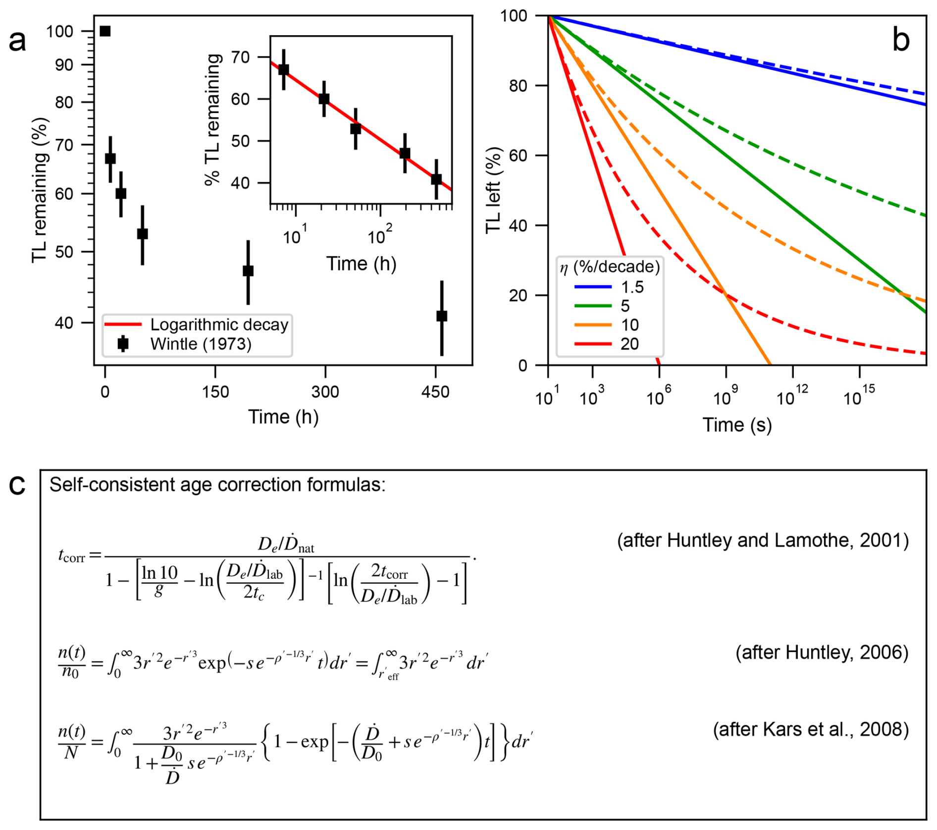
Figure 1 Characteristic problems with anomalous fading literature. (a) Erroneous statements: “the shape of the decay curve does not […] conform to any simple time dependence” (Wintle, 1973); inset: same data on a linear signal vs. logarithmic time axes, exhibiting a simple logarithmic decay at a ∼ 29 % fading rate (reference time of 2 d). (b) Erroneous derivation: negative concentrations in the model of Visocekas (1985) are inevitable (continuous lines) but can be mitigated via a more informed integration (dashed lines, see text). (c) Missing formulas from the literature: three examples of seminal formulas, whose building blocks are scattered across their corresponding papers but never brought together in a meaningful manner. The parameters are $\dot{D}$ for dose rate (with subscripts “nat” and “lab” corresponding to natural and laboratory, respectively), D_e and D₀ for equivalent and characteristic dose (respectively), t for time and T_corr for corrected age, n for the trapped electrons concentration evolving from initial n₀ to saturation N, g for the fading rate (g-value, unitless) for a reference time t_c, ρ^′ for rescaled g-value assuming escape frequency s, r^′ a dimensionless electron-hole separation distance.

The compound effect of the problems only partially listed above and illustrated in Fig. 1, has been chronic and additive: (1) erroneous statements and definitions curb the practitioners' understanding and stall further progress, sometimes for decades; (2) the few and far between mathematical derivations are taken for granted rather than scrutinized as steps towards better formulations; (3) the algorithmic opacity leads to divergent practical implementations, while still all referring to the method as one and the same (see Sect. 3.2 for an example). Our current contribution is written out of deep respect for all the fields' trailblazers, but recognizes that without a major mathematical housekeeping effort, progress will be challenging. We therefore proceed to give the shortest possible mathematical reappraisal of anomalous fading, followed by its verification, and finally some unforeseen and unprecedented variations on this rather old theme.

2 Exponential, logarithmic, and power-law decay

To define radioactive decay, Rutherford (1900) designated λ as the proportionality constant between concentration n and its decay rate with time $\mathrm{d}n/\mathrm{d}t$. Rearranging for λ and keeping its sign convention, we can express the decay constant as:

$$\begin{array}{}\text{(1)}& \mathit{\lambda }=-{\displaystyle \frac{\mathrm{d}n/n}{\mathrm{d}t}}.\end{array}$$

where the right-hand side corresponds to fractional loss of concentration ($-\mathrm{d}n/n$) per unit time (dt). Separation of variables and integration leads to the familiar $n\left(t\right)/n_{\mathrm{0}}=\exp (-\mathit{\lambda }t)$, in which $t={\mathit{\lambda }}^{-\mathrm{1}}$ is the amount of time it takes concentration to e-fold (i.e. reduce to $\mathrm{1}/e$ of its initial value at t=0).

Visocekas (1976, 1985) both coined the term “logarithmic decay”, and defined the associated decay constant as “the slope of the TL light sum vs. ln t”, which following our nomenclature of n for concentration (= the light sum in TL), and utilizing the identity $d\left(\ln t\right)=\mathrm{d}t/t$, should be formally expressed as:

$$\begin{array}{}\text{(2)}& \mathit{\eta }=-{\displaystyle \frac{\mathrm{d}n}{\mathrm{d}t/t}}.\end{array}$$

which must bear units of concentration. Nevertheless, just a few lines following his definition, Visocekas (1985) arbitrarily rescaled the denominator from dlnt to dlog₁₀t (invoking the familiar “per decade of time”), and further assigned units of [%] to η's numerator, thus disclosing a miscommunicated normalization of η by some arbitrary concentration n_c. It is the proliferation of these faux units in the literature (“% per decade”), and their illegitimate hardcoding into all familiar formulas (cf. Visocekas, 1985; Huntley and Lamothe, 2001; cf. Slater et al., 2001), that leaves little doubt that Visocekas' “logarithmic decay” (Eq. 2) should be viewed as a special case of the more general power-law decay:

$$\begin{array}{}\text{(3)}& \mathit{\kappa }=-{\displaystyle \frac{\mathrm{d}n/n}{\mathrm{d}t/t}}.\end{array}$$

where fractional concentration loss $-\mathrm{d}n/n$ is scaled by fractional (rather than absolute, cf. Eq. 1) progression in time d$t/t$. Note that our Eq. (3) is a classic example of “dimensionless sensitivity” (Beck, 1970; Smith, 1994; Smertenko, 2020), defined as the “fractional change in [a] calculated observable divided by the corresponding fractional change in the [corresponding] parameter of the model” (Smith, 1994). Also note that Eq. (3) is fully consistent with the definition of κ by Huntley and Lamothe (2001), Eq. (3) being merely the infinitesimal generalization of their finite $\mathit{\kappa }=-(\mathrm{\Delta }n/n_{\mathrm{c}})/(\mathrm{\Delta }t/t_{\mathrm{c}})$. Below we show that it is specifically Eq. (3), that all familiar results can be easily derived from. Visocekas' (1985) own seminal decay formula (straight lines in Fig. 1a–b):

$$\begin{array}{}\text{(4)}& {\displaystyle \frac{n\left(t\right)}{n_{\mathrm{c}}}}=\mathrm{1}-\mathit{\kappa }\ln \left({\displaystyle \frac{t}{t_{\mathrm{c}}}}\right)\end{array}$$

may be understood as integration of Eq. (3) subject to a fixed scaling concentration, namely $\int \mathrm{d}n/n_{\mathrm{c}}=-\int \mathit{\kappa }\mathrm{d}t/t$ (cf. Eq. 2) with $n_{\mathrm{c}}=n\left(t_{\mathrm{c}}\right)=$ const as the boundary condition. Serving as the starting point for the age correction of Huntley and Lamothe (2001), Eq. (4) is however unphysical, since n must inevitably, sooner or later, plunge into negative concentrations. Visocekas (1985) dedicated half of his 1985 paper's arithmetic (Sect. 2.6 in Visocekas, 1985) trying to mitigate said effect yet to no avail (one must drop the second term of his Eq. (7) to reproduce F in his Fig. 3). To avoid the occurrence of negative concentrations, Eq. (3) must be integrated as written, with no fixed scaling, to obtain:

$$\begin{array}{}\text{(5)}& {\displaystyle \frac{n\left(t\right)}{n_{\mathrm{c}}}}=\exp \left[-\mathit{\kappa }\ln \left({\displaystyle \frac{t}{t_{\mathrm{c}}}}\right)\right]\end{array}$$

Contrary to the heuristic Eq. (4), Eq. (5) is a physical model, where concentration remains positive n>0 at all times (for a demonstration of its successful application, see Sect. 4). Note that the more familiar Eq. (4) may be considered as a special case of Eq. (5) in its linear region, where $\exp \left(-x\right)\approx \mathrm{1}-x$. For typical laboratory conditions, the curvature of Eq. (5) is unnoticeable: consider the dashed green curve in Fig. 1b (g=5 %), which could easily be mistaken for a logarithmic decay (Eq. 2) over 6–7 orders of magnitude of time. Let us reiterate, that κ in Eqs. (3)–(5) is just a unitless number, whose arbitrary rescaling into a g-value (defined as g=κln10, corresponding to the fractional loss for a tenfold increase of time, and bearing the faux units of “% per decade”), might have led to confusion. Readers familiar with the inseparable “$\mathit{\eta }/\mathrm{100}$” or “$g/\mathrm{100}$” from the seminal papers, will be disappointed to find that our present treatise does aim to comply with core metrological principles (BIPM, 1970), and therefore drops the familiar “100” factor as well as the pseudo “per decade” units for good. Indeed, κ is just a unitless number, and so is the commonly reported g value, or any other imaginable normalization of κ: as a thought experiment, consider h=κln2 reported in “ppm per octave (i.e. doubling) of time”. No matter the normalization, all such values will be just unitless fractions, proportional to the dimensionless sensitivity in Eq. (3) via a constant.

If either κ (or g) are obtained by fitting Eq. (4), one must report the vicinity of t around which it has been derived. This is known as the “reference time” t_c, which is conventionally set to 2 d (reflecting the typical timescale of a laboratory experiment). It is noteworthy that few laboratories report their t_c duration, and even fewer manage to do it correctly; for example, rather than being 2 d g-values as stated, the values reported in Thiel et al. (2015) are demonstrably scaled to the shortest fading measurement duration (in the vicinity of ∼ 10 min), and thus underestimate the actual 2 d g-values (by a few percent relative, and ∼ 0.1 % absolute). Nevertheless, t_c is a crucial parameter for validating one's data analysis. Due to the logarithm in Eq. (4), the decay constant (whether κ or g) is only weakly dependent on the choice of the reference time t_c (see Eq. 6 below). Rescaling from one t_c to another is trivial. Consider a first triplet $({\mathit{\kappa }}_{\mathrm{1}},t_{\mathrm{1}},n_{\mathrm{1}})$ consisting of a decay constant κ₁, defined at the reference time t₁ and corresponding to concentration n₁. Consider a second triplet $({\mathit{\kappa }}_{\mathrm{2}},t_{\mathrm{2}},n_{\mathrm{2}})$ obeying the very same definition. Cross-referencing the concentrations via two instances of Eq. (4):

$${\displaystyle \frac{n_{\mathrm{2}}}{n_{\mathrm{1}}}}=\mathrm{1}-{\mathit{\kappa }}_{\mathrm{1}}\ln \left({\displaystyle \frac{t_{\mathrm{2}}}{t_{\mathrm{1}}}}\right),{\displaystyle \frac{n_{\mathrm{1}}}{n_{\mathrm{2}}}}=\mathrm{1}-{\mathit{\kappa }}_{\mathrm{2}}\ln \left({\displaystyle \frac{t_{\mathrm{1}}}{t_{\mathrm{2}}}}\right).$$

we notice that the product of these two expressions cancels the concentrations, leaving us with $\left[\mathrm{1}-{\mathit{\kappa }}_{\mathrm{1}}\ln \left(t_{\mathrm{2}}/t_{\mathrm{1}}\right)\right]\left[\mathrm{1}-{\mathit{\kappa }}_{\mathrm{2}}\ln \left(t_{\mathrm{1}}/t_{\mathrm{2}}\right)\right]=\mathrm{1}$, which after rearrangement and isolation of κ₂ yields:

$$\begin{array}{}\text{(6)}& {\mathit{\kappa }}_{\mathrm{2}}={\left[{\mathit{\kappa }}_{\mathrm{1}}^{-\mathrm{1}}-\ln \left({\displaystyle \frac{t_{\mathrm{2}}}{t_{\mathrm{1}}}}\right)\right]}^{-\mathrm{1}},g_{\mathrm{2}}={\left[g_{\mathrm{1}}^{-\mathrm{1}}-{\log }_{\mathrm{10}}\left({\displaystyle \frac{t_{\mathrm{2}}}{t_{\mathrm{1}}}}\right)\right]}^{-\mathrm{1}}.\end{array}$$

Conceptually we notice that for t₂=t₁, no rescaling should occur as expected. To verify the validity of Eq. (6), we successfully apply it to rescale g₁=5 % from t₁= 2 d to κ₂=0.0231 at t₂= 30 (Appendix A of Huntley and Lamothe, 2001). It is easy to show that with a factor 15 increase of the reference time, the rescaled $g_{\mathrm{2}}=\mathrm{1}/(\mathrm{20}-\mathrm{1.17})=\mathrm{5.31}\mathit{\%}$ is only marginally shifted by factor 1.06 from its initial value. Note that the above rescaling applies for logarithmic decay only (Eq. 4), since for decay obeying true power-law (Eq. 5), κ remains constant over the entire range of times – which finally brings us to the nearest-neighbour distribution model as discussed next.

A physical model approximating power-law decay, which we will henceforth refer to as nearest-neighbor distribution (NND) trap decay, entered mainstream luminescence dating due to the combined efforts of Huntley (2006), who popularized rather ancient results in an accessible manner, and Kars et al. (2008) who coupled Huntley's catchy formulation to a realistic trap repopulation model. The NND trap decay model, nowadays most often ascribed to Tachiya and Mozumder (1974) stems from Hoogenstraaten's (1958) theory of centres. In fact, Hoogenstraaten's numerically-exhaustive Eqs. (12.18a)–(b) immediately lead to Huntley's (2006) formulation under the approximations t≅θz and f≅ln³z (which Hoogenstraaten must himself have resorted to for the calculation of his Fig. 8; cf. Fig. 2 in Huntley, 2006). In a nutshell, the NND trap decay model assumes a distribution of electron-hole separation distances, where the probability of finding a nearest neighbor at r^′ is given by $p\left(r^{\prime }\right)=\mathrm{3}{r}^{\prime \mathrm{2}}\exp \left(-r^{\prime \mathrm{3}}\right)$. The tunneling rate to a center at r^′ is $K\left(r^{\prime }\right)=s\exp \left(-{\mathit{\rho }}^{\prime -\mathrm{1}/\mathrm{3}}{r}^{\prime }\right)$, in which s is the tunneling frequency (s⁻¹), and ρ^′ (dimensionless) the nearest-neighbour distribution density. NND trap decay presumes that trapped electrons are lost via electron tunneling to the nearest available recombination centres, that gradually become situated farther and farther away as each progressive spherical shell of available centres is consumed. To calculate the surviving trapped charge concentration, one integrates over the remaining recombination centre population over all distances, or alternatively only from the effective “shell” at radius $r_{\mathrm{eff}}^{\prime }$ at which fading is maximal at time t:

$$\begin{array}{}\text{(7)}& \begin{array}{rl}{\displaystyle \frac{n\left(t\right)}{n_{\mathrm{0}}}}& =\underset{\mathrm{0}}{\overset{\mathrm{\infty }}{\int }}\mathrm{3}{r}^{\prime \mathrm{2}}\exp \left(-r^{\prime \mathrm{3}}\right)e^{-s\exp \left(-{\mathit{\rho }}^{\prime -\mathrm{1}/\mathrm{3}}{r}^{\prime }\right)t}\mathrm{d}{r}^{\prime }\\ & =\underset{r_{\mathrm{eff}}^{\prime }}{\overset{\mathrm{\infty }}{\int }}\mathrm{3}{r}^{\prime \mathrm{2}}\exp \left(-r^{\prime \mathrm{3}}\right)\mathrm{d}{r}^{\prime }\cong \exp \left[-{\mathit{\rho }}^{\prime }{\ln }^{\mathrm{3}}\left(\mathrm{1.8}st\right)\right].\end{array}\end{array}$$

Note that the effective radius $r_{\mathrm{eff}}^{\prime }\cong {\mathit{\rho }}^{\prime \mathrm{1}/\mathrm{3}}\ln \left(\mathrm{1.8}st\right)$ is obtained by setting the time to the inverse of the decay constant $t=\mathrm{1}/K\left(r_{\mathrm{eff}}^{\prime }\right)$ and inverting for $r_{\mathrm{eff}}^{\prime }$; note that 1.8 is a totally arbitrary constant, that improved the approximation in the few scenarios considered by Huntley (2006). Note also that the resulting $n\left(t\right)/n_{\mathrm{0}}\cong \exp \left[-{\mathit{\rho }}^{\prime }{\ln }^{\mathrm{3}}\left(\mathrm{1.8}st\right)\right]$ is conspicuously similar to our Eq. (5), where the roles of ρ^′ and s are analogous to those of κ and $t_{\mathrm{c}}^{-\mathrm{1}}$, respectively. Yet unlike in the heuristic Eq. (5), the logarithm of time in Eq. (7) is cubed, disclosing the effect of volumetric integration (Hoogenstraaten, 1958; Tachiya and Mozumder, 1974). To show that ρ^′ is merely a rescaled g-value, we differentiate Eq. (7) with respect to time, scale by $t/n$ (cf. Eq. 3), and rearrange to obtain:

$$\begin{array}{}\text{(8)}& {\mathit{\rho }}^{\prime }={\displaystyle \frac{{\log }_{\mathrm{10}}e}{\mathrm{3}{\ln }^{\mathrm{2}}\left(\mathrm{1.8}s{t}_{\mathrm{c}}\right)}}\cdot g.\end{array}$$

Just like Eq. (6), Eq. (8) is also an extremely useful relationship that has so far not been spelled out in the literature.

3 Common age corrections

3.1 Huntley and Lamothe (2001

The Huntley and Lamothe (2001) age correction is a direct utilization of Visocekas' logarithmic decay law (Eq. 4), hinted at a decade and a half earlier in Aitken (1985) yet never put into a practical mathematical formulation. Below, we break down the numerical example from Appendix A of Huntley and Lamothe (2001) and use it to rewrite their formulas in an algorithmically transparent manner.

• a.

  First, one conducts laboratory fading experiments, and best fits them via Eq. (4) to obtain a decay constant κ referenced to a common t_c across all samples to allow for straightforward comparison ($\mathit{\kappa }=\mathrm{5}\mathit{\%}/\ln \mathrm{10}=\mathrm{0.0217}$ for t_c= 2 d).

• b.

  Next, one must use Eq. (6) to rescale κ from a common t_c to a sample-specific t_lab via ${\mathit{\kappa }}_{\mathrm{lab}}={\left[{\mathit{\kappa }}^{-\mathrm{1}}-\ln \left(t_{\mathrm{lab}}/t_{\mathrm{c}}\right)\right]}^{-\mathrm{1}}$. The laboratory time t_lab is not a rigid concept, but rather an “effective timescale” over which the sample attains its equivalent dose, D_e, in the laboratory. The commonest approximation is due to Aitken (1985), where laboratory time is defined as $t_{\mathrm{lab}}=D_{\mathrm{e}}/\left(\mathrm{2}{\dot{D}}_{\mathrm{lab}}\right)+t_{\mathrm{delay}}$, where ${\dot{D}}_{\mathrm{lab}}$ is the laboratory dose rate, and t_delay is the delay between end of irradiation and measurement of the optical signal. The confusing part is that in some situations, t_delay is negligible, while in others, due to differing experimental set-ups, it is dominant (e.g. t_lab= 30 d from irradiation to measurement, leading to κ_lab=0.0231; Huntley and Lamothe, 2001).

• c.

  Finally, one uses Eq. (4) again to write $n\left(t\right)/n_{\mathrm{0}}=\mathrm{1}-{\mathit{\kappa }}_{\mathrm{lab}}\ln \left(t/t_{\mathrm{lab}}\right)$, and solves for the initial concentration to obtain $n_{\mathrm{0}}=n\left(t\right)/\left[\mathrm{1}-{\mathit{\kappa }}_{\mathrm{lab}}\ln \left(t/t_{\mathrm{lab}}\right)\right]$. Granted linearity between concentration and apparent age, we replace $n\left(t\right)/n_{\mathrm{0}}=t_{\mathrm{faded}}/t_{\mathrm{corr}}$, obtaining:

  $$\begin{array}{}\text{(9a)}& t_{\mathrm{corr}}={\displaystyle \frac{t_{\mathrm{faded}}}{\mathrm{1}-{\left[{\mathit{\kappa }}^{-\mathrm{1}}-\ln \left({\displaystyle \frac{t_{\mathrm{lab}}}{t_c}}\right)\right]}^{-\mathrm{1}}\left[\ln \left({\displaystyle \frac{t_{\mathrm{corr}}}{t_{\mathrm{lab}}}}\right)-\mathrm{1}\right]}}\end{array}$$

  where “−1” is the leading term of Huntley and Lamothe's boundary-conditioned integration of surviving concentration over the irradiation interval, subsequently absorbed as $-\mathrm{1}=\ln (\mathrm{1}/e)$ into the effective laboratory dose rate of Lamothe et al. (2003). Note that in the equation above, t_corr may be obtained via fixed-point iteration. Given t_faded of 10², 10³, and 10⁴ years, we set t_corr=t_faded in the right hand side, recalculate t_corr on the left hand side, and repeat 2–3 iterations to converge to t_corr of 116.9, 1248.6, and 13 402 years, in accordance with Huntley and Lamothe (2001).

Since long delayed-readout experiments $D_{\mathrm{e}}/\left(\mathrm{2}{\dot{D}}_{\mathrm{lab}}\right)\ll t_{\mathrm{delay}}$ (Auclair et al., 2003) are not often done due to their impracticality, we assume t_delay≈0 and use $t_{\mathrm{lab}}=D_{\mathrm{e}}/\left(\mathrm{2}{\dot{D}}_{\mathrm{lab}}\right)$ for the laboratory fading timescale. After substituting $t_{\mathrm{faded}}=D_{\mathrm{e}}/{\dot{D}}_{\mathrm{nat}}$ in which ${\dot{D}}_{\mathrm{nat}}$ is the natural dose rate, we rewrite Huntley and Lamothe's (2001) age equation as:

$$\begin{array}{}\text{(9b)}& t_{\mathrm{corr}}={\displaystyle \frac{D_e/{\dot{D}}_{\mathrm{nat}}}{\mathrm{1}-{\left[{\mathit{\kappa }}^{-\mathrm{1}}-\ln \left({\displaystyle \frac{D_e/{\dot{D}}_{\mathrm{lab}}}{\mathrm{2}{t}_c}}\right)\right]}^{-\mathrm{1}}\left[\ln \left({\displaystyle \frac{\mathrm{2}{t}_{\mathrm{corr}}}{D_e/{\dot{D}}_{\mathrm{lab}}}}\right)-\mathrm{1}\right]}}.\end{array}$$

Noticing that a dual occurrence of an unknown (here t_corr) across both sides of an equation, one raw and one logarithmic, is the hallmark of problems amenable to a solution via Lambert's W function (Corless et al., 1996), we find that the implicit Eq. (9) has an exact, explicit solution that reads:

$$\begin{array}{}\text{(10)}& \begin{array}{rl}{t}_{\mathrm{corr}}& ={\displaystyle \frac{(\mathrm{1}-P)D_e/{\dot{D}}_{\mathrm{nat}}}{W_{-\mathrm{1}}\left({\displaystyle \frac{D_e/{\dot{D}}_{\mathrm{nat}}}{D_e/\left(\mathrm{2}{\dot{D}}_{\mathrm{lab}}\right)}}(\mathrm{1}-P)e^{-P}\right)}},\\ P& =\mathrm{1}+{\mathit{\kappa }}^{-\mathrm{1}}+\ln t_c-\ln {\displaystyle \frac{D_e}{\mathrm{2}{\dot{D}}_{\mathrm{lab}}}}.\end{array}\end{array}$$

where $W_{-\mathrm{1}}(\cdot )$ is the −1 branch of Lambert's W function, and the ratio $t_{\mathrm{faded}}/t_{\mathrm{lab}}$ is spelled out as $(D_e/{\dot{D}}_{\mathrm{nat}})/[D_e/(\mathrm{2}{\dot{D}}_{\mathrm{lab}}\left)\right]$ to allow easy formula accommodation to any alternative t_lab via replacing both occurrences of $D_e/\left(\mathrm{2}{\dot{D}}_{\mathrm{lab}}\right)$ – one inside of W₋₁ and one in the last term of P – with any arbitrary t_lab. Despite the lengthy expression, the derivation of Eq. (10) from Eq. (9) becomes trivial upon the following reparameterization:

$$\begin{array}{rl}& t_{\mathrm{corr}}={\displaystyle \frac{t_{\mathrm{faded}}}{f}},f={\displaystyle \frac{t_{\mathrm{faded}}}{t_{\mathrm{lab}}}}{e}^{-p-q},\\ & p=\mathrm{1}+{\displaystyle \frac{\mathrm{1}}{\mathit{\kappa }}}-\ln \left({\displaystyle \frac{t_{\mathrm{lab}}}{t_c}}\right),q=W_{-\mathrm{1}}\left[-{\displaystyle \frac{t_{\mathrm{faded}}}{t_{\mathrm{lab}}}}(p-\mathrm{1})e^{-p}\right].\end{array}$$

where f is a fading correction factor, whose associated uncertainty with respect to κ can be obtained via the chain rule, namely $\frac{\mathrm{d}f}{\mathrm{d}p}=f\left[\mathrm{1}-\frac{\left(p-\mathrm{2}\right)q}{(p-\mathrm{1})(q+\mathrm{1})}\right]$, $\frac{\mathrm{d}p}{\mathrm{d}\mathit{\kappa }}=-{\mathit{\kappa }}^{-\mathrm{2}}$, $\frac{\mathrm{d}f}{\mathrm{d}\mathit{\kappa }}=\frac{\mathrm{d}f}{\mathrm{d}p}\frac{\mathrm{d}p}{\mathrm{d}\mathit{\kappa }}$, to yield a fully analytical propagation of all uncertainties in Eq. (10) as follows:

$$\begin{array}{}\text{(11)}& \mathit{\sigma }{t}_{\mathrm{corr}}=\sqrt{{\left({\displaystyle \frac{\mathit{\sigma }{D}_{\mathrm{e}}}{D_{\mathrm{e}}}}\right)}^{\mathrm{2}}+{\left({\displaystyle \frac{\mathit{\sigma }{\dot{D}}_{\mathrm{nat}}}{{\dot{D}}_{\mathrm{nat}}}}\right)}^{\mathrm{2}}+{\left(\left[{\displaystyle \frac{\left(p-\mathrm{2}\right)q}{\left(p-\mathrm{1}\right)\left(q+\mathrm{1}\right)}}-\mathrm{1}\right]{\displaystyle \frac{{\mathit{\sigma }}_{\mathit{\kappa }}}{{\mathit{\kappa }}^{\mathrm{2}}}}\right)}^{\mathrm{2}}}.\end{array}$$

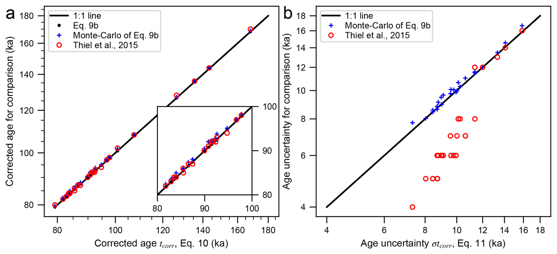
Figure 2 (a) Comparison of our new explicit Eqs. (10) and (11) to former approaches, as demonstrated on the data of Thiel et al. (2015). (a) Age from the explicit Eq. (10) vs. the implicit age from Eq. (9) both as a single-instance (black dots) and averaged Monte-Carlo simulations (blue crosses), and published results (red circles). (b) Age uncertainty from the explicit Eq. (11) vs. standard deviation from Monte-Carlo simulations (blue crosses), and published results (red circles). See Appendix B for tabulated values.

We test our new formulas on the extensive sedimentary archive of Thiel et al. (2015), consisting of 25 feldspar pIR-IR₂₂₅ ages from Oga peninsula (Japan), where D_e, g, and ${\dot{D}}_{\mathrm{nat}}$ and their uncertainties have all been measured and reported (Appendix A). To evaluate W₋₁(x) in Eq. (10), we use SciPy's implementation of Lambert's W function (Virtanen et al., 2020, and references therein). Our Eqs. (9)–(10) yield identical results within 16-digit numerical precision (Fig. 2a), whose relative sub-percent deviation (−0.3 % on average) from Thiel et al. (2015)'s ages is the direct result of the latter's reporting of ages in [ka] units with zero significant digits. The negligible deviation of Monte-Carlo age estimates (−0.67 % on average) from the analytical equations confirms that the effects of measurement uncertainties (σD_e, σg, and $\mathit{\sigma }{\dot{D}}_{\mathrm{nat}}$) propagate linearly into the age correction. Figure 2b demonstrates that Eq. (11) matches Monte-Carlo estimates of age uncertainties across almost an octave of σt_corr within high accuracy (2.6 % on average). Conversely, the age uncertainties reported by Thiel et al. (2015) (red circles Fig. 2b) are not only visibly rounded to the nearest integers, but they progressively underestimate (by up to a factor of 2) the actual age uncertainties with younger age. The latter artefact arises from the community's most popular fading-correction spreadsheet, developed by Sebastian Huot, which is almost never credited (see Jaiswal et al., 2009 for a refreshing exception). In that otherwise excellent spreadsheet, propagation of age uncertainties is done via a finite number of calculated end-member scenarios, which may be insufficient for younger ages vis-à-vis the analytical approach of Eq. (11).

3.2 Lamothe et al. (2003) and Wallinga et al. (2007)

Neither the original “dose response curve” (DRC) correction due to Lamothe et al. (2003), nor its later rendition in Wallinga et al. (2007), amount to new mathematical models per se. Both should instead be thought of as specific applications of the Huntley and Lamothe (2001) correction scheme, each on a different part of the data. The age gain in Lamothe et al. (2003) and Wallinga et al. (2007) relative to Huntley and Lamothe (2001) arises (a) only beyond the linear region of the dose response curve, and (b) solely from the implicit step of nonlinear dose response inversion (Wallinga et al., 2007). This is so because the fading model common to all three papers is agnostic to dose.

Specifically, it can be shown that the age correction of Lamothe et al. (2003) is equivalent to the first iteration of Eq. (9a) with C=0, where the fraction $t_{\mathrm{corr}}/t_{\mathrm{lab}}$ is rewritten as $\frac{D_{\mathrm{e}}/t_{\mathrm{lab}}}{D_{\mathrm{e}}/t_{\mathrm{corr}}}$, in which the numerator and denominator were further described as “laboratory-effective” and “natural” dose rates, respectively (see code Figure_3.py in the Supplement, which calculates the fading corrected age of the sample given in Sect. 4 of Lamothe et al. (2003)). Further support to the claim that Lamothe's DRC-correction is Eq. (9a) in disguise includes the emphasis of Lamothe et al. (2003) on the fact that their expression doesn't require iteration, as well as their Table 1, where the offsets of their DRC correction scheme from that of Huntley and Lamothe (2001) are both negligible ($-\mathrm{0.7}\pm \mathrm{0.8}\mathit{\%}$ on average), and furthermore inconsistent (randomly over- or underestimating Eq. 9a), both of which are hallmarks of a first iteration of a rapidly converging implicit equation (cf. Dodson, 1973).

In a cardinally different approach, only mentioned in passing by Lamothe et al. (2003) but first put into practice by Wallinga et al. (2007), it is the laboratory-regenerated signals which are progressively corrected downwards over time, according to the expected degree of fading that would occur, had the laboratory doses been delivered over a factor ${\dot{D}}_{\mathrm{lab}}/{\dot{D}}_{\mathrm{nat}}$ longer timescale, i.e. if exposed to a natural dose rate. As before, it is the same familiar correction (Eq. 9) which is applied. However, whether or not calculated iteratively, the procedure of Wallinga et al. (2007) brings about a nonlinear deformation the dose response curve itself, resulting in a necessarily older interpolated natural dose, and hence, age, even if one restricts oneself to the linear part of the dose response. The latter distinction is so subtle, that these two distinctly different calculation schemes are nevertheless referred to by the same name (DRC-correction).

To demonstrate the crux of each of these approaches, we use data from Thiel et al. (2015), namely the post-IR225 natural Ln/Tn, dose response, and the reported g-value of K-feldspar sample 055231. The black symbols in Fig. 3a correspond to the raw data; to obtain the uncorrected equivalent dose, the laboratory portion of these data is fitted with a saturating exponential (continuous black line), onto which the natural signal is projected (dashed black line). The Lamothe et al. (2003) correction, as demonstrated in their paper, reiterated in Auclair et al. (2007), and implemented in the R Luminescence package (Kreutzer and Mercier, 2026) affects the natural signal alone, while keeping the dose response curve intact (cf. Fig. 5 in Auclair et al., 2007). Namely, the natural intensity is corrected via a single iteration of Eq. (9a) (blue circle), after which it is projected onto the same dose response as before, yielding a higher equivalent dose (dashed blue line). The approach of Wallinga et al. (2007) is to keep the natural signal as is, but use Eq. (9) to adjust all laboratory-regenerated signals to a timescale longer by factor ${\dot{D}}_{\mathrm{lab}}/{\dot{D}}_{\mathrm{nat}}$, rescaling the luminescence response to that, which the sample would experience if one could “replay” the geological history in real time (red circles). An uncorrected natural signal is then projected onto a different, “faded” dose response curve (red curve). Such a projected equivalent dose is by design larger than that obtained via the verbatim Lamothe et al. (2003) correction, as may be seen on Fig. 3b, where the ratio of the corrected vs. uncorrected dose response curves is plotted, and is seen to be non-linear, progressively decreasing at larger times. In essence, the faded $L_x/T_x$ represents the projected convolution of signal accumulation and loss, rescaled from a laboratory to the natural timescale. Given the algorithmic opacity of Lamothe et al. (2003), these two numerically distinguishable approaches (red and blue lines in Fig. 3a) have been referred to as the “DRC-correction” in the literature, to an extent where the actual calculation scheme is virtually unknowable, despite thorough supplementary data (e.g. Tanski et al., 2025). In this work, we propose to distinguish the Lamothe et al. (2003) correction from the correction scheme of Wallinga et al. (2007), where the natural signal is untouched and it is namely the laboratory dose response which gets stretched and rescaled onto geological timescales, thus paving the way to the more popular Kars et al. (2008) correction as discussed next.

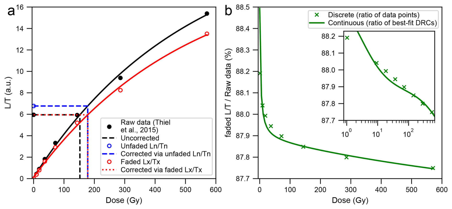
Figure 3 (a) Dose response curve of pIR225 signal of sample 055231 from Thiel et al. (2015), including raw data and uncorrected De (black symbols and curves), as well as corrections using Lamothe et al. (2003) (blue symbols and curves) and Wallinga et al. (2007) (red symbols and curves). (b) The Wallinga et al. (2007) correction affects signals nonlinearly with dose, thereby necessarily interpolating onto larger doses.

3.3 Kars et al. (2008)

Kars et al. (2008) coupled the model of Huntley (2006) to trap repopulation via the environmental dose rate ${\dot{D}}_{\mathrm{nat}}$ under the effect of a saturating exponential growth, where the filling of a finite number of traps N is limited by the characteristic dose D₀, which can be thought of as the e-folding radiation dose absent any fading effects. Recasting Kars' model into a single semi-analytical equation, one obtains:

$$\begin{array}{}\text{(12)}& \begin{array}{rl}{\displaystyle \frac{n\left(t\right)}{N}}& =\underset{\mathrm{0}}{\overset{\mathrm{\infty }}{\int }}{\displaystyle \frac{\mathrm{3}{r}^{\prime \mathrm{2}}\exp \left(-r^{\prime \mathrm{3}}\right)}{\mathrm{1}+\frac{D_{\mathrm{0}}}{\dot{D}}s\exp \left(-{\mathit{\rho }}^{\prime -\mathrm{1}/\mathrm{3}}{r}^{\prime }\right)}}\\ & \left\{\mathrm{1}-e^{-\left[\dot{D}/D_{\mathrm{0}}+s\exp \left(-{\mathit{\rho }}^{\prime -\mathrm{1}/\mathrm{3}}{r}^{\prime }\right)\right]t}\right\}\mathrm{d}{r}^{\prime }.\end{array}\end{array}$$

(cf. Eq. 17 in Li and Li, 2008). To be truly accurate and pedantic, the age correction due to Kars et al. (2008) should be formally written as:

$$\begin{array}{}\text{(13)}& \begin{array}{rl}\underset{\mathrm{0}}{\overset{\mathrm{\infty }}{\int }}& {\displaystyle \frac{\mathrm{3}{r}^{\prime \mathrm{2}}\exp \left(-r^{\prime \mathrm{3}}\right)}{\mathrm{1}+\frac{D_{\mathrm{0}}}{{\dot{D}}_{\mathrm{lab}}}s\exp \left(-{\mathit{\rho }}^{\prime -\mathrm{1}/\mathrm{3}}{r}^{\prime }\right)}}\\ & \left\{\mathrm{1}-e^{-\left[{\dot{D}}_{\mathrm{lab}}/D_{\mathrm{0}}+s\exp \left(-{\mathit{\rho }}^{\prime -\mathrm{1}/\mathrm{3}}{r}^{\prime }\right)\right]D_{\mathrm{e}}/{\dot{D}}_{\mathrm{lab}}}\right\}\mathrm{d}{r}^{\prime }\\ & =\underset{\mathrm{0}}{\overset{\mathrm{\infty }}{\int }}{\displaystyle \frac{\mathrm{3}{r}^{\prime \mathrm{2}}\exp \left(-r^{\prime \mathrm{3}}\right)}{\mathrm{1}+\frac{D_{\mathrm{0}}}{{\dot{D}}_{\mathrm{nat}}}s\exp \left(-{\mathit{\rho }}^{\prime -\mathrm{1}/\mathrm{3}}{r}^{\prime }\right)}}\\ & \left\{\mathrm{1}-e^{-\left[{\dot{D}}_{\mathrm{nat}}/D_{\mathrm{0}}+s\exp \left(-{\mathit{\rho }}^{\prime -\mathrm{1}/\mathrm{3}}{r}^{\prime }\right)\right]t_{\mathrm{corr}}}\right\}\mathrm{d}{r}^{\prime }\end{array}\end{array}$$

where on the left-hand side we have fading-affected signal growth in the laboratory, to be matched by the term on the right-hand side, where fading affected growth to the same level occurs at an environmental dose rate during an unknown duration t_corr. As we show below, Eqs. (12)–(13) lack an exact solution, but are amenable to approximation if we extend the concept of effective radius $r_{\mathrm{eff}}^{\prime }$ as follows. A foreshadowing of our new approximation is to be found in King et al. (2016), whose ansatz multiplied the laboratory dose response curve $\left(\mathrm{1}-e^{-{\dot{D}}_{\mathrm{lab}}t/D_{\mathrm{0}}}\right)$ by Eq. (7) to obtain:

$$\begin{array}{}\text{(14)}& \begin{array}{rl}{\displaystyle \frac{n\left(t\right)}{N}}& =\left[\mathrm{1}-\exp \left(-{\displaystyle \frac{\dot{D}t}{D_{\mathrm{0}}}}\right)\right]\underset{r_{\mathrm{eff}}^{\prime }}{\overset{\mathrm{\infty }}{\int }}\mathrm{3}{r}^{\prime \mathrm{2}}\exp \left(-r^{\prime \mathrm{3}}\right)\mathrm{d}{r}^{\prime }\\ & \cong \left[\mathrm{1}-\exp \left(-{\displaystyle \frac{\dot{D}t}{D_{\mathrm{0}}}}\right)\right]\exp \left[-{\mathit{\rho }}^{\prime }{\ln }^{\mathrm{3}}\left(\mathrm{1.8}s{t}^{*}\right)\right]\end{array}\end{array}$$

where t^* was taken to be half the irradiation time (Aitken 1985, pp. 279–280). Essentially, this is analogous to the Wallinga et al. (2007) approach, only using NND instead of logarithmic decay. The approximation in Eq. (14) is typically satisfactory for t<10⁴ s, but at longer times often results in an unphysical artefact of signal decay (e.g. Supplement Figs. S2B and S3B in King et al., 2016; Fig. 3B and E in Bouscary and King, 2024), arising from the last exponential term in Eq. (14), which at long enough times brings $n\left(t\right)/N$ to zero (no such term exists on the exact, left-hand side of Eq. 14). This artefact can be easily mitigated if we approximate $r_{\mathrm{eff}}^{\prime }\cong {\mathit{\rho }}^{\prime \mathrm{1}/\mathrm{3}}\ln \left(\mathrm{1.8}s\frac{D_{\mathrm{0}}}{\dot{D}}\left[\mathrm{1}-\exp \left(-\frac{\dot{D}t}{D_{\mathrm{0}}}\right)\right]\right)$, from which it follows that at short times, $r_{\mathrm{eff}}^{\prime }(t\to \mathrm{0})\cong {\mathit{\rho }}^{\prime \mathrm{1}/\mathrm{3}}\ln \left(\mathrm{1.8}st\right)$, reducing $r_{\mathrm{eff}}^{\prime }$ to Huntley's formulation (2006), while at long times, $r_{\mathrm{eff}}^{\prime }\left(t\to \mathrm{\infty }\right)\cong {\mathit{\rho }}^{\prime \mathrm{1}/\mathrm{3}}\ln \left(\mathrm{1.8}s{D}_{\mathrm{0}}/\dot{D}\right)$, representing a “frozen” fading front counteracted by trap refilling at a commensurate rate. Substituting our alternative definition of $r_{\mathrm{eff}}^{\prime }$ into Eq. (13) we get:

$$\begin{array}{}\text{(15)}& \begin{array}{rl}{\displaystyle \frac{n\left(t\right)}{N}}& \cong [\mathrm{1}-\exp (-{\displaystyle \frac{\dot{D}t}{D_{\mathrm{0}}}}\left)\right]\exp (-{\mathit{\rho }}^{\prime }{\ln }^{\mathrm{3}}\\ & \mathit{\left\{}\mathrm{1.8}s{\displaystyle \frac{D_{\mathrm{0}}}{\dot{D}}}\right[\mathrm{1}-\exp (-{\displaystyle \frac{\dot{D}t}{D_{\mathrm{0}}}})\left]\mathit{\right\}}).\end{array}\end{array}$$

which for typical parameters matches numerical integration of Eq. (12) to within sub-percent accuracy. By equating two instances of Eq. (15), one for natural $\dot{D}={\dot{D}}_{\mathrm{nat}}$, and the other for laboratory $\dot{D}={\dot{D}}_{\mathrm{lab}}$ growth (cf. Eq. 13), and further approximating $\mathrm{1}-e^{-{\dot{D}}_{\mathrm{nat}}{t}_{\mathrm{corr}}/D_{\mathrm{0}}}\approx \mathrm{1}-e^{-D_e/D_{\mathrm{0}}}$, we obtain:

$$\begin{array}{}\text{(16)}& \begin{array}{rl}{t}_{\mathrm{corr}}& =-{\displaystyle \frac{D_{\mathrm{0}}}{{\dot{D}}_{\mathrm{nat}}}}\ln \mathit{\{}\mathrm{1}-(\mathrm{1}-e^{-\frac{D_{\mathrm{e}}}{D_{\mathrm{0}}}})\\ & {\displaystyle \frac{\exp [-{\mathit{\rho }}^{\prime }{\ln }^{\mathrm{3}}(\mathrm{1.8}s\frac{D_{\mathrm{0}}}{{\dot{D}}_{\mathrm{lab}}}(\mathrm{1}-e^{-\frac{D_{\mathrm{e}}}{D_{\mathrm{0}}}})\left)\right]}{\exp [-{\mathit{\rho }}^{\prime }{\ln }^{\mathrm{3}}(\mathrm{1.8}s\frac{D_{\mathrm{0}}}{{\dot{D}}_{\mathrm{nat}}}(\mathrm{1}-e^{-\frac{D_{\mathrm{e}}}{D_{\mathrm{0}}}})\left)\right]}}\mathit{\}}.\end{array}\end{array}$$

As with Eq. (10), we rewrite Eq. (16) more compactly, which allows us to derive its analytical uncertainty propagation more easily:

$$\begin{array}{}\text{(17)}& \begin{array}{rl}& t_{\mathrm{corr}}=-{\displaystyle \frac{D_{\mathrm{0}}}{{\dot{D}}_{\mathrm{nat}}}}\ln \left(\mathrm{1}-r{n}_e\right),\\ & r=e^{-{\mathit{\rho }}^{\prime }\left[{\ln }^{\mathrm{3}}\left(\mathrm{1.8}s\frac{D_{\mathrm{0}}}{{\dot{D}}_{\mathrm{lab}}}{n}_e\right)-{\ln }^{\mathrm{3}}\left(\mathrm{1.8}s\frac{D_{\mathrm{0}}}{{\dot{D}}_{\mathrm{nat}}}{n}_e\right)\right]},n_e=\left(\mathrm{1}-e^{-\frac{D_{\mathrm{e}}}{D_{\mathrm{0}}}}\right).\\ & {\displaystyle \frac{\mathrm{d}{t}_{\mathrm{corr}}}{d{\mathit{\rho }}^{\prime }}}={\displaystyle \frac{-D_{\mathrm{0}}{n}_{e}r}{{\dot{D}}_{\mathrm{nat}}\left(\mathrm{1}-n_{e}r\right)}}\left[{\ln }^{\mathrm{3}}\left(\mathrm{1.8}s{\displaystyle \frac{D_{\mathrm{0}}}{{\dot{D}}_{\mathrm{lab}}}}{n}_e\right)-{\ln }^{\mathrm{3}}\left(\mathrm{1.8}s{\displaystyle \frac{D_{\mathrm{0}}}{{\dot{D}}_{\mathrm{nat}}}}{n}_e\right)\right].\\ & {\displaystyle \frac{\mathrm{d}{t}_{\mathrm{corr}}}{d{D}_{\mathrm{0}}}}=-{\displaystyle \frac{\ln \left(\mathrm{1}-n_{e}r\right)}{{\dot{D}}_{\mathrm{nat}}}}-{\displaystyle \frac{D_{\mathrm{e}}\left(\mathrm{1}-n_e\right)r}{D_{\mathrm{0}}{\dot{D}}_{\mathrm{nat}}\left(\mathrm{1}-n_{e}r\right)}}\\ & -\mathrm{3}{\mathit{\rho }}^{\prime }r{\displaystyle \frac{n_e-D_e(\mathrm{1}-n_e)/D_{\mathrm{0}}}{{\dot{D}}_{\mathrm{nat}}(\mathrm{1}-n_{e}r)}}\left[{\ln }^{\mathrm{2}}\right(\mathrm{1.8}s\frac{D_{\mathrm{0}}}{{\dot{D}}_{\mathrm{lab}}}{n}_e)-{\ln }^{\mathrm{2}}(\mathrm{1.8}s\frac{D_{\mathrm{0}}}{{\dot{D}}_{\mathrm{nat}}}{n}_e\left)\right].\\ & \mathit{\sigma }{t}_{\mathrm{corr}}=\sqrt{t_{\mathrm{corr}}^{\mathrm{2}}\left[{\left({\displaystyle \frac{\mathit{\sigma }{D}_{\mathrm{e}}}{D_{\mathrm{e}}}}\right)}^{\mathrm{2}}+{\left({\displaystyle \frac{\mathit{\sigma }{\dot{D}}_{\mathrm{nat}}}{{\dot{D}}_{\mathrm{nat}}}}\right)}^{\mathrm{2}}\right]+{\left({\displaystyle \frac{\mathrm{d}{t}_{\mathrm{corr}}}{\mathrm{d}{\mathit{\rho }}^{\prime }}}\cdot \mathit{\sigma }{\mathit{\rho }}^{\prime }\right)}^{\mathrm{2}}}\\ & \stackrel{\mathrm{‾}}{+{\left({\displaystyle \frac{\mathrm{d}{t}_{\mathrm{corr}}}{\mathrm{d}{D}_{\mathrm{0}}}}\cdot \mathit{\sigma }{D}_{\mathrm{0}}\right)}^{\mathrm{2}}}.\end{array}\end{array}$$

Figure 4 (a) Comparison of our new explicit Eqs. (16) and (17) to former approaches, as demonstrated on the data of Thiel et al. (2015). (a) Age from the explicit Eq. (16) vs. the implicit age from Eq. (13) both as a single-instance (black dots) and averaged Monte-Carlo simulations (blue crosses), and published results (red circles). (b) Age uncertainty from the explicit Eq. (17) vs. standard deviation from Monte-Carlo simulations (blue crosses), and published results (red circles). See Appendix B for tabulated values.

We test our new formulas on the same dataset as before, using an “unfaded” estimate of D₀= 476 Gy (cf. Fig. 5b in Sect. 4 below). The relative accuracy of the Kars model approximation (Eq. 16) vis-à-vis the exact numerical quadrature of the Kars et al. (2008) model (Eq. 13) is 0.5 % (Fig. 4a). As in Fig. 2a, Fig. 4 too shows only a negligible deviation of Monte-Carlo age estimates (−0.25 % on average) from the analytical equations. A systematic model-to-model offset, whereby Kars et al. (2008) yields 8.8 ± 1.6 % older ages than the Huntley and Lamothe (2001), is apparent. For discussion on age accuracy vis-à-vis independent constraints (“which model is right?”), we refer the reader to Sect. 4.4. Furthermore, Fig. 4b demonstrates that σt_corr values obtained using Eq. (17) underestimate Monte-Carlo estimates by 4.7 ± 1.5 %, which we still consider as an excellent achievement, given that until now, there existed no alternatives to Monte-Carlo simulations for the estimation of the age uncertainties of the Kars et al. (2008) age correction. We note that even higher accuracy of ${\mathit{\sigma }}_{t_{\mathrm{corr}}}$ in Eq. (17) can be obtained by accounting for $\partial t_{\mathrm{corr}}/\partial D_e$ and $\partial t_{\mathrm{corr}}/\partial {\dot{D}}_{\mathrm{nat}}$ beyond the linear response approximation (the two terms in the square brackets).

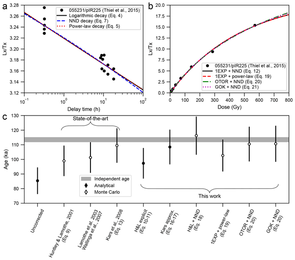
Figure 5 (a) Laboratory decay and (b) Dose response curve of pIR225 signal of sample 055231 from Thiel et al. (2015). (c) Luminescence ages following corrections considered in this study. The horizontal line corresponds to the independent age of 112–115 ka associated with the Toya tephra (Thiel et al., 2015 and references therein).

4 Unorthodox age corrections

By disentangling the fundamental concepts related to quantification of fading rates (Sect. 2) and their derivative age corrections (Sect. 3), we recognize two straightforward model combinations that for some reason have never been put together before (Sect. 4.1 and 4.2 below).

4.1 Age correction from NND decay

The following correction is similar to that of Huntley and Lamothe (2001) in that it uses the quantified fading rate to roll the time back to estimate n₀, yet instead of a formal integration over the burial history assuming logarithmic decay, Eq. (18) is only an ansatz, where the apparent faded age $D_{\mathrm{e}}/{\dot{D}}_{\mathrm{nat}}$ is divided by Eq. (7):

$$\begin{array}{}\text{(18)}& t_{\mathrm{corr}}={\displaystyle \frac{D_{\mathrm{e}}/{\dot{D}}_{\mathrm{nat}}}{\exp \left[-{\mathit{\rho }}^{\prime }{\ln }^{\mathrm{3}}\left(\mathrm{1.8}s{t}_{\mathrm{corr}}\right)\right]}}.\end{array}$$

Equation (18) is analogous to Eq. (9), without rescaling of the g-value (since ρ^′ is a global parameter). Like Eq. (9), Eq. (18) too is implicit with respect to t_corr, but converges quickly via fixed-point iteration (i.e. an iterative procedure, where the left-hand side is updated by substituting its previous value into the right-hand side; initial guess for t_corr is $D_{\mathrm{e}}/{\dot{D}}_{\mathrm{nat}}$).

4.2 Saturating exponential signal growth, coupled to power law decay

The following correction is similar to that of Kars et al. (2008) in that it combines both signal growth and decay, yet instead of using a distribution of traps in combination with the NND model, here charge accumulates in a single trap (first term in parentheses), and decays from it following power law (Eq. 5):

$$\begin{array}{}\text{(19)}& {\displaystyle \frac{n\left(t\right)}{N}}=\left(\mathrm{1}-e^{-\frac{\dot{D}}{D_{\mathrm{0}}}t}\right)\exp \left[-\mathit{\kappa }\ln \left({\displaystyle \frac{t}{t_{\mathrm{c}}}}\right)\right].\end{array}$$

Equation (19) is written as an ansatz (growth × decay). Note the conceptual similarity of Eq. (19) with Eq. (15). To use Eq. (19) to correct an age, one equates between the signal obtained in the laboratory (left hand side below) and in nature (left hand side below), and solves for t_corr:

$$\begin{array}{ll}{\displaystyle }(\mathrm{1}& {\displaystyle }-e^{-\frac{D_{\mathrm{e}}}{D_{\mathrm{0}}}}\left)\exp \right[-\mathit{\kappa }\ln \left({\displaystyle \frac{D_{\mathrm{e}}/{\dot{D}}_{\mathrm{lab}}}{t_{\mathrm{c}}}}\right)]\\ {\displaystyle }& {\displaystyle }=(\mathrm{1}-e^{-\frac{{\dot{D}}_{\mathrm{nat}}}{D_{\mathrm{0}}}{t}_{\mathrm{corr}}})\exp [-\mathit{\kappa }\ln ({\displaystyle \frac{t_{\mathrm{corr}}}{t_{\mathrm{c}}}}\left)\right].\end{array}$$

4.3 Non-first order signal growth, coupled to NND decay

Starting with the model of Kars et al. (2008), we can replace their first-order rate equation to the one-trap one-recombination center (OTOR) model (Pagonis et al., 2020), yielding:

$$\begin{array}{}\text{(20)}& \begin{array}{rl}{\displaystyle \frac{n\left(t\right)}{N}}& =\underset{\mathrm{0}}{\overset{\mathrm{\infty }}{\int }}\mathrm{3}{r}^{\prime \mathrm{2}}\exp \left(-r^{\prime \mathrm{3}}\right){\widehat{n}}_{r^{\prime }}\mathrm{d}{r}^{\prime },\\ {\displaystyle \frac{\mathrm{d}{\widehat{n}}_{r^{\prime }}}{\mathrm{d}t}}& ={\displaystyle \frac{\dot{D}}{D_{\mathrm{0}}}}\cdot {\displaystyle \frac{\mathrm{1}-{\widehat{n}}_{r^{\prime }}}{R+(\mathrm{1}-R){\widehat{n}}_{r^{\prime }}}}-s\exp \left(-{\mathit{\rho }}^{\prime -\mathrm{1}/\mathrm{3}}{r}^{\prime }\right){\widehat{n}}_{r^{\prime }}\end{array}\end{array}$$

where R is a dimensionless retrapping ratio (Pagonis et al., 2020). Note that since a special case of Eq. (20) with R=1 amounts to the Kars et al. (2008) correction (cf. Eq. 12), Eq. (20) can be considered as a direct extension of the Kars et al. (2008) age correction scheme for cases where signal growth complies with the OTOR model. As a counterpart for Eq. (20), and purely for completeness (rather than novelty), we note an earlier and similar attempt at replacing first-order behavior with the general order kinetics (GOK) model (cf. Guralnik et al., 2015a):

$$\begin{array}{}\text{(21)}& \begin{array}{rl}{\displaystyle \frac{n\left(t\right)}{N}}& =\underset{\mathrm{0}}{\overset{\mathrm{\infty }}{\int }}\mathrm{3}{r}^{\prime \mathrm{2}}\exp \left(-r^{\prime \mathrm{3}}\right){\widehat{n}}_{r^{\prime }}\mathrm{d}{r}^{\prime },\\ {\displaystyle \frac{\mathrm{d}{\widehat{n}}_{r^{\prime }}}{\mathrm{d}t}}& ={\displaystyle \frac{\dot{D}}{D_{\mathrm{0}}}}{\left(\mathrm{1}-{\widehat{n}}_{r^{\prime }}\right)}^{\mathit{\alpha }}-s\exp \left(-{\mathit{\rho }}^{\prime -\mathrm{1}/\mathrm{3}}{r}^{\prime }\right){\widehat{n}}_{r^{\prime }}\end{array}\end{array}$$

which conveniently reduces to the Kars et al. (2008) scheme given α=1. Note that while Eq. (21) has been initially introduced within luminescence thermochronology (cf. Sect. 5) it has been shown to perform well also for age correction in sedimentary dating contexts (King et al., 2018). To use Eqs. (20) or (21) to correct an age, one equates two instances of the relevant equation (cf. Sect. 4.2), one expressing laboratory growth and the other growth in nature for an unknown duration t_corr, that one then solves for.

4.4 Benchmarking unorthodox vs. common age corrections vis-à-vis an independent age

The stratigraphic section studied by Thiel et al. (2015) contains two independently dated tephra markers which are widespread in northern Japan, namely the Toya ash (dated by various U-Pb and U-Th methods to ∼ 0.1 Ma with a ∼ 10 % relative uncertainty; see Ito, 2024, and references therein) and the Aso-4 tephra (whose radiometric K-Ar age is 89±7 ka; Matsumoto, 1990). The only sample in Thiel et al. (2015) with sufficiently documented raw luminescence data to enable full age recalculation using all the approaches presented in this paper, is sample 055231, directly capped by the Toya ash. The raw fading data of sample 055231/pIR225 (circles in Fig. 5a) are fitted using models discussed in Sect. 2 (lines in Fig. 5a). Here it is timely to note that unlike in Fig. 5b, the scatter of fading data around either of the models in Fig. 5a raises serious methodological doubt regarding the quality of the fitted dataset itself; regretfully, transparent discussion on the design of fading measurement experiments has been uncommon since Auclair et al. (2003). The raw dose response data of sample 055231/pIR225 (circles in Fig. 5b) are fitted using models discussed in Sects. 3–4 (curves in Fig. 5b), i.e. incorporating the overprinting of the quantified fading from Fig. 5a onto the dose response behavior. Unlike in Fig. 5a, there is little scatter of data from its best-fitted model, but the models themselves are equally indistinguishable vis-à-vis the data, just as they were in Fig. 5a. This is also the reason that the two higher-order kinetics models (Eqs. 20–21) are deemed overparametrized with respect to the available data. In other words, the kinetic parameters cannot be extracted from fitting of Eqs. (20)–(21) to the existing data, due to strong parameter covariance. Nevertheless, in order to demonstrate the results of such models if their kinetics could be confidently determined elsewhere, we proceeded with an appreciable retrapping in both (R=0.5 in Eq. 20, and α=2 in Eq. 21), just for illustration purposes.

Figure 5c summarizes the uncorrected age of sample 055231/pIR225 (leftmost symbol) alongside 3 state-of-the-art age corrections (methods already described in the literature), followed by 6 novel approaches presented and discussed in this work. The horizontal line in Fig. 5c is a Toya tephra age of 112–115 ka as assigned by Thiel et al. (2015), from the references that were available to these authors at the time of writing. While model fits to the anomalous decay data (circles in Fig. 5a) and dose response (circles in Fig. 5b) are barely distinguishable, there is a considerable variance in the resulting pIR225 ages (circles with error bars in Fig. 5c), spanning 75–130 ka within 1σ uncertainties.

Within the methodological uncertainties of luminescence dating, the independent 112–115 ka age is matched by any of the physical corrections of IRSL fading (i.e. all except Huntley and Lamothe, 2001, and Lamothe et al., 2003). Note, that the fading corrected ages cluster into two groups, corresponding to the younger ages from non-NND models (Eqs. 9–11 and 19), in contrast to the older ages from the NND decay models (Eqs. 18, 20 and 21); the latter appear to yield results closer to the independent age constraint that Thiel et al. (2015) quoted. It is cautiously remarked that replacing the first-order signal growth of Kars et al. (2008) with either GOK or OTOR (Eqs. 20–21) does not seem to affect model accuracy vis-à-vis the 112–115 ka age reference.

Regrettably, the exercise in Fig. 5c is too limited to draw any substantial conclusions regarding the validity of the anomalous fading corrections being tested, or lack thereof. Even for the reanalyzed sample (055231), Thiel et al. (2015)'s 112–115 ka age bracket is unrealistically narrow in light of the latest and most rigorous geochronological investigation of the Toya ash (Ito, 2024), which cautiously refers to that volcanic event as a ∼ 0.1 Ma eruption with a 1σ age uncertainty of ∼ 10 % (cf. a U-Th isochron age of 110 ± 14 ka, and weighted mean U-Pb age of 103 ± 14 ka). With this latter and more realistic age constraint, any of the fading-corrected luminescence ages in Fig. 5c are in accordance with the best available independent chronology (Ito, 2024).

While we lack dose response data for samples 055255 and 055256 to be able to conduct a similar exercise to that presented in Fig. 5, their results are also of interest and are discussed below. These samples, which bracket the 89 ± 7 ka Aso-4 tephra from just below and above, yield weighted luminescence mean ages of 91.5 ± 10.6 ka using the Huntley and Lamothe (2001) correction, and 99.7 ± 11.6 ka using the Kars et al. (2008) model (Appendix B). Just as with the Toya ash, the independent age constraint doesn't allow discerning “which fading model is right”: within methodological uncertainties, they all are. To explicitly warn the reader against confirmation bias that the Huntley and Lamothe (2001) correction (91.5 ± 10.6 ka) falls “closer” to the K-Ar age, a few caveats regarding age accuracy are given. A potential for a < 5 % systematic age underestimation of the K-Ar system relative to its more accurate ⁴⁰Ar-³⁹Ar successor (Renne, 2006), could easily raise the independent age of the Aso-4 ash to 93.5 ± 7 ka. An analogous but significantly larger systematic overestimation of < 20 %, affecting the luminescence chronometry, is potentially due to severe uncertainties with respect to dose rate $\dot{D}$ (cf. last two columns in Table 1 of Thiel et al., 2015, with Fig. S5 and Table S5 in Guralnik et al., 2015b). In fact, Thiel et al. (2015) explicitly concluded their paper emphasizing “the importance of investigating the mineral composition in more detail in order to get better dose rate estimates”, and it is beyond all doubt that their mineralogical study (their Sect. 3.2 and Fig. 4) arose from an incipient mismatch of their feldspar IRSL ages with independent age control, when standard dose rate calculations led to severe (∼ 20 %) age underestimation vis-à-vis tephrochronology. Increasing all dose rates in Appendix A by even 10 %, the fading-corrected pIR225 ages based on the Huntley and Lamothe (2001) and Kars et al. (2008) corrections would be ∼ 82 and ∼ 89 ka, respectively, with an opposite implication to that from before, i.e. that it is namely the Kars et al. (2008) model, which yields results which are “closer” to the independent K-Ar age.

The analysis above, and the naiveté of some of the strawman arguments presented (which model is “closer” to independent age control), demonstrates that the distinction between different luminescence fading models, even in a “perfect” sedimentary archive with an abundance of solid external chronological constraints, can very quickly run into circular arguments at best. Extreme caution is therefore needed when reconciling between different chronologies (e.g. Guralnik et al., 2011), let alone promoting or dismissing models of one method against results from another – which we simply dare not partake in. In light of the above, we find it necessary to end Sect. 4.4 with a disclaimer, that the aim of the present work has been solely to state all the luminescence fading models in a mathematically literate manner, and present correct and transparent calculations; it is entirely the practitioner's task to use these models responsibly, or as George Box once wittingly remarked, “all models are wrong, but some are useful”.

5 Equilibrium ages

Robust independent age controls for sedimentary deposits are often difficult to establish, because of limited materials available for alternative dating methods, as well as the limitations of those methods themselves (e.g. ∼ 50 ka detection limit of ¹⁴C, potential open-system behavior of U $/$ Th, etc.). In contrast, a thermochronological constraint may offer a simpler case study, for rocks that have experienced isothermal storage of the luminescence system at a temperature, T_nat, for a period greatly exceeding the response time of that system. Due to its tectonic quiescence during the Quaternary, the KTB borehole offers an ideal setting for validation of trapped charged thermochronometers (Guralnik et al., 2015b, and references therein). Eq. (22) below is a crude approximation of combining athermal and thermal losses of a luminescence system to predict its age (cf. Guralnik and Sohbati, 2019):

$$\begin{array}{}\text{(22)}& \begin{array}{rl}& t_{\mathrm{model}}=-{\displaystyle \frac{D_{\mathrm{0}}}{{\dot{D}}_{\mathrm{nat}}}}\ln \left(\mathrm{1}-f_x\mathit{\theta }\right),\\ & \mathit{\theta }={\displaystyle \frac{[\mathrm{1}+{\displaystyle \frac{s_{\mathrm{th}}\exp (-E_{\mathrm{eff}}/k_B{T}_{\mathrm{nat}})}{{\dot{D}}_{\mathrm{nat}}/D_{\mathrm{0}}}}{]}^{-\mathrm{1}}}{[\mathrm{1}+{\displaystyle \frac{s_{\mathrm{th}}\exp (-E_{\mathrm{eff}}/k_B{T}_{\mathrm{lab}})}{{\dot{D}}_{\mathrm{lab}}/D_{\mathrm{0}}}}{]}^{-\mathrm{1}}}}.\end{array}\end{array}$$

where t_model is the model age, f_x is the athermal equilibrium factor, extracted from either Eqs. (10) or (16):

$$\begin{array}{}\text{(23)}& {\displaystyle }\begin{array}{rl}{f}_{\mathrm{H}\mathrm{\&}\mathrm{L}}& ={\displaystyle \frac{\mathrm{2}{\dot{D}}_{\mathrm{lab}}}{{\dot{D}}_{\mathrm{nat}}}}{e}^{-P-Q},P=\mathrm{1}+{\displaystyle \frac{\mathrm{1}}{\mathit{\kappa }}}-\ln {\displaystyle \frac{D_e}{\mathrm{2}{\dot{D}}_{\mathrm{lab}}{t}_c}},\\ Q& =W_{-\mathrm{1}}\left[-{\displaystyle \frac{\mathrm{2}{\dot{D}}_{\mathrm{lab}}}{{\dot{D}}_{\mathrm{nat}}}}(P-\mathrm{1})e^{-P}\right].\end{array}\text{(24)}& {\displaystyle }{f}_{\mathrm{Kars}}={\displaystyle \frac{\exp \left[-{\mathit{\rho }}^{\prime }{\ln }^{\mathrm{3}}\left(zs{D}_{\mathrm{0}}/{\dot{D}}_{\mathrm{nat}}\right)\right]}{\exp \left[-{\mathit{\rho }}^{\prime }{\ln }^{\mathrm{3}}\left(zs{D}_{\mathrm{0}}/{\dot{D}}_{\mathrm{lab}}\right)\right]}}\end{array}$$

while θ is a conceptually identical expression to f_x, yet accounting for thermal equilibrium (cf. Guralnik and Sohbati, 2019).

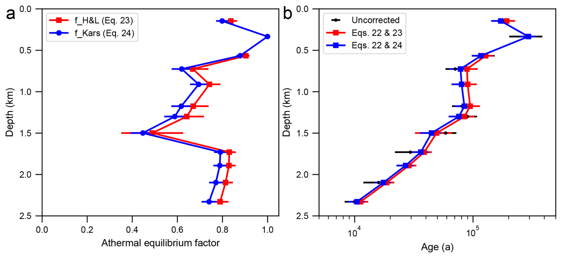
Figure 6 Equilibrium system at the KTB borehole, Germany. (a) Athermal equilibrium factors from Eqs. (23)–(24), alongside thermal equilibrium (continuous curve), as a function of sample depth. (b) observed vs. modelled ages vs. depth.

Figure 6 demonstrates that Eq. (22) can be successfully used to quantitatively predict the observed ages of samples from the KTB borehole (Guralnik et al., 2015b) across a broad range of $g_{\mathrm{2}d}=\mathrm{0}-\mathrm{7}$ % per decade, and ∼ 1.5 orders of magnitudes of apparent age (Appendix C). Note, that in Fig. 6b, the underground and laboratory temperatures obey $T_{\mathrm{nat}}\left(z\right)=\mathrm{7.5}+\mathrm{27.5}z$ [°C] and T_lab=15 °C, respectively, while the thermal stability of the IRSL₅₀ system is approximated as (a) uniform throughout the borehole (cf. Bouscary and King, 2024), and (b) as a first-order system with activation energy of E_eff=0.92 eV and thermal escape frequency s_th=55 s⁻¹ (cf. Guralnik and Sohbati, 2019). Such thermal stability parameters are obviously a generous approximation, given that significant differences in sample-specific E and s_th have been documented (Guralnik et al., 2015b), and given that the mentioned E_eff and s_th are only “apparent” values, averaging over several kinetic processes to and from the excited state of the IRSL electron trap (cf. Guralnik and Sohbati, 2019). Nevertheless, the novelty of Eq. (22) is that it is the first explicit and to-date the most compact model, that can quantitatively predict the observed IRSL₅₀ data at 12 different depths of the KTB site (Appendix D) with a minimum of parameters and input data (Appendix C). The latter is achieved via convolution of two equilibrium factors, one thermal (θ) and one athermal (f), which appears powerful in replacing extensive Monte-Carlo simulations (Guralnik et al., 2015b) with a single and straightforward one-line expression (Eq. 22).

6 Discussion and conclusions

The primary aim of the present contribution is the disentanglement of the mathematical treatment of anomalous fading, where historical inaccuracies have resulted in obfuscated calculation approaches, that even seasoned practitioners have a hard time navigating. Our paper demonstrates that the two most popular fading corrections (Huntley and Lamothe, 2001; Kars et al., 2008) are amenable to a closed-form explicit solutions, which reduce practitioner dependence on computational brute force, and provide mathematical clarity and intuition regarding sensitivity of the fading correction to the various model parameters involved. The validity of our mathematics has been demonstrated via comparison of our new equations vis-à-vis legacy Monte-Carlo approaches in two classic archives, one from a sedimentary sequence (Sect. 4) and another from a thermochronological context (Sect. 5).

While this paper is not aimed at answering the commonly posed question regarding “which model is right”, our present exercise does allow us to make cautious remarks about model validity and applicability. Here, it appears that ages corrected using the Huntley and Lamothe (2001) scheme are systematically younger than those obtained by the Kars et al. (2008) correction, and although this is not a new observation (Kars and Wallinga, 2009), our analysis highlights that this offset has little to do with linearity of signal growth, but rather stems from (a) the unphysical nature of logarithmic loss (Eq. 4), and (b) reflects an arbitrary offset arising from the “−1” term in Eq. (9). These effects (a and b) diminish as soon as the Huntley and Lamothe (2001) core scheme is upgraded to a power-law decay (Eq. 18), which is an overlooked yet necessary outcome of Visocekas (1976, 1985) own quantification of anomalous fading.

Unlike the empirical/heuristic expressions for logarithmic (Eq. 4) or “power law” (Eq. 5) decays, nearest-neighbor distribution decay (Eq. 7) is a physically-driven model, traceable to the now seemingly forgotten research on electron traps in ZnS phosphors (Hoogenstraaten, 1958). In the limited example considered in Sect. 4, we demonstrated that all age corrections utilizing NND decay yielded age estimates consistent with the “conventional” independent age of the sedimentary unit in question. It is important to note, that NND-based models resulted in a cluster of corrected ages, regardless of whether charge retrapping is only implicit (Eq. 18), or whether NND decay was coupled to first-order (Eqs. 13/16–17) or higher-order (Eqs. 20–21) charge retrapping models. The main takeaway from this exercise is that the choice of the particular retrapping model, as methodologically important as it might be, seems to exert only a second-order effect on the fading correction, while NND is the only truly physics-based “anomalous fading” model whose results are in line with independent age control.

From Fig. 4a–b, it is evident that standard laboratory experiments (including the dose response and the isothermal decay of the total target IRSL signal) appear insufficient for confirming or disproving the validity of the various decay and accumulation models discussed – as all the latter fit the available laboratory data equally well. The good news is that luminescence age correction seems to be overall resilient to varying formulations of the trapping-detrapping system (cf. King et al., 2018). The more challenging news is that in order to further increase the accuracy of fading-corrected IRSL ages via a better informed model choice, one will have to either conduct studies in archives where impeccable datasets of independent ages are available (cf. Sect. 4.4 for a cautionary tale), or that a more rigorous laboratory characterization of IRSL signal sub-components will become necessary to both justify and elucidate the parameters of the nonlinear signal growth models (e.g. Eqs. 20–21).

As a final remark, it appears that Eq. (18) is a plausible replacement for the legacy Huntley and Lamothe (2001) age correction, whenever no information on dose response is available, while variants of the Kars et al. (2008) model (Eqs. 13, 16–17, 20–21) can be utilized whenever the luminescence system is suspected to deviate from linear accumulation, en route to signal saturation (or more broadly, field steady-state).

Appendix A

Table A1 Data for samples from Oga peninsula (MIS 5 Japanese marine deposits).

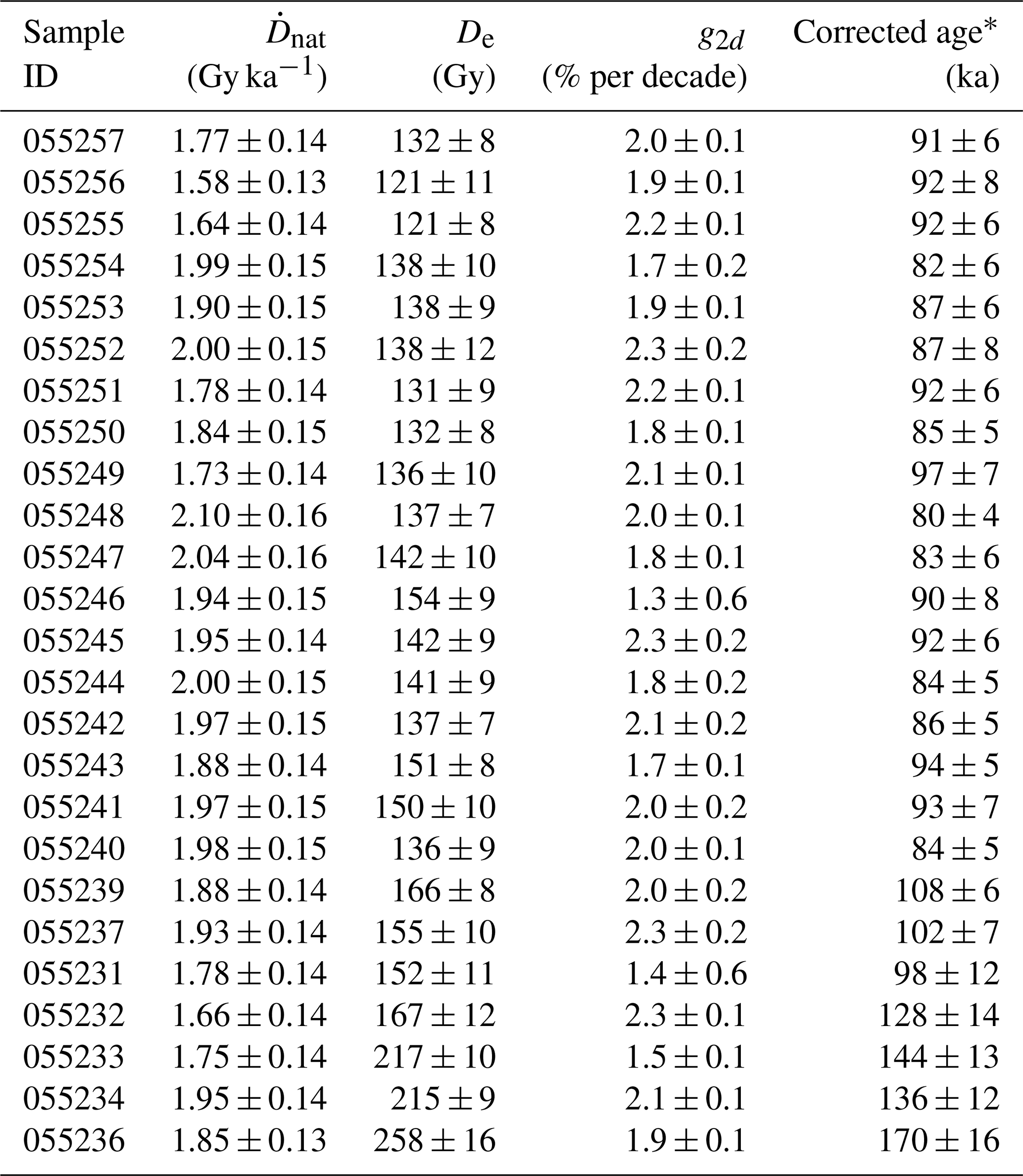
Feldspar post-IR IR₂₂₅ measurements for the sedimentary samples from Thiel et al. (2015). ^* As published (reported using the Huntley and Lamothe (2001) correction).

Appendix B

Table B1 Simulated ages and uncertainties for Oga peninsula (all in units of ka).

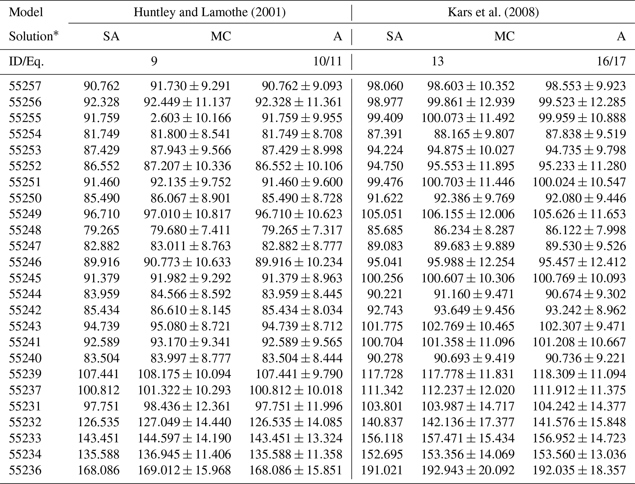
^* SA: semianalytical; MC: Monte-Carlo simulation (N=1000); A: Analytical.

Appendix C

Table C1 Data for samples from the KTB borehole.

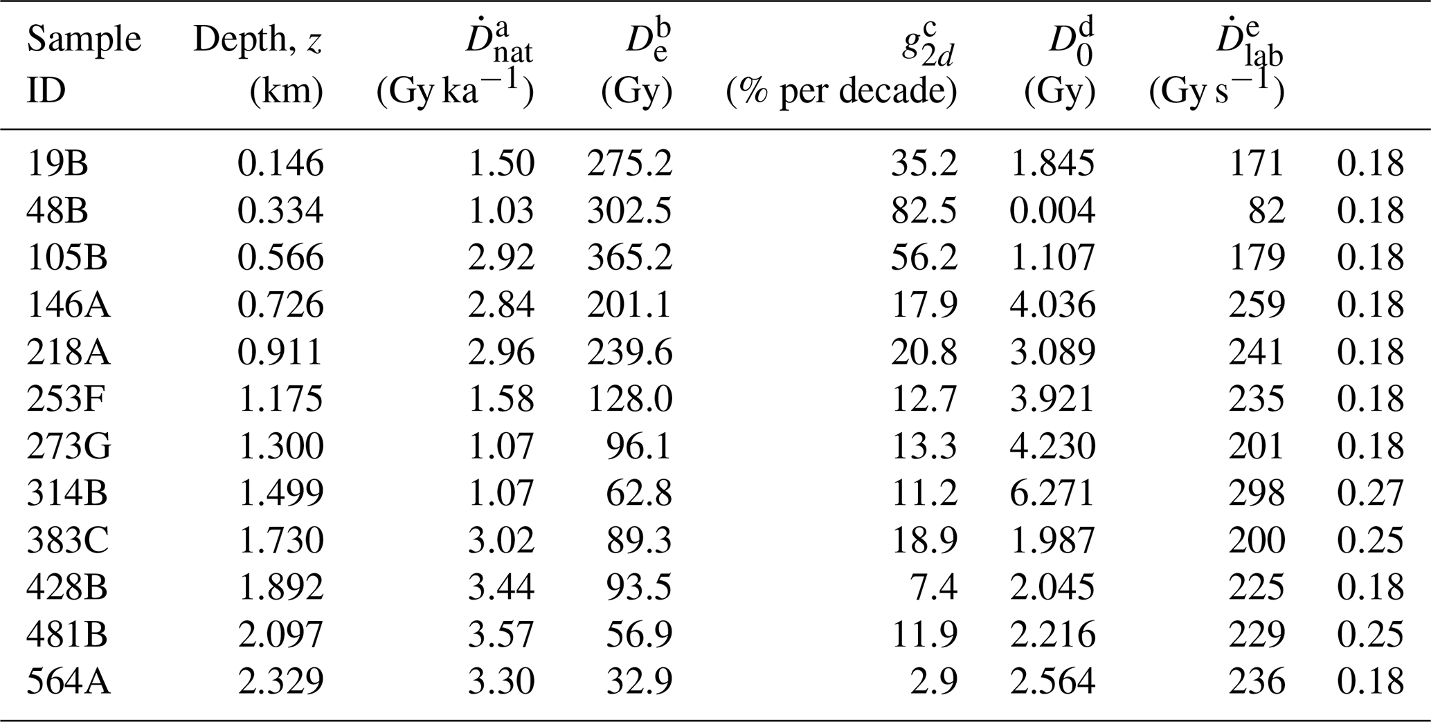
Subsurface bedrock samples from Guralnik et al. (2015b). ^a Assigned 15 % relative uncertainty. ^b Recalculated from the original publication via $D_{\mathrm{e}}=-D_{\mathrm{0}}\ln \left(\mathrm{1}-L_{\mathrm{nat}}/L_{\mathrm{labmax}}\right)$. ^c recalculated using Eq. (5a) from sample-dependent ρ^′ and s values, and assigned 15 % relative uncertainty. ^d assigned 3 % relative uncertainty. ^e the maximum laboratory dose rate (no uncertainties considered).

Appendix D

Table D1 Simulated values for the KTB borehole.

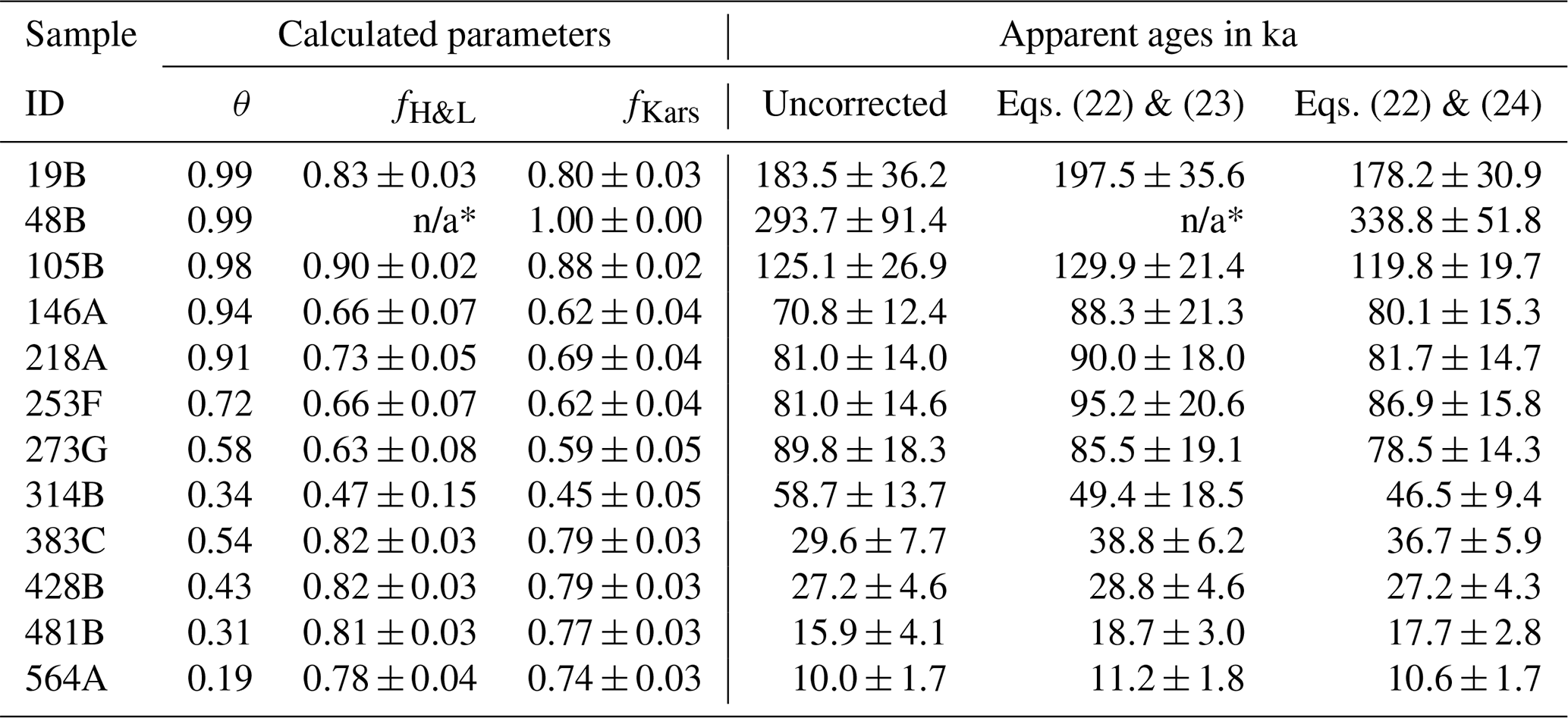
^∗ n/a: not applicable – results in numerical overflow of the Lambert W expression, signifying that the Huntley and Lamothe (2001) correction is degenerate due to a negligible fading rate.