the Creative Commons Attribution 4.0 License.
the Creative Commons Attribution 4.0 License.
 | 21 May 2021
Spatially resolved infrared radiofluorescence: single-grain K-feldspar dating using CCD imaging
Dirk Mittelstraß
Sebastian Kreutzer
The success of luminescence dating as a chronological tool in Quaternary
science builds upon innovative methodological approaches, providing new
insights into past landscapes. Infrared radiofluorescence (IR-RF) on
K-feldspar is such an innovative method that was already introduced two decades
ago. IR-RF promises considerable extended temporal range and a simple
measurement protocol, with more dating applications being published recently.
To date, all applications have used multi-grain measurements. Herein, we take
the next step by enabling IR-RF measurements on a single grain level.
Our contribution introduces spatially resolved infrared
radiofluorescence (SR IR-RF) on K-feldspars and intends to make SR IR-RF
broadly accessible as a geochronological tool. In the first part of the
article, we detail equipment, CCD camera settings and software needed
to perform and analyse SR IR-RF measurements. We use a newly developed
ImageJ macro to process the image data, identify IR-RF emitting
grains and obtain single-grain IR-RF signal curves. For subsequent
analysis, we apply the statistical programming environment R and
the package Luminescence. In the second part of the article, we
test SR IR-RF on two K-feldspar samples. One sample was irradiated
artificially; the other sample received a natural dose. The artificially
irradiated sample renders results indistinguishable from conventional
IR-RF measurements with the photomultiplier tube. The natural sample
seems to overestimate the expected dose by ca. 50 % on average. However,
it also shows a lower dose component, resulting in ages consistent with
the same sample's quartz fraction. Our experiments also revealed an
unstable signal background due to our cameras' degenerated cooling
system. Besides this technical issue specific to the system we used, SR
IR-RF is ready for application. Our contribution provides guidance and
software tools for methodological and applied luminescence (dating)
studies on single-grain feldspars using radiofluorescence.
- Article
(5106 KB) - Full-text XML
-
Supplement
(947 KB) - BibTeX
- EndNote


During the last two decades of advances in luminescence-based chronologies, two promising developments stand out but somehow never took off: (1) spatially resolved (SR) detection of optical and thermoluminescence signals and (2) infrared radiofluorescence (IR-RF) of potassium feldspar (K-feldspar). Our perception is that the most significant obstacles in both approaches lie in imperfections of the available instrumentation and the complexity of the data analysis.
Although aware of this, we draw upon both developments, SR and IR-RF, and present a new approach: spatially resolved infrared radiofluorescence (henceforth: SR IR-RF) for measuring K-feldspar on a single grain level. This article has two parts. After a brief literature review, the first part will outline the technical aspects and the data analysis methods. The second part will test and apply the developed approach.
As it concerns our article's technical part, we attempt to summarise our work on SR IR-RF of K-feldspar carried out since 2015. We will present a detailed workflow, a new software toolchain, guidelines and technical suggestions like the parameterisation of the used EM-CCD camera.
In the application part of our article, we will present a first test of the hypothesis of whether SR IR-RF allows deciphering single feldspar grains' bleaching history. We used a sample from the Médoc area (south-western France) previously dated using non-spatially resolved IR-RF for this test.
1.1 Spatially resolved luminescence dating
Conventional luminescence readers rely on photomultiplier tubes (PMTs) to detect luminescence emissions (e.g. Bortolot, 2000; Bøtter-Jensen et al., 2000; Richter et al., 2015; Maraba and Bulur, 2017). However, equivalent dose (De) distributions deduced from multiple-grain aliquots tend to scatter more than individual analytical uncertainties can explain (for a brief overview on various reasons, see Fitzsimmons, 2019), and a PMT does not allow distinguishing simultaneously emitted signals from individual grains.
Single-grain systems, such as employed by Bøtter-Jensen et al. (2003), use a laser to optically stimulate luminescence (OSL, Huntley et al., 1985) single grains sequentially. Hence, luminescence is collected grain-wise. However, such a system does not suite when (1) the stimulation (heating, irradiation) can only be applied simultaneously to all grains, or (2) spatial mapping of the sample is desired (e.g. Duller and Roberts, 2018). For these reasons, luminescence imaging systems have been subject of research since, at least, the 1980s (cf. Huntley and Kirkley, 1985). In the 1990s, charged coupled device (CCD) cameras became affordable and gained attraction for luminescence detection due to their high quantum efficiency in conjunction with a relatively simple technical implementation into existing systems. A variety of experimental and commercial image systems based on CCD cameras were developed (Duller et al., 1997; Spooner, 2000; Greilich et al., 2002; Baril, 2004; Clark-Balzan and Schwenninger, 2012; Chauhan et al., 2014; Greilich et al., 2015; Kook et al., 2015; Duller et al., 2020). However, the number of publications making use of those systems in the context of actual dating appears to be surprisingly small (e.g. Greilich et al., 2005; Rhodius et al., 2015; Duller et al., 2015).
Reasons for this lag of attention might be found in the technical complexity of luminescence imaging systems, combined with significant issues such as image noise or signal cross-talk (Gribenski et al., 2015; Cunningham and Clark-Balzan, 2017). Thus, luminescence imaging methods appear challenging to apply, and the efforts necessary to analyse the measurements might be considered disproportional to the scientific gain. To prevent spatially resolved IR-RF from failing for the same reasons, we intend to provide our software and methods as accessible, transparent and automated as possible.
1.2 The brief history of spatially resolved IR-RF dating
IR-RF dating applies ionising radiation to stimulate a fluorescence signal in K-feldspar at a wavelength of around 865 nm (Trautmann et al., 1999). This IR-RF signal decays with the accumulation of dose and resets through optical bleaching (e.g. a few hours to days of sunlight exposure). Determining ages up to ca. 600 ka is reported in the literature (Wagner et al., 2010).
The early development of conventional non-spatially resolved IR-RF as dating technique was an effort of the group led by Matthias Krbetschek at the TU Freiberg (Germany) (Trautmann et al., 1998, 1999; Krbetschek et al., 2000; Erfurt and Krbetschek, 2003b). Their work cumulated in the infrared radiofluorescence single aliquot regenerative-dose (IRSAR) protocol (Erfurt and Krbetschek, 2003a). Although the IRSAR protocol is straightforward and promises extended temporal range, its invention had limited impact on the dating practice in Quaternary science (see Murari et al., 2021, for a detailed review).
One particular issue is the low bleachability of the IR-RF signal (at least 2 h of natural sunlight, Trautmann et al., 1999), which potentially provokes partial bleaching effects. Other issues are potential inhomogeneities in the mineral composition and micro-dosimetry of the sample (Trautmann et al., 2000).
Seeking a technical solution, Krbetschek and Degering (2005)1 conducted first spatially resolved (SR) IR-RF measurements on feldspars. In their experiment, the sample was irradiated from below with a 90Sr Y β source. The RF signal was collected by a 45∘ mirror and a custom-made imaging optic, with the signal detected through an electron multiplying (EM) CCD camera. Images were analysed using the software AgesGalore (Greilich et al., 2006).
When Matthias Krbetschek joined Freiberg Instruments GmbH, the capability of performing SR IR-RF measurements became part of the design of the commercial available lexsyg research reader (Richter et al., 2013). Contrary to the original design by Krbetschek and Degering (2005), in this system, the 90Sr Y source is placed above the sample position. A circular opening in the middle of the source module enables luminescence detection (Richter et al., 2012). A sketch of this lexsyg research RF imaging module is shown in Fig. 1. With the early death of M. Krbetschek in 2012, the progression in the SR IR-RF technique's development came to a temporary halt.

Figure 1(a) Technical sketch of the camera system for spatially resolved IR-RF measurements at the lexsyg research reader L2 in Bordeaux. The collimating lens position and the camera's height were adjusted manually to obtain the best IR-RF image quality. (b) Typical image output of a natural IR-RF image stack. The upper picture shows an unprocessed but background-corrected SR IR-RF image taken with high SNR setting (see Table 2). Two speckle noise events caused by bremsstrahlung (white) and two grain IR-RF signals (yellow) are marked. Individual grain signals are hardly distinguishable from the image noise. The lower image shows the processed image stack's median image, where light from individual grains is visible. The dashed white line marks the rim of the sample carrier (here a stainless-steel cup).
In the following section, we outline technical aspects of relevance for successful SR IR-RF measurements. Although we were bounded to tailor some settings to a particular system, the overall parameterisation and the developed workflow is fairly system independent. More detailed information is available in the Appendix and the referenced resources.
2.1 Equipment
All measurements presented in this article were performed on a single Freiberg Instruments lexsyg research reader (Richter et al., 2013) at the IRAMAT-CRP2A in Bordeaux (reader name L2). The system is equipped with a ring-shape type 90Sr Y β source (Richter et al., 2012) delivering ca. 3.5 Gy min−1 to K-feldspar grains with a size of 125–250 µm (cf. Frouin et al., 2017).
For luminescence detection, we used a Princeton Instruments ProEM: 512B+ eXcelon EMCCD camera with a 512×512 pixel unichromatic back-illuminated CCD sensor. The camera sits on an automated detector changer, which allows also for spatially resolved thermal luminescence (TL) and OSL measurements (cf. Richter et al., 2013; Greilich et al., 2015). The camera has a quantum efficiency (QE) of ⩾80 % between 450 and 750 nm. At the K-feldspar IR-RF emission centred at ca. 865 nm the QE is around 60 %. For the IR-RF measurements, we placed a Chroma D850/40x interference filter between β source and EMCCD camera. The custom-made optic has a numerical aperture (NA) of about 0.2 and a lateral magnification of 0.6, leading to an image resolution of 27 µm per pixel. Prior to our experiments, we adjusted the optical focus by manually calibrating the camera's installation height until we obtained the best image quality in terms of sharpness and minimised distortion. The nearby 90Sr Y β source shielding emits secondary X-ray photons (bremsstrahlung, cf. Liritzis and Galloway, 1990), which induce localised high signal events at the CCD chip upon impact. The result is images speckled with bright spots (see Fig. 1b). We will refer to this effect as “speckle noise”. It has to be noted that naturally occurring cosmic rays also cause similar bright spots. However, we approximated that cosmic rays are responsible for less than 1 % of the spots.
The system was equipped with a solar light simulator (SLS) system facilitating LEDs with broad peaks centred at 365, 462, 523, 590, 625 and 850 nm (Richter et al., 2013). The system is the same as used for the experiments by Frouin et al. (2015) and Frouin et al. (2017).
However, over the years, the system received a couple of hardware upgrades tackling various problems (cf. Kreutzer et al., 2017). In 2018, an improved drive train for the sample arm, modernised control hardware and a new 100 W at 48 V Si3N4 heater controlled by a PT1000 thermocouple were installed (personal communication, Freiberg Instruments GmbH, 2019).
2.2 Software
Our software toolchain consisted of three different tools:
LexStudio 2 for measurement sequence control, ImageJ for
image processing and the R function library Luminescence for data
analysis. ImageJ and the Luminescence package are
open-source (GPL-3 licence) and freely available for all major platforms
(Windows, Linux, macOS). However, our software
toolchain was tested so far just on Windows 10 and macOS
(v10–v11). Detailed installation guides and additional download links
to the SR IR-RF-specific software modules can be found at
https://luminescence.de/ (last access: 28 March 2021).
2.2.1 Image acquisition with LexStudio 2
We used the software LexStudio 2 (version 2.5.0, 2019-11-01) shipped with the measurement system for sequence writing, camera parameterisation and image acquisition. For the presented work, Freiberg Instruments updated LexStudio 2 in 2018/2019 with a new module to control the camera settings relevant for luminescence imaging (Fig. 2a). The new module also enables sequence-synchronous camera control and data handling. Thus, sequence writing does not differ from routine luminescence measurements with a PMT. The new LexStudio 2 camera module uses the 32-bit PVCAM drivers by Princeton Instruments and maintains the compatibility to the camera control software WinView shipped with the ProEM camera. Unfortunately, this enhanced version of LexStudio 2 is currently bound to 32-bit Microsoft Windows platforms. The obtained data, however, can be separately processed and analysed on other computers with other platforms. The data consist of one image stack for each RF measurement, saved as a 16-bit greyscale TIF file. To prevent system crashes due to the 3 GB barrier of 32-bit platforms, LexStudio 2 provides an option to split large data sets automatically.
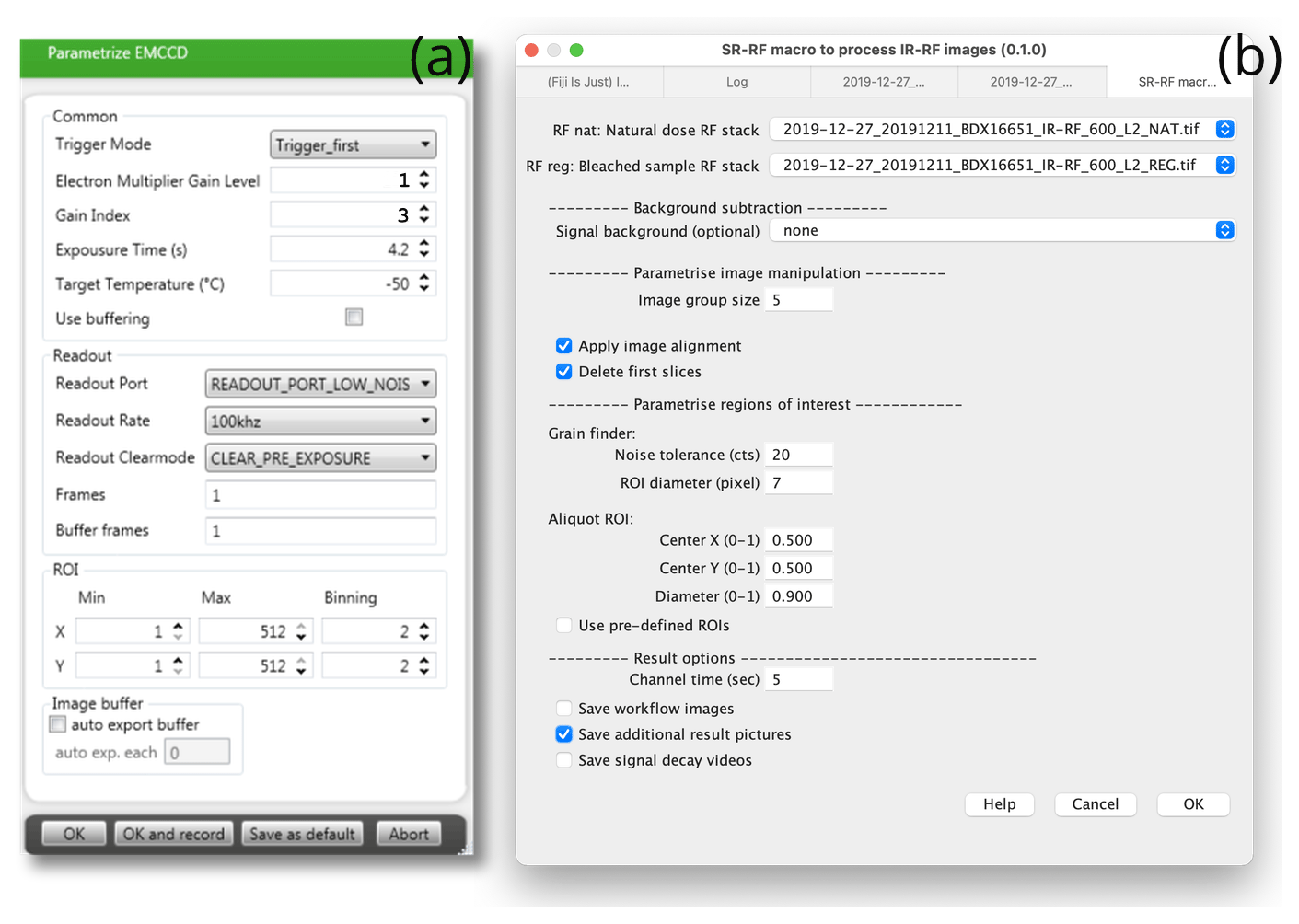
Figure 2Screenshots of (a) the LexStudio 2 interface to parameterise the CCD camera and (b) the SR-RF ImageJ macro interface to analyse IR-RF images.
2.2.2 Image processing with ImageJ
For processing the image data, we used the open-source software
ImageJ (version: 1.52p) (Schneider et al., 2012). We developed
a macro called SR-RF (file SR-RF.ijm, see the Supplement) to
automatise the workflow. The SR-RF macro is a plain ASCII file and
written in the JavaScript-like ImageJ macro language. It provides
a graphical user interface (Fig. 2b) to simplify
user interactions. The output is an ASCII text file with the file-ending
*.rf. The file contains the single-grain IR-RF curves, the size
and spatial location of the associated regions of interests (ROIs) and
further image-processing information. We used the enhanced ImageJ
distribution Fiji (https://fiji.sc, last access: 28 March 2021) (version: 2.0.0-rc-69)
for most of our analyses. A cross-platform version of ImageJ and
the SR-RF macro and all necessary plug-ins pre-installed can be
downloaded from
https://luminescence.de/ (last access: 28 March 2021). A short
description of how to install the SR-RF macro and its dependencies and
detailed documentation of the macro can also be found on our website.
Interfacing of the macro to other programs is possible through the
additionally supported ImageJ batch mode.
2.2.3 Data analysis with R
We employed the statistical programming environment R
(R Core Team, 2020) and the package Luminescence
(Kreutzer et al., 2012, 2020) for processing the IR-RF
single-grain data.
Therefore, we developed two new functions for a seamless data import and
processing of *.rf files:
read_RF2R() and
plot_ROI() (Luminescence ≥ v0.9.8). Both
functions work in conjunction with the already available function
analyse_IRSAR.RF(). See below for an application
example.
Advanced users can also deploy our experimental R package dedicated to
spatially resolved luminescence data analysis called RLumSTARR
(Kreutzer and Mittelstrass, 2020a). The sole relevance of RLumSTARR for this
contribution is the function run_ImageJ(). We used
this function to run ImageJ in a batch mode and autoprocess our
image data. However, RLumSTARR is not required to analyse SR IR-RF
data.
2.3 Measurement protocol
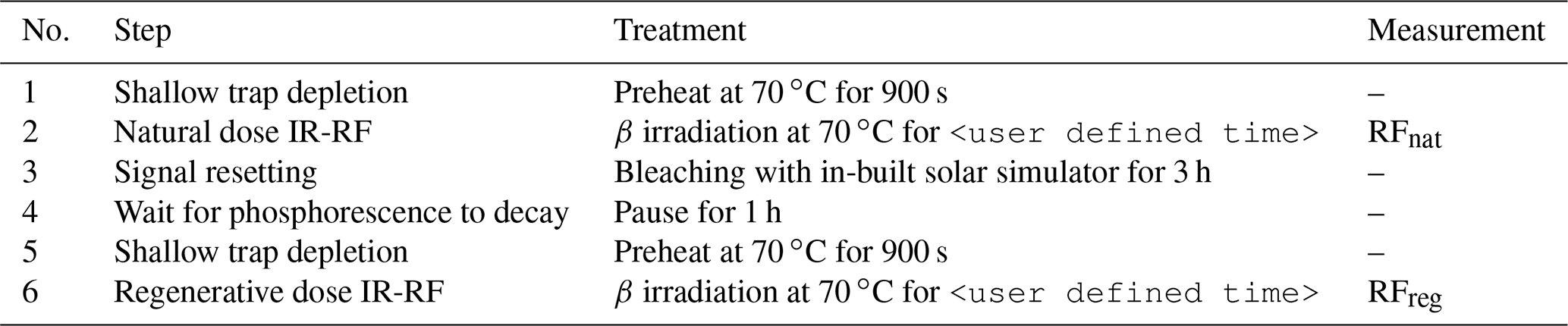
We applied the RF70 single aliquot protocol by Frouin et al. (2017), an improved version of the IRSAR protocol (Erfurt and Krbetschek, 2003a). The RF70 sequence (Table 1) includes two IR-RF measurements: one for the natural signal (RFnat) and one for the regenerated signal (RFreg). In the data analysis process, the RFnat signal curve is slid vertically and horizontally along the signal curve until the best match is achieved with the RFreg curve. The horizontal sliding distance is the accumulated dose needed to match the natural RF signal, thus defining the equivalent dose (Murari et al., 2018). Measurement durations are user-defined. However, RFreg should be longer than the sample's expected natural dose. RFnat should not contain fewer than 70 data points (in our case images) to give sufficient statistical confidence when using the sliding method (Frouin et al., 2017, their supplement, proposed at least 40 channels for a resolution of 15 s/channel).
Table 1Applied IR-RF measurement sequence according to the RF70 protocol by Frouin et al. (2017).
We used the comparable solar simulator settings as in Frouin et al. (2017)2: 365 nm: 20 mW cm−2, 462 nm: 61 mW cm−2, 525 nm: 53 mW cm−2, 590 nm: 37 mW cm−2, 623 nm: 112 mW cm−2, 850 nm: 94 mW cm−2. In our bleaching protocol, the UV power settings are doubled in comparison to the recommendations by Frouin et al. (2015). This setting may lead to an unwanted temperature increase in the sample. However, we carefully monitored the temperature as recorded by the thermocouple in the reader's sample arm. We found the temperature stable at 70 ∘C for all measurements (data not shown), indicating that the temperature in the samples was stable.
2.4 Camera settings
While the enhanced LexStudio 2 version automates image acquisition, it does not free the user from parameterising the camera. In the following, we will advise on the most relevant camera settings and their impact on image noise and signal sensitivity. We derive parts of our advice from signal-to-noise ratio (SNR) estimations summarised in Appendix A. Table 2 lists major correlations between CCD camera settings and data quality. Table 3 lists the camera settings we used in our experiments. For more in-depth insights into the scientific CCD camera technology we may refer to Janesick (2001) and the Andor Learning Centre (https://andor.oxinst.com/learning/, last access: 28 March 2021; search for “Andor Academy”).
Table 2Correlation between basic camera settings and data quality. Up arrows: increasing this parameter leads to an increase of, for example, noise, time span and intensity. Down arrow: increasing this parameter leads to a decrease of the corresponding attribute. Right arrow: changed parameter settings do not affect the attribute.
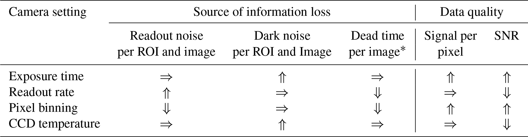
* camera dead time occurs only if a sequential CCD chip readout mode is applied (full-frame mode).
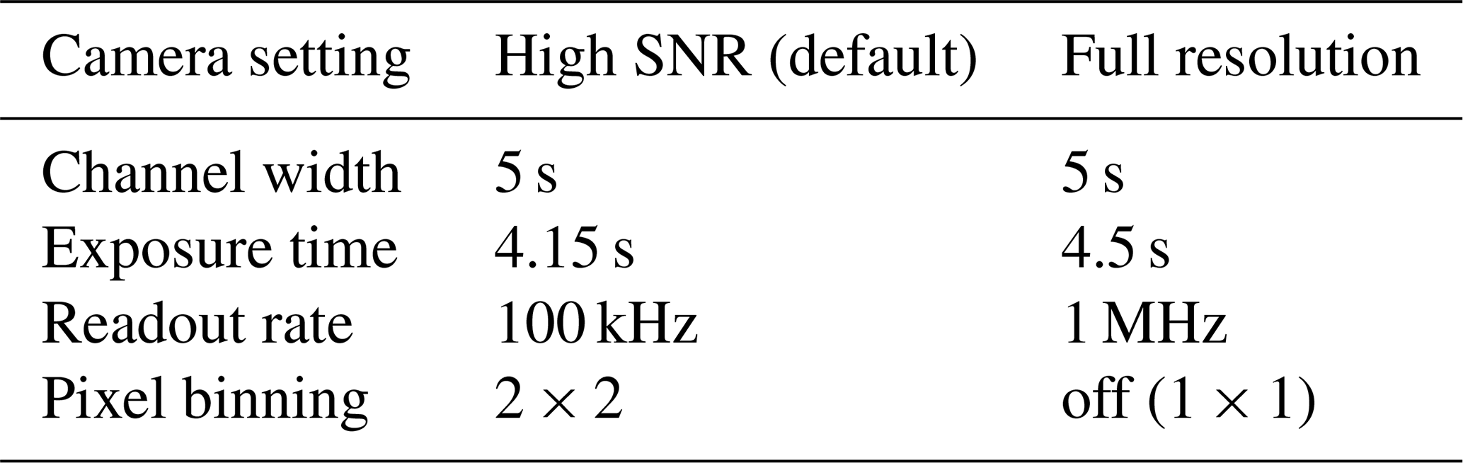
Table 3Recommended settings for a Princeton Instruments ProEM512 camera employed in a Freiberg Instruments lexsyg research system.
2.4.1 Set the CCD chip temperature low, but not too low
One primary source of image noise arises from the dark current of the CCD chip. The dark current is highly temperature-dependent; see Appendix A2 or Fig. S1 for the exact relation. The camera has a built-in thermoelectric cooling system to cool the CCD chip far below room temperature and thus effectively suppressing dark current related image noise. For the camera we used, the lowest reachable CCD temperature is in theory at about −75 ∘C if no additional external cooling is applied. For the user, it seems obvious to set the target CCD temperature as low as the cooling system allows. However, we strongly recommend setting the target temperature between 10 and 15 K above the technical minimum. An RF measurement takes hours, enough time for the camera electronics to warm up or for changes in the system temperature. The resulting fluctuations in the CCD temperature induce changes in the background signal level during the RF measurement. These background instabilities are hard to correct in the post-processing. Therefore, a stationary CCD temperature level is mandatory and eased by leaving the cooling system enough headroom for corrections.
2.4.2 Select a slow readout rate, but not too slow
The CCD chip readout process induces another source of image noise called read noise or readout noise (cf. standard textbooks for both notations). Longer exposure times lead to better SNR because more signal is gathered while the readout noise remains constant.
Another way to reduce readout noise is to choose a slow CCD readout rate. In our system, the slowest available readout rate is 100 kHz. At this rate, a full-resolution (512×512 px) CCD readout takes 2.13 s. If the readout process lasts longer than the RF measurement channel, either images are lost or the camera runs asynchronous to the measurement sequence. In our systems, the readout process started after the preset time interval for the image exposure ended. The camera is then locked until the image data are transferred to the computer. Thus, the user has to incorporate a camera dead time when parameterising channel width and exposure time in the camera's sequence settings; see Table 3 and Appendix A. However, all modern scientific CCD cameras, including our ProEM camera, can read out the last image while already gathering signal light for the next image. The camera dead time is a setting particular to the LexStudio 2 software solution we used. Later software iterations or more advanced systems might set exposure time and channel width equal by default.
2.4.3 Do not use EM gain
EM-CCD cameras have an electron-multiplying (EM) register that amplifies the detected signals above readout noise if activated. The EM mode allows for highly sensitive high-frame-rate imaging, but it comes at a cost: (1) it induces an additional source of image noise (excess noise), (2) it reduces the dynamic range and the linearity of the signal acquisition, (3) it amplifies dark current signals and thus dark noise, and (4) it amplifies local pixel over-exposures leading to pixel-well overflows. Especially the last point is problematic for RF imaging. If the speckle noise caused by bremsstrahlung gets amplified by the EM mode, streaks with increased signal values appear on the image. These are hard to remove by image-processing algorithms.
2.4.4 Consider hardware pixel binning
The most straightforward approach to improving the SNR and the signal sensitivity is pixel binning performed by the CCD camera image-processing software like ImageJ. This software pixel binning, however, is less effective than potential hardware binning by the camera. With applied hardware pixel binning, multiple pixels are considered as one pixel and read out together. This feature reduces the readout noise per imaged area and reduces the readout time and therefore the camera dead time (if applicable). As a side effect, the image stacks' file size is also reduced, positively impacting image processing time. We applied 2×2 pixel binning as a default setting and deactivated it only if we had sufficiently bright samples. On the downside, pixel binning lowers the camera resolution to 256×256 pixel, corresponding to a decreased spatial resolution of 54 µm (before 27 µm).
2.5 Image processing
We obtain two image stacks (a series of images) per aliquot from the RF70 protocol.
(Table 1). Each image stack is
saved as a *.tif file. Both image stacks are affected by speckle noise.
Besides, the RFreg images might be displaced or rotated compared
to the RFnat images due to uncertainties in the aliquot
positioning (Kreutzer et al., 2017).
Both issues and the grain identification are addressed by the SR-RF
macro in ImageJ. The image processing has four steps (Fig. 3): (1) speckle noise is removed, (2) both image stacks are
geometrically aligned, (3) individual grains are identified, and (4)
single-grain RF curves are extracted. Table 4 gives
recommendations for the macro settings. For more details on the macro
settings and the detailed sequence of ImageJ commands, we refer
to our SR-RF macro documentation available at
https://luminescence.de/ (last access: 28 March 2021).
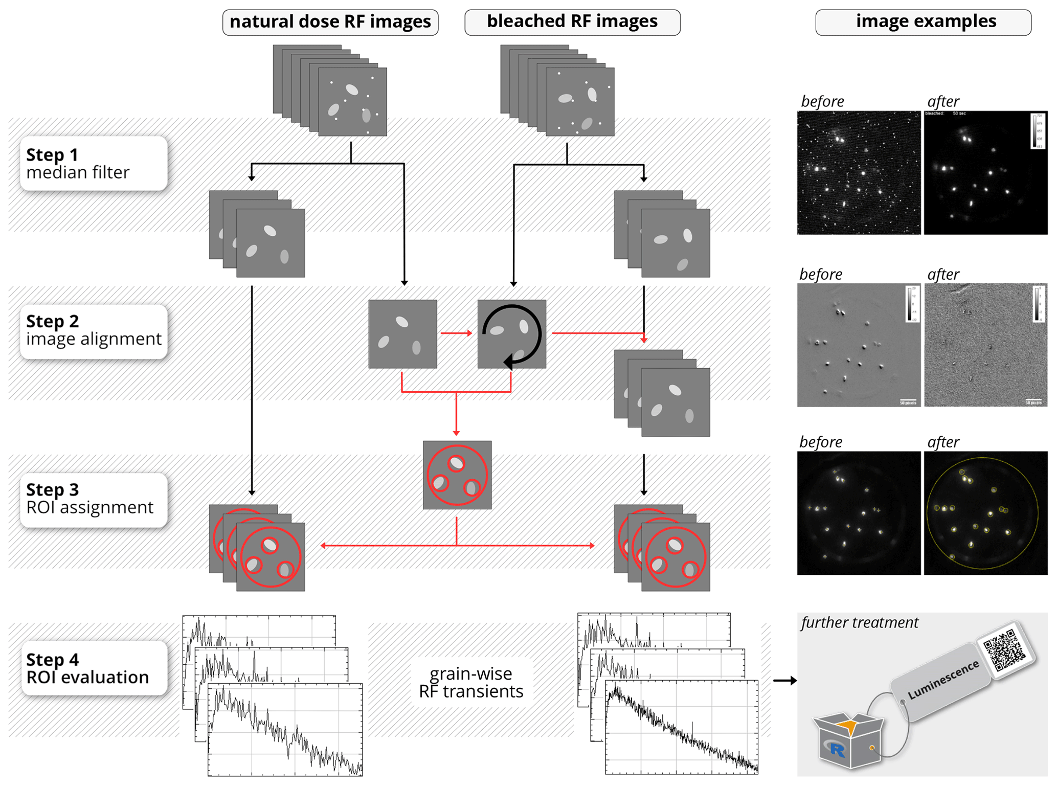
Figure 3Image-processing workflow as performed by the ImageJ macro SR-RF.ijm. Note: the grey step 2 images show the signal value differences between the median signal values of the natural dose RF images and the median signal values of the regenerated dose RF images. A homogeneous colour means that the images are aligned.
Table 4Recommended SR-RF macro settings for the first image-processing run, depending on the sample brightness and the grain size. Parameter refinements depending on the system and the sample might be necessary. The two lower columns display the properties of the resulting single-grain IR-RF curves. The sample area diameter values assume a lateral magnification of 0.6 and a pixel size of 16 µm.
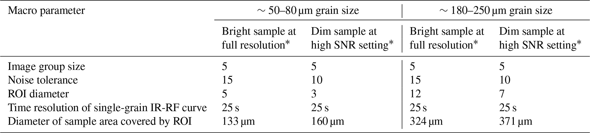
* refers to the recommended camera settings in Table 3.
2.5.1 Step 1: median filter
We used the ImageJ command Grouped Z Project
(Ferreira and Rasband, 2012) to erase bremsstrahlung's spots. The images
of both image stacks are grouped in quantities according to the
user-defined parameter Group Size. Each group's images
are combined to one image by taking the median pixel value for each
pixel location. This process removes signal outliers while maintaining
the fundamental shape of the signal curve
(Velleman, 1980). Speckles caused by bremsstrahlung
occur in random locations. Hence, it is unlikely that the same pixel is
affected more than once during a time interval related to the
measurement of just a few images. The statistical likelihood of
surviving speckles increases with longer image exposure times but
decreases with larger group sizes. For the measurement system we used,
and with an exposure time of 5 s, a group size of five is
sufficient to eradicate speckle noise.
2.5.2 Step 2: image alignment
We used the ImageJ plug-in TurboReg by
Thévenaz et al. (1998) to detect and correct aliquot movement. It
is the same algorithm used by Greilich et al. (2015). The
RFnat and the RFreg stack are aligned by comparing their
global median images. Equal to other regression algorithms, the
differences between median images are summed up to one residual value.
The RFreg median image is rotated and translated until the
minimum is found. The rotation and translation parameters are then
applied to all images of the RFreg stack.
To interpolate the signals for the fine movement of the alignment,
ImageJ offers three methods: none, bilinear and
bicubic (Ferreira and Rasband, 2012). We tested the
interpolation methods for sample TH0 (see below, Sect. 3.4.1)
and selected bicubic as a hidden preset value.
2.5.3 Step 3: grain detection and ROI assignment
We used the ImageJ command Find Maxima
(Ferreira and Rasband, 2012) to identify individual mineral grains, as
a reference serves the arithmetic mean image of the two median
images from step 2 (Sect. 2.5.2). There, the
Find maxima algorithm searches for local maxima in the
pixel values. The user-defined parameter
Noise tolerance controls the algorithm's sensitivity,
which defines how much higher than the surrounding area a pixel value
must be. A higher Noise tolerance value leads to higher
robustness against optical reflections and signal outliers but a lower
grain detection likelihood. A circular ROI is assigned to each local
maximum. The diameter of these circles is user-defined through the
ROI diameter parameter.
2.5.4 Step 4: extract single RF curves
We used the ImageJ ROI manager to obtain the arithmetic
mean of the pixel values in each ROI for each image in the RFnat
stack and RFreg stack. Thus, the consecutive average signal in
one ROI forms the IR-RF curve of one sample grain. These single-grain
IR-RF measurements and the lateral position of each ROI are saved into
one ASCII text file (table.rf) to be further analysed with
other software than ImageJ.
2.6 Single-grain data analysis in R
We analysed the single-grain IR-RF data the same way that we would
analyse conventional PMT IR-RF measurements. A simple R script to
analyse the table.rf file of one aliquot reads as follows (R
package Luminescence ≥ v0.9.8 needed):
#load R package 'Luminescence'
library(Luminescence)

#import data
file <- file.choose()
RF_data <- read_RF2R(file)

#get ROI locations (optional)
ROI_data <- plot_ROI(RF_data)

#determine equivalent doses
equivalent_doses <- analyse_IRSAR.RF(
  object = RF_data,
  method = "SLIDE",
  method.control = list(
    vslide_range = "auto",
    correct_onset = FALSE))

#plot dose distribution
plot_AbanicoPlot(equivalent_doses)
Here, the new function read_RF2R() converts the
table.rf file into a list of RLum.Analysis objects.
Each RLum.Analysis object contains the RFnat and
RFreg curves of one ROI. The equivalent dose of each ROI is
calculated by analyse_IRSAR.RF(), which was already introduced
and used by Frouin et al. (2017). The resulting dose
distribution can be displayed and further evaluated by any of the
various functions for dose statistics the Luminescence package
provides. In the example above, we allowed vertical sliding after
Murari et al. (2018) in the function analyse_IRSAR.RF()
(parameter vslide_range). Vertical sliding can improve the
equivalent dose results' accuracy but needs a significant curvature in
the IR-RF decay to work properly. Vertical sliding can be deactivated by
setting vslide_range = NULL or removing the parameter. The
function plot_ROI() displays and returns the ROI locations and
returns the Euclidean distance between them. This information is useful
to study the impact of signal cross-talk.
2.7 Signal cross-talk
An issue in OSL and TL imaging flagged by Gribenski et al. (2015) and further discussed by Cunningham and Clark-Balzan (2017) is signal cross-talk. Two independent effects cause signal cross-talk: (1) signal light misdirected by optical aberrations and (2) signal light backscattered by the silicone fixation layers and the sample carrier's surface. The visual perceptions are blurry luminescence images and signal halos around individual grains. These halos can extend into the ROIs of other grains located nearby. This cross-talk effect blends the IR-RF curves and potentially narrows the De distribution.
Gribenski et al. (2015) investigated the effects of signal-cross talk in spatially resolved OSL measurements. They found a substantial effect on the equivalent dose outcome and supposed optical aberrations as the primary signal cross-talk source. Like us, they used a lexsyg research device equipped with a ProEM512B camera. However, they measured at the OSL/TL sample position equipped with a custom-made multi-purpose optic (Richter et al., 2013; Greilich et al., 2015). The OSL/TL optic was designed with large opening angles and high UV-to-NIR transmittance. This design decision enabled a maximum of signal yield for various applications but counteracted the optical correction of spherical and chromatic aberration and their secondary effects like astigmatism.
The optic of the RF position has a far smaller aperture (NARF≈0.2 vs. NA) and therefore less spherical aberration. In addition, we consider chromatic aberration as negligible because we performed the focus calibration and all measurements at the same wavelength (865 nm). As Fig. 4 shows, the effect of signal cross-talk appears to be weaker in our measurements as observed by Gribenski et al. (2015) and should be insignificant for inter-grain distances above ca. 500 µm. We tried to maintain this distance by preparing our samples with a very low grain density.
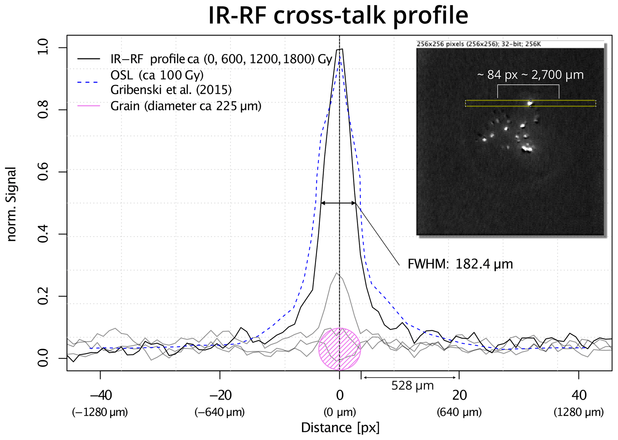
Figure 4IR-RF cross-talk profile of one single grain. The inset shows the ImageJ image with the rectangle area selected for the profiling over ca. 1800 Gy (along the all image slices of the image stack). The solid black lines show the IR-RF signal. For illustrative reasons, we show only a few curves. The dashed blue line shows the approximated OSL cross-talk profile recorded by Gribenski et al. (2015) after a dose of ca. 100 Gy. The violet shaded area approximates the grain (not in height but width). Please note that the data by Gribenski et al. (2015) were only added to provide a rough qualitative comparison. Please note that the metric distances (sub-labels) refer to the chip surface.
Nevertheless, for samples with a high grain density or a high grain intensity inhomogeneity, signal cross-talk will be an issue. We propose the following countermeasures to reduce the effect; none of them applied in our experiments though:
-
Use special sample carriers (punched, black or polished) to minimise backscattered luminescence light.
-
Deploy improved optics (the lenses are exchangeable) to further reduce spherical aberration.
-
Apply mathematical correction methods (e.g. Cunningham and Clark-Balzan, 2017) to improve the grain separation in the data.
3.1 Samples
We selected two potassium-bearing (K-feldspar) samples to apply and test our SR IR-RF tools and their settings. The first sample (TH0, grain size: 125–250 µm) is a modern analogue sample of aeolian origin from Sebkha Tah in Morocco (cf. Bouab, 2005). It is the same sample used by Frouin et al. (2017) to calibrate the 90Sr 90Y source of the very same reader used for our measurements here. The sample was exposed to a γ dose of 56.02 Gy (cv∼2 %) in 2015 (Frouin et al., 2017). The second K-feldspar sample (BDX16651, grain size: 100–200 µm) originates from a coastal dune in the Médoc area (south-western France). For this sample, Kreutzer et al. (2018) estimated a palaeodose of 50.7±5.7 Gy for the quartz fraction (green OSL) and 96.2±8.0 Gy (with IR-RF) for the K-feldspar fraction measured here. For details on the sample preparation procedures, we refer to the cited literature.
3.2 Experiments
TH0 allowed us to calibrate the 90Sr 90Y source with SR IR-RF and compare the results with the PMT's calibration measurements. For this experiment, the detector changed in alternating turns; i.e. after measuring an aliquot with the PMT, another aliquot was measured using the EM-CCD camera, and then we measured an aliquot again with the PMT, and so on. We tested whether both measurements estimate statistically indistinguishable source dose rates.
The measurements of BDX16651 aimed at one main application of single-grain measurements: differentiation between grain fractions with different bleaching history. Kreutzer et al. (2018) reported an age of 37.0±4.9 ka (arithmetic average ± standard deviation) for the feldspar fraction (measured with IR-RF) and 26.1±3.5 ka for the quartz fraction (measured with green OSL). While both ages overlap within 2σ, Kreutzer et al. (2018) reported consistently older ages for the feldspar fraction compared to the quartz fraction for all samples from the site. Therefore, they argued that the natural bleaching was likely insufficient to reset the IR-RF signal of the feldspar grains. SR IR-RF should confirm the quartz result obtained by Kreutzer et al. (2018) and potentially enable us to identify those grains that received a full signal resetting before the last burial.
For both samples, feldspar grains were dispersed randomly on stainless-steel cups aiming at a low grain density. The sample cups were sprayed with a thin layer of silicon oil. However, no mask or other aid was used because this reflects a more realistic aliquot preparation procedure in most laboratories. We aimed at 30 to 50 grains per aliquot. We prepared at least three cups per sample. Irradiation times were equal to values reported in Frouin et al. (2017) and Kreutzer et al. (2018): 3600 s (RFnat) and 30 000 s (RFreg) for sample TH0; 3600 s and 10 000 s for sample BDX16651.
Figure 5 shows typical IR-RF curves from one ROI (in our case one grain) for TH0 (Fig. 5a) and BDX16651 (Fig. 5b). To obtain the Des, we applied the vertical and horizontal sliding technique (Murari et al., 2018) to TH0. The vertical sliding ensures that both curves (RFnat and RFreg) match best based on their shape. This approach was first used by Kreutzer et al. (2017) to corrected for changed signal intensities due to geometry issues. Still, it can also be used to correct sensitivity changes (Murari et al., 2018). For sample BDX16651, only horizontal sliding was used due to the absence of visible curvature in the IR-RF curve.
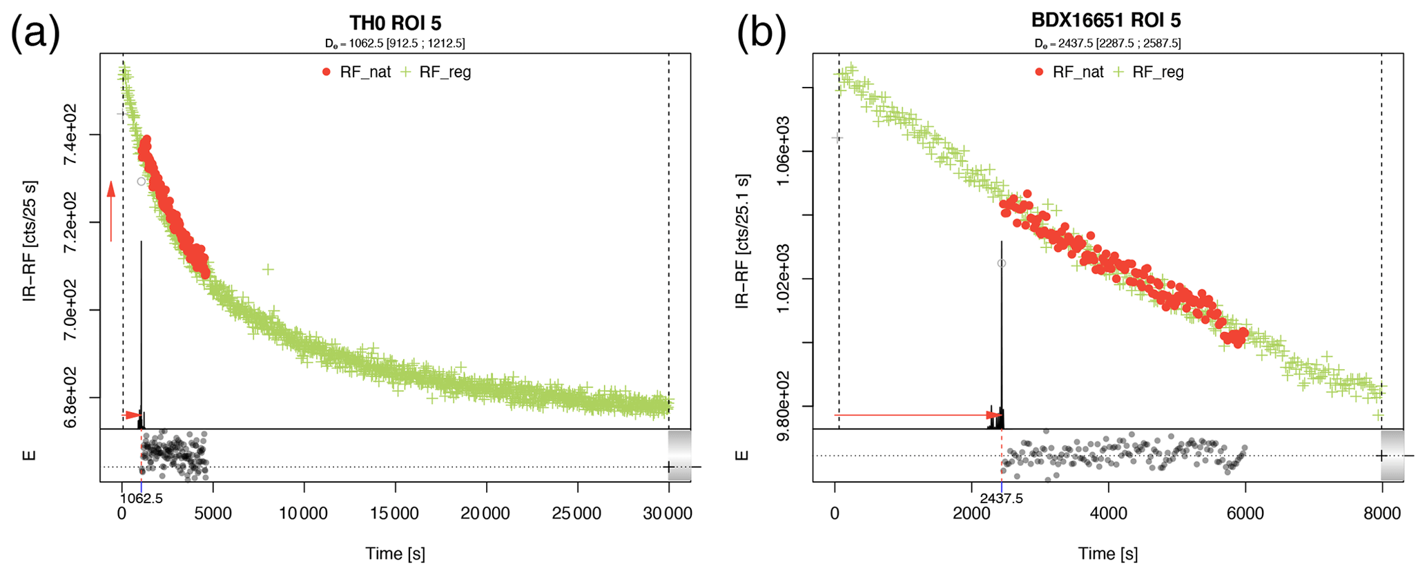
Figure 5Typical IR-RF curves for the samples TH0 (a) and BDX16651 (b). Both curves were extracted from ROIs following the procedure outlined in the first part of the article. For determining the De the sliding method was used. Due to the absence of any curvature in the observed dose range, no vertical sliding was applied to sample BDX16651 measurements (b). Please note, for sample BDX16651 only the first 8000 s of the RFreg are displayed in the figure due to a technical error. SR-RF macro settings as follows: image group size: 5, noise tolerance: 20 (TH0), 30 (BDX16651), grain diameter: 7 px.
As rejection criteria, we applied the default test criteria
(cf. Frouin et al., 2017, their supplement) of the function
analyse_IRSAR.RF(). Two of those criteria were of relevance
for our contribution: curves_ratio and
curves_bounds. The first calculates the ratio of RFnat
over RFreg in the range of RFnat. If it exceeds a certain
threshold (here 1.001), it usually indicates that the RFnat best
matched the RFnat while lying above the RFreg
(additionally confirmed by visual inspection), violating the assumption
that the highest IR-RF signal is observed for the RFreg after
bleaching. If the second, curves_bounds, criterion is flagged,
the RFnat cannot match the RFreg within the measured range
of RFreg – an observation usually made for very noisy, flat
curves.
The raw data of our measurements, along with the applied R scripts and partially pre-processed examples, are available open-access (Kreutzer and Mittelstrass, 2020b).
3.3 Technical camera issues
While we measured at least three cups with grains per sample, the number of usable cups presentable here finally narrowed down to one cup each. A malfunction in the cooling system of our camera stopped us from conducting more measurements. This cooling system degraded over the last 5 years, continually increasing the lowest reachable temperature from at least −70 ∘C in 2015 to about −45 ∘C in 2019. As we already mentioned above, the CCD chip temperature's spatial and temporal uniformity is necessary to ensure a stable and homogeneous signal background. We provide additional insights in Appendix A2 and Figs. S1 and S2 in the Supplement. Unfortunately, our camera's cooling system finally lost its ability to maintain stable chip temperatures during our measurements meant for publication. Significant variations in the IR-RF curves' signal background required us to discard most of our measurements (see Fig. S4 for an example).
Independently from this issue, we further discarded grains located at the rim of the stainless-steel cup, where our analysis indicated exceeded IR-RF curve boundaries for unknown reasons (i.e. no match between RFnat and RFreg).
3.4 Results
Figure 6 illustrates the final results for the two remaining cups: one for TH0 (Fig. 6a, upper part) and one for BDX16651 (Fig. 6b, lower part). For each sample, we show an image taken with the camera (left-hand side) during the measurements and an Abanico plot (Dietze et al., 2016) of the distribution of the results. ROI pixels (diameter 7 px; see Table 4) taken for the De analysis are coloured green and numbered. The numbers are displayed again in the Abanico plots (right-hand side). The results of TH0 display dose rates in Gy s−1 and equivalent doses in Gy for BDX16651. We applied the average dose model (Guérin et al., 2017) to both distributions with an assumed intrinsic overdispersion (σm) of 0.05.

Figure 6The figure shows the SR IR-RF measurement results for single grains from samples TH0 (a) and BDX16651 (b). For each sample, the image of one aliquot with the selected ROIs (green) is plotted on the left-hand side, and the resulting De distribution as Abanico plot (Dietze et al., 2016) on the righthand side. Numbers (white) in the plots identify individual ROIs. The distribution for TH0 shows dose rates and the distribution for BDX16651 equivalent doses. Note: the original images returned by the SR-RF macro have been cropped and reworked in R for this publication.
3.4.1 TH0
SR RF-RF measurements of sample TH0 on 10 grains (ca. 20 grains on the cup, 11 grains emitted sufficient light for the analysis, 1 grain discarded) obtained a source-dose rate of 0.055±0.004 Gy s−1 (date: 13 September 2019). This value is consistent with the source-dose rate calibration value obtained through conventional IR-RF PMT measurements with the same sample (Fig. S5, measurement date: 13 September 2019, n=10, 0.056±0.001 Gy s−1). Hence, it confirms our hypothesis that the calibration results obtained through SR IR-RF and IR-RF PMT measurements are indistinguishable. Furthermore, it gives some confidence that these measurements were not affected by the cooling-system malfunction of the camera.
We further tried to determine to what extent the results depend on
the chosen ROI size (here diameter 7 px) and the interpolation
method used to correct the image for translation and rotation
(Sect. 2.5.2). As an interpolation method, we obtained
the best results for the option bicubic (see Fig. S3), which is
the default in the SR-RF ImageJ macro SR-RF. The ROI
diameter should mimic the approximated grain size or be a bit larger
(see also Fig. S3). We observed a plateau of results for ROI sizes
between 5 and 10 px for sample TH0. Smaller values
should not be selected because the ROI finding algorithm may not
reliably select the grain centre. For larger values, signal cross-talk
effects likely become an issue, although the median appears to be rather
robust for all ROI sizes between 5 and 30 px for
bicubic (Fig. S3).
3.4.2 BDX16651
We counted ca. 40 grains on the analysed cup, and 35 emitted light and
were analysed. We discarded three grains because the R analysis
indicated a bad match of RFnat and RFreg. The sample shows
a large De scatter with an average De of
148.6±6.7 Gy (average dose and associated standard error
(SE)). This value is significantly larger than the mean De of
ca. 96 Gy reported by Kreutzer et al. (2018). However, in
contrast to the study by Kreutzer et al. (2018), the single-grain data
allow further statistical treatment of the results. We applied the
finite mixture model (FMM, cf. Galbraith and Roberts, 2012) using the
function calc_FiniteMixture() with an assumed
sigmab value of 0.05 (Fig. 7). The Bayesian
information criterion indicated the statistically significant number of
components.
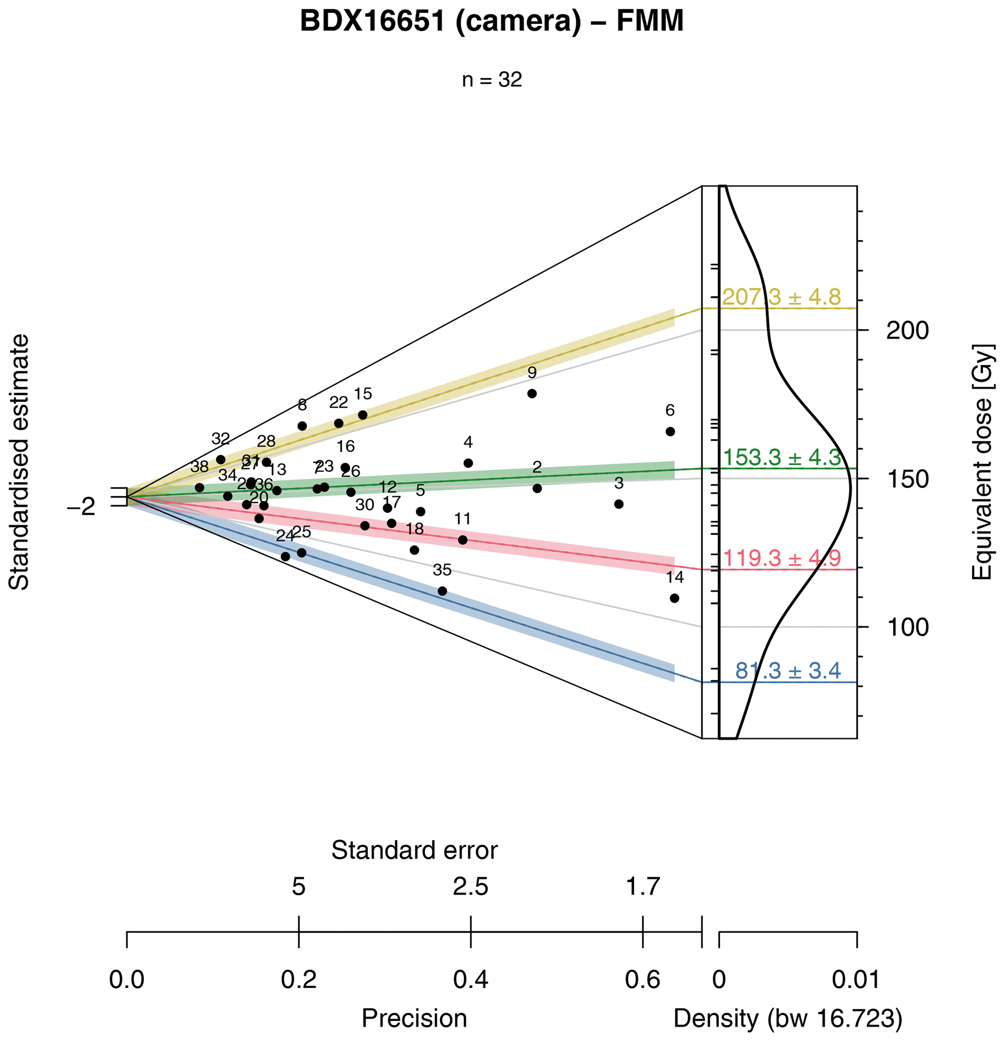
Figure 7Abanico plot for sample BDX16651 with coloured polygons indicating dose components as identified by the finite mixture model. Further details see main text.
We found that four-dose components can best describe the De
distribution. The lowest ca. 81 Gy (blue colour, Fig. 7) contains only 10 % of all grains, the
second component ca. 26 %, the third
ca. 47 % and the highest dose component ca. 19 % of all grains. The number
varies with sigmab (not shown), but the data set seems to
consist of at least two dose groups (around <120 Gy and
>120 Gy). Assuming that the lowest dose group (Fig. 7) corresponds to the best bleached grains (leaving aside
possible layer disturbance and dose rate heterogeneities) the De of
81.3±3.4 Gy corresponds to an IR-RF age of
ca. 31±5 ka, this is more consistent with the quartz age of
26.1±3.5 ka. However, the overall statistical confidence
in ages based on three grains might be doubted, regardless of the
statistically justified number of components. Simultaneously, it appears
that dose groups with higher doses than reported by
Kreutzer et al. (2018) are dominant. Here more measurements would be
needed to infer a statistically robust answer.
We showed that SR-RF is technically feasible and presented first
results. However, some aspects deserve critical consideration.
4.1 The technical dimension
It would be wishful thinking to assume that the work is finished. In comparison to PMT measurements, the number of control parameters exploded similarly to the amount of data. We tried to reduce the complexity by recommending meaningful settings and limit the number of adjustable parameters to a minimum. Still, other systems might have options we did not consider in our contribution.
Besides the technical problem we encountered with the detection chip's cooling system, we also acknowledge that our system is not perfect. A considerable improvement of image quality can be expected from a dedicated RF imaging system. We outline a possible design for such a system in Fig. 8. A system of one or two concave mirrors would allow the relocation of the camera and the filters further away from the β source and thus minimise bremsstrahlung effects and potential filter degradation (cf. Gusarov et al., 2005). Such a mirror optic would also eliminate chromatic aberration and thus enable the ability to take RF images at different wavelengths without refocusing. A dedicated RF optic would also address further optical aberrations and thus reduce signal cross-talk. As a camera, we propose a modern scientific CMOS camera. CMOS cameras have lower readout noise than traditional CCD cameras, although they do not support EM and hardware pixel binning.
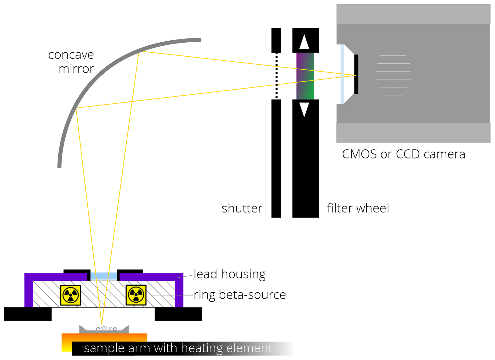
Figure 8Instrumental design proposal for a dedicated SR-RF reader based on a Freiberg Instruments lexsyg research.
Concerning the software, one subject for future improvements we did not implement is an advanced median filter in the image-processing macro. While the current algorithm proved itself powerful in sufficiently removing speckle noise, it decreases the time resolution and deletes those pixel values which are not identified as median values. More sophisticated algorithms deploy complex running median processes. For example, the (53H, twice) algorithm described in Velleman (1980) would mostly maintain time resolution while being still as potent in removing spikes. As another example, the (4253H, twice) algorithm of Velleman (1980) would maintain the shape of the underlying RF curve while smoothing away signal spikes and much of the Gaussian noise.
Another subject of potential improvement is the ROI assignment algorithm. The current algorithm assigns the maximum signal pixel of the grain as the centre of the ROI, no matter if this is the middle of the grain. We suggest a subsequent algorithm which refines the ROI centre towards an estimated grain centre. Consequently, the ROI size could be reduced without losing signal, usually leading to higher inter-aliquot scatter. This would increase grain separation and decrease any influence of signal cross-talk.
Finally, while the presented software toolchain is open-source, hence freely available and open to inspections and improvements, we acknowledge that the combination of three different software tools adds an additional layer of complexity. However, in particular, the image processing through ImageJ has the advantage that the data processing is transparent and available on all platforms and independent of the particular measurement system. Furthermore, users can tap into an extensive repository of available functions and plug-ins to record their own macros and thus adjust the image analysis with ImageJ without a need for programming skills.
4.2 The application dimension
This section alludes to the scientific gain and the initially expressed hypothesis that SR IR-RF can unravel the bleaching history of single feldspar grains.
We showed for sample TH0 that obtained source dose-rate results do not differ significantly from conventional IR-RF results using a PMT. This observation is reassuring because it shows that the presented workflow and analysis leads to meaningful results. However, Fig. 6a also reveals a large scatter between the individual feldspar grains ranging from 0.044 to 0.076 Gy s−1. Richter et al. (2012) reported a variation of the radiation field for our source type of only 2 %. Hence, the extreme values might result from microdosimetric effects (irradiation, cf. Mauz et al., 2020), which are related to IR-RF characteristics of single feldspar grains or varying K concentrations (e.g. Dütsch and Krbetschek, 1997).
Kumar et al. (2020) reported zoning of feldspar grains linked to the geochemical composition. On some of our images (not shown), it appears that the light is not evenly distributed over the grain surface. However, higher optical resolutions would be required to investigate this aspect further.
Sample BDX16651 showed an even higher scatter in the equivalent doses, which is not surprising for a natural sediment sample. While environmental dose rate heterogeneities might add to the observed scatter (Fig. 6b), the internal K concentration of K-feldspar (cf. Huntley and Baril, 1997), in our case contributing ca. 23 % to the environmental dose rate (cf. Kreutzer et al., 2018), weakens the effect. Grain-to-grain variations in the internal K concentrations would undoubtedly broaden the De distribution. However, in our case, the K concentration was sufficiently constrained by energy dispersive X-ray analysis (EDX) (Kreutzer et al., 2018, their Fig. S16) at 11.4±2.5 %3. This value does not have enough leverage to cause results, such as observed for our sample. More important is to keep in mind that IR-RF specifically targets K-feldspar grains, which is amplified by selecting single grains with the highest luminescence intensities and presumed relatively homogeneous K concentrations. Hence, it is more likely that the distribution reflects different bleaching histories with a lower De component (Fig. 7) that gives a luminescence more consistently than the quartz age.
The small number of overall observations, however, does not yet support a more robust conclusion.
Unfortunately, the degraded camera cooling system stopped us from carrying out additional experiments. Does this leave the question open of whether to expect hidden malign effects in the results of samples TH0 and BDX16551? Our observations indicated that cooling system problems were always clearly visible in the IR-RF curves, manifesting in vastly overestimated unrealistic results – an observation we did not make for the presented results.
In the absence of such technical issues, given that our method can be tested successfully at more extensive data sets, the next logical step would be to link SR IR-RF with spectral measurements. Trautmann et al. (2000) performed spectrally resolved radiofluorescence measurements of single feldspar grains. They demonstrated that the radioluminescence emission spectra could significantly differ from grain to grain. They also showed that plagioclase grains might also emit IR-RF signals and mentioned that the separation of K-feldspar grains from other feldspar grains could not be taken for granted. Nevertheless, Trautmann et al. (2000) concluded that “good” grains and “bad” grains might be distinguishable by their spectral fingerprint. In the same year, Krbetschek et al. (2000) showed that artificial irradiation could stimulate an RF emission centred at 700 nm. This additional emission may interfere with IR-RF measurements. However, for the sample BDX16651, we performed brief tests with a spectrometer and did not find any indication for a potential signal interference (not shown, to be presented elsewhere).
Successive spatially resolved RF measurements at different wavelengths are possible if the measurement device deploys an automated filter wheel. In principle, it is even possible to rotate the filter wheel during one measurement and take RF images of multiple wavelengths almost simultaneously. Nevertheless, this would require a significant software update. Still, the software framework presented in this paper may provide the basis to analyse such measurements.
Buylaert et al. (2018) unsuccessfully searched for a correlation between K concentration and the post-IR infrared stimulated luminescence (IRSL) De in single grains of K-feldspar. Recently, Kumar et al. (2020) reported a correlation of the K concentration and the IR signal measured with cathodoluminescence. Spatially resolved RF measurements in combination with spatially resolved IRSL measurements may help to link both observations.
For the first time, we outlined technique and workflow for spatially resolved infrared radiofluorescence (SR IR-RF). We presented the first measurement results and a newly developed open-source software toolchain, applicable independent of manufacturer.
In contrast to routine PMT experiments, spatially resolved measurements come with more degrees of freedom that need to be taken into account, making first steps foremost a technical challenge. Our contribution detailed relevant technical parameters of the imaging system and provided application guidelines. This will allow other laboratories to repeat our work and remove significant obstacles in applying this promising method.
Tests on two K-feldspar samples showed results consistent with IR-RF measurements with a photomultiplier tube (PMT) for the sample TH0. However, our results also showed a large grain-to-grain scatter, requiring more attention and more future measurements. For the sample BDX16651, we identified up to four different De components, with the lowest component resulting in an IR-RF age still older than the corresponding quartz age. This finding may indicate that this particular sample's bleaching time was insufficient to reset the natural IR-RF signal during sediment transport. However, if insufficient resetting has affected all K-feldspar grains, it cannot be resolved by spatially resolved measurements, but it indicates the current limit of IR-RF due to its slower signal bleachability compared to quartz.
We faced several technical issues, foremost the unstable signal background due to a camera defect. This observation demonstrates the higher complexity and potentially more error-prone technical setup than IR-RF measurements with a photomultiplier tube. Nevertheless, we are confident that more measurements using fully functional systems can exploit the presented method's full potential.
A1 Signal per pixel
If the signal shows no unsteadiness, inhomogeneity, non-linearity or any background signal shape, the expected signal per image pixel μpixel (in photoelectrons e−) after background correction approximates to
where ϕpixel is the rate of luminescence-related photoelectrons generated in one CCD pixel in e−/px/s. We assume that ϕpixel depends linearly on the actual photon flux emitted by the sample by an unknown constant. The other parameters are explained and discussed in the following. Be aware that all signal and noise values in the following use the unit photoelectrons per pixel e−, which is not equal to the unit counts per pixel displayed in the image data. The conversion rate between photoelectrons and counts depends on multiple camera settings and is of just minor relevance for the signal-to-noise ratio (SNR) and therefore not discussed here. Be also aware that if not stated otherwise, we always refer to image pixels and not CCD pixels.
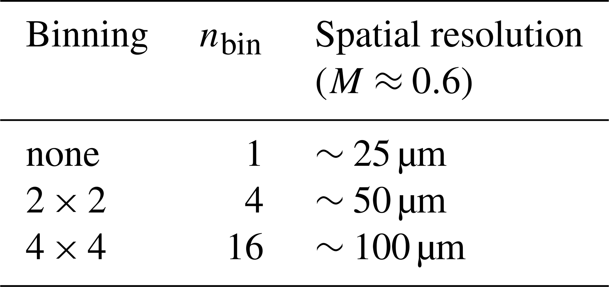
The binning factor nbin expresses the number of CCD pixels combined to one image pixel. Applying pixel binning improves the signal-to-noise ratio, because the signal of the pixels is summed up, but this signal is only affected by readout noise one time. The RF optic of the lexsyg research system has a lateral magnification of about M≈0.6. The resulting spatial resolution is listed in Table A1 (11/2018 @L2, IRAMAT-CRP2A).
Table A1Spatial resolution and binning factor dependent on pixel binning.
The image exposure time texposure (s) is user-defined. It is reasonable to set the exposure time depending on the measurements channel time tchannel (s):
-
sequential readout (full-frame mode):
-
simultaneous readout (frame transfer mode): texposure=tchannel.
If the camera runs in full-frame mode, any luminescence signal and trigger signal arriving during pixel shifting, pixel readout and data transmission will be lost. This is the case for measurements achieved with LexStudio 2 (11/2018 @L2, IRAMAT-CRP2A) and results in a recommended camera dead time tdead (s). Table A2 shows tested and believed safe dead-time values. Within this time range, the camera will have finished image readout and transmission. Shorter dead times may work but likely lead to lost trigger signals and therefore lost images. If the camera runs in frame transfer mode (default mode for most scientific CCD imaging systems), the image shifted into a special readout section on the CCD chip after the exposure time ended. The image can be read out while the new exposure can already begin (simultaneous readout). If the exposure time is longer than the readout time (plus a little offset), no dead time is necessary.
Table A2Left: CCD readout time as returned by the camera software representing theoretical lowest dead time values. Right: experimentally derived upper dead time limits (recommended settings). For the measurement the amplifier was run in low noise mode and we used the default camera settings.

A2 Noise per pixel
For each image pixel, we assume that the signal noise (σpixel) follows a normal distribution resulting from the superimposition of three independent sources:
The shot noise (σshot) is caused by the random arrival of the photons and obeys Poisson statistics (Janesick, 2001). This noise component is independent of any camera parameter setting and only a function of the expected luminescence signal given by the square root of Eq. (A1).
The dark shot noise (σdark) is the shot noise of the dark current of the CCD:
The dark current signal ϕdark is one of two sources of camera-internal signal background (besides the ADC offset, which contributes no significant noise). The dark current arises mainly from thermally released charge carriers at the CCD surface and in the depletion region (Janesick, 2001). The dark shot noise is nearly exponentially dependent on the CCD temperature TCCD (∘C), and its value is characteristic to each individual camera (cf. Janesick, 2001).
As rule of thumb, reducing the CCD chip temperature by 10 K quarters the dark current signal and halves the dark noise. The following estimation formula is derived from the Certificate of Performance dark charge calibration value of our camera (PI ProEM512B @L2, IRAMAT-CRP2A) and multiple specifications sheets of similar cameras:
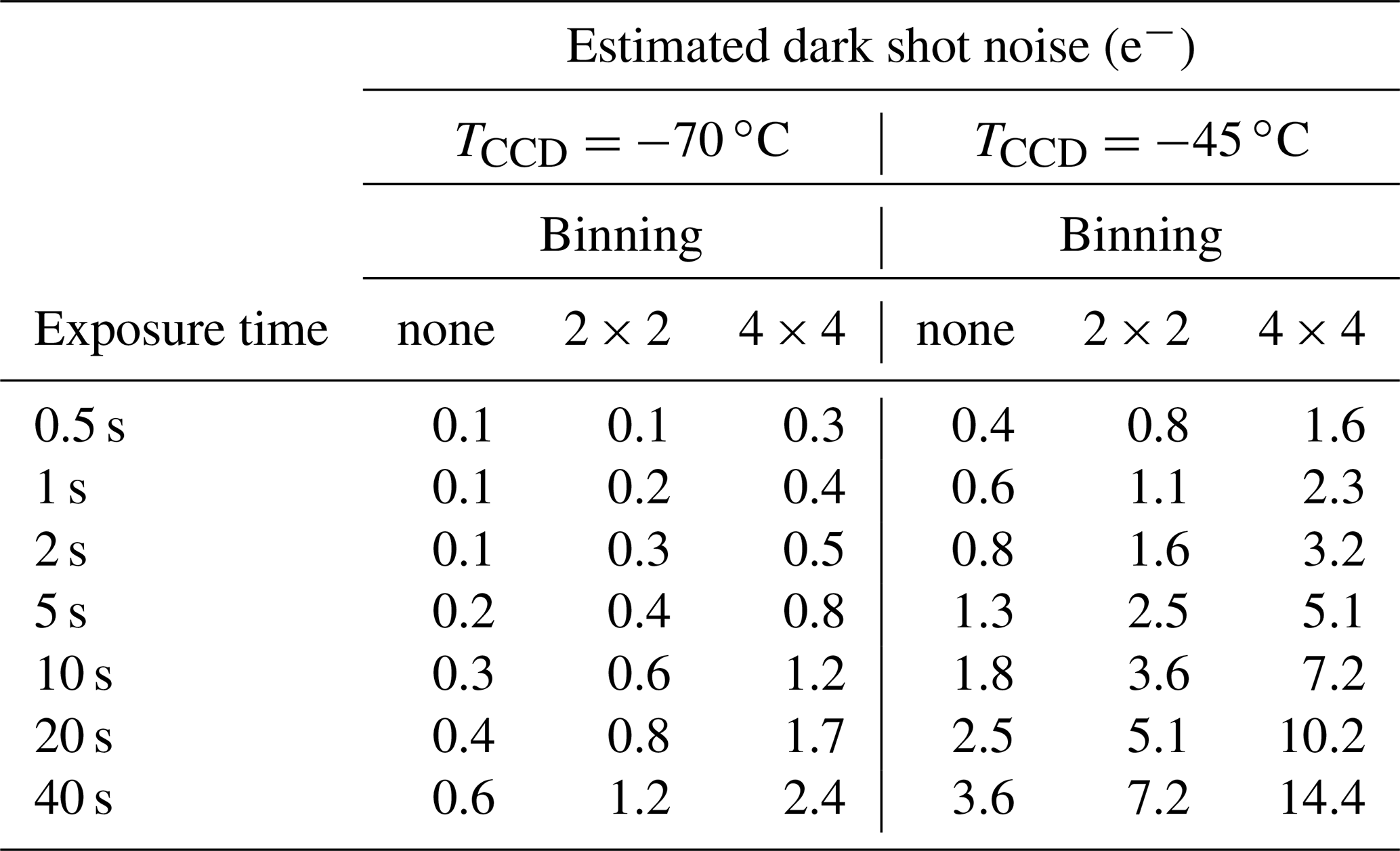
See Fig. S1 in the Supplement for a plot of that equation. The dark current signal itself dissolves in the data analysis process. However, the contribution of the dark shot noise in Eq. (A2) grows with the binning factor, the exposure time and especially the CCD temperature. The dark shot noise of the camera used in this contribution is estimated in Table A3.
Table A3Dark shot noise per image pixel estimation depending on exposure time, binning factor and CCD temperature for an average Princeton Instruments ProEM512 camera.
The readout noise σread is a result of the register readout. It is independent of the exposure time and the CCD temperature and approximately independent from pixel binning. The readout noise increases with increasing readout rate. For our camera and deploying the available traditional amplifier readout modes, readout noise values are listed in Table A4.
Table A4Readout noise dependence of readout rate using the traditional low noise amplifier. Values according to the Certificate of Performance of the PI ProEM512B camera at device L2, IRAMAT-CRP2A.
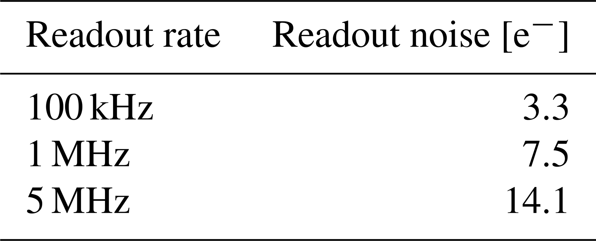
Scientific CCD cameras of this type achieve usually a readout noise of ∼3 e− at 100 kHz and ∼5 e− at 1 MHz (as for 2018).
The signal-to-noise ratio (SNR) is a common quality marker for measurement data. The SNR per image pixel is defined by
Approximations of the signal per pixel μpixel and the noise per pixel σpixel are given by Eqs. (A1) and (A2).
A3 Signal-to-noise ratio per grain
In terms of image processing, a grain is defined by its region of interest (ROI). While the pixel SNR (Eq. A5) can help to optimise the camera settings, it does not factor the size of the ROI in. It is reasonable to set the ROI diameter about 50 % larger than the average grain diameter. With the lateral magnification known (here M=0.6) and the CCD pixel size known (here dpixel=16 µm), the grain size can be converted into pixels and vice versa.
To approximate the SNR of a single-grain IR-RF signal dependent on the ROI size, we assume that the signal remains on a steady level (no decay) and that all signal light reaching the CCD is gathered in the associated ROI (no light scattering). Then, the IR-RF signal per grain (μgrain) depends just on the emitted photon flux of the grain and the exposure time texposure.
Here, ϕgrain is the signal flux per grain (in e−/s) inside the ROI, which is proportional to the emitted photon flux. The signal per pixel μpixel (Eq. A1) for all ROI pixels adds up to the signal per grain μgrain. We consider the distribution of μpixel inside the ROI as unimportant.
While the grain signal μgrain is independent on all parameters but the exposure time, the signal noise per grain σgrain depends also on the ROI size nROI and the camera settings:
Thus, the single-grain radiofluorescence signal-to-noise ratio SNRgrain can be approximated by
Here, nROI is the number of pixels in the ROI, available in the
table.rf file. The signal per grain ϕgrain has to be
user-defined and can be considered as the same order of magnitude as the
counts per second a grain would contribute to PMT measurements. We
defined an arbitrary dim grain and estimated SNRgrain for
different camera settings in Table A5. We consider a SNR
of at least SNRgrain>3 as necessary to enable sufficiently
precise single-grain dating.
Table A5Decision table for best binning and channel time settings. We compare the system used in our study and a (hypothetical) similar system with comparable new camera and improved control software. Bold SNR values are related to the high SNR camera settings, recommend in Table 3.
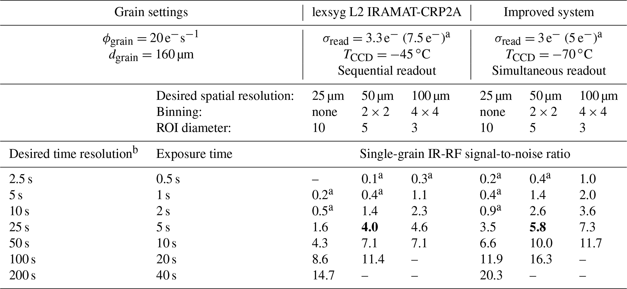
a Readout rate of 1 MHz necessary to account for short exposure times. Values without superscript apply a default readout rate of 100 kHz;
b Time resolution of the processed image stack, given a image group size of n=5 is parameterised.
The SR-RF macro developed for this paper and used for
image processing and the software toolchain overview and tutorials
are available at http://doi.org/10.5281/zenodo.4745491 (Mittelstraß and Kreutzer, 2021). The R package
RLumSTARR used for an automated data processing is available at
https://github.com/R-Lum/RLumSTARR (Kreutzer and Mittelstrass, 2020a). The SR-RF macro and RLumSTARR are
distributed under GPL-3 licence conditions. The
data sets presented in this paper as well as the used measurement sequences and analysis scripts
are available at https://doi.org/10.5281/zenodo.4395968 (Kreutzer and Mittelstrass, 2020b) and make use of
the Creative Commons License
(CC-BY-NC).
Please contact Dirk Mittelstraß (dirk.mittelstrass@luminescence.de) for technical questions and Sebastian Kreutzer (sebastian.kreutzer@aber.ac.uk) for questions on the experiments.
The supplement related to this article is available online at: https://doi.org/10.5194/gchron-3-299-2021-supplement.
DM developed the ImageJ image-processing algorithm and investigated the image acquisition issue. SK performed the measurements, provided the interface to R and investigated the signal cross-talk issue. Both authors helped Freiberg Instruments to solve technical issues. Both authors jointly analysed the data and contributed equally to the article.
The last upgrade of the IR-RF measurement system in Bordeaux was financially supported by the Freiberg Instruments GmbH. However, the manufacturer had no part in the scientific work or this article. The authors declare no further competing interests.
The authors developed the attached and linked software tools with great care and the reader may find them useful. However, the software comes without any warranty, without even the implied warranty of merchantability or fitness for a particular purpose.
We are grateful to three anonymous reviewers and James K. Feathers for
constructive and supportive comments. Camille Moreau is thanked for her
work in the framework of her internship at the IRAMAT-CRP2A in 2018.
Ingrid Stein and Detlev Degering are thanked for safeguarding long
forgotten data treasures. Chantal Tribolo and Norbert Mercier are
thanked for fruitful discussions and tremendous patience while waiting
for this article. The authors thank Freiberg Instruments GmbH for
their support and for suffering the noise we made. Finally, we thank
Daniel Nüst for creating and maintaining this wonderful Copernicus
markdown template shipped with rticles (Allaire et al., 2021), which made
compiling this article a lot easier. This work received financial
support from LaScArBx LabEx, a programme supported by the ANR –
no. ANR-10-LABX-52. In 2020, while the data analysis and the
article were completed. Sebastian Kreutzer has received funding from the European
Union's Horizon 2020 research and innovation programme under the Marie
Skłodowska-Curie grant agreement no. 844457 (CREDit). Dirk Mittelstraß took this
research as private endeavour and did not receive any specific grant from
funding agencies in the public, commercial or not-for-profit sectors.
This research has been supported by the European Union's Horizon 2020 research and innovation programme under the Marie Skłodowska-Curie grant agreement no. 844457 (CREDit) and the Agence Nationale de la Recherche (grant no. ANR-10-LABX-52).
This paper was edited by James Feathers and reviewed by three anonymous referees.
Allaire, J. J., Xie, Y., R Foundation, Wickham, H., Journal of Statistical Software, Vaidyanathan, R., Association for Computing Machinery, Boettiger, C., Elsevier, Broman, K., Mueller, K., Quast, B., Pruim, R., Marwick, B., Wickham, C., Keyes, O., Yu, M., Emaasit, D., Onkelinx, T., Gasparini, A., Desautels, M.-A., Leutnant, D., MDPI, Taylor and Francis, Öğreden, O., Hance, D., Nüst, D., Uvesten, P., Campitelli, E., Muschelli, J., Hayes, A., Kamvar, Z. N., Ross, N., Cannoodt, R., Luguern, D., Kaplan, D. M., Kreutzer, S., Wang, S., Hesselberth, J., and Dervieux, C.: rticles: Article Formats for R Markdown, R package version 0.18.3, available at: https://CRAN.R-project.org/package=rticles (last access: 28 March 2021), GitHub, 2021. a
Baril, M. R.: CCD imaging of the infra-red stimulated luminescence of feldspars, Radiat. Meas., 38, 81–86, https://doi.org/10.1016/j.radmeas.2003.08.005, 2004. a
Bortolot, V. J.: A new modular high capacity OSL reader system, Radiat. Meas., 32, 751–757, https://doi.org/10.1016/S1350-4487(00)00038-X, 2000. a
Bøtter-Jensen, L., Bulur, E., Duller, G. A. T., and Murray, A. S.: Advances in luminescence instrument systems, Radiat. Meas., 32, 523–528, https://doi.org/10.1016/S1350-4487(00)00039-1, 2000. a
Bøtter-Jensen, L., Andersen, C. E., Duller, G. A. T., and Murray, A. S.: Developments in radiation, stimulation and oberservation facilities in luminescence measurements, Radiat. Meas., 37, 535–541, https://doi.org/10.1016/S1350-4487(03)00020-9, 2003. a
Bouab, N.: Application Des Methodes de Datation Par Luminescence Optique À L'évolution Des Environnements Désertiques – Sahara Occidental (Maroc) Et Iles Canaries Orientales (Espagne) , Ph.D. thesis, Université du Québec à Montréal, Canada, available at: http://constellation.uqac.ca/868/1/13721974.pdf (last access: 28 March 2021), 2005. a
Buylaert, J. P., Újvári, G., Murray, A. S., Smedley, R. K., and Kook, M.: On the relationship between K concentration, grain size and dose in feldspar, Radiat. Meas., 120, 181–187, https://doi.org/10.1016/j.radmeas.2018.06.003, 2018. a
Chauhan, N., Adhyaru, P., Vaghela, H., and Singhvi, A. K.: EMCCD based luminescence imaging system for spatially resolved geo-chronometric and radiation dosimetric applications, J. Instrum., 9, P11016, https://doi.org/10.1088/1748-0221/9/11/P11016, 2014. a
Clark-Balzan, L. and Schwenninger, J.-L.: First steps toward spatially resolved OSL dating with electron multiplying charge-coupled devices (EMCCDs): System design and image analysis, Radiat. Meas., 47, 797–802, https://doi.org/10.1016/j.radmeas.2012.01.018, 2012. a
Cunningham, A. and Clark-Balzan, L.: Overcoming crosstalk in luminescence images of mineral grains, Radiat. Meas., 106, 498–505, https://doi.org/10.1016/j.radmeas.2017.06.004, 2017. a, b, c
Dietze, M., Kreutzer, S., Burow, C., Fuchs, M. C., Fischer, M., and Schmidt, C.: The abanico plot: visualising chronometric data with individual standard errors, Quat. Geochronol., 31, 12–18, https://doi.org/10.1016/j.quageo.2015.09.003, 2016. a, b
Duller, G. A. T. and Roberts, H. M.: Seeing Snails in a New Light, Elements, 14, 39–43, https://doi.org/10.2138/gselements.14.1.39, 2018. a
Duller, G. A. T., Bøtter-Jensen, L., and Markey, B. G.: A luminescence imaging system based on a CCD camera, Radiat. Meas., 27, 91–99, https://doi.org/10.1016/S1350-4487(96)00120-5, 1997. a
Duller, G. A. T., Kook, M., Stirling, R. J., Roberts, H. M., and Murray, A. S.: Spatially-resolved thermoluminescence from snail opercula using an EMCCD, Radiat. Meas., 81, 157–162, https://doi.org/10.1016/j.radmeas.2015.01.014, 2015. a
Duller, G. A. T., Gunn, M., and Roberts, H. M.: Single grain infrared photoluminescence (IRPL) measurements of feldspars for dating, Radiat. Meas., 133, 106313, https://doi.org/10.1016/j.radmeas.2020.106313, 2020. a
Dütsch, C. and Krbetschek, M. R.: New methods for a better internal 40K dose rate determination, Radiat. Meas., 27, 377–381, https://doi.org/10.1016/S1350-4487(96)00153-9, 1997. a
Erfurt, G. and Krbetschek, M.: IRSAR – A single-aliquot regenerative-dose dating protocol applied to the infrared radiofluorescence (IR-RF) of coarse-grain K-feldspar, Ancient TL, 21, 35–42, 2003a. a, b
Erfurt, G. and Krbetschek, M. R.: Studies on the physics of the infrared radioluminescence of potassium feldspar and on the methodology of its application to sediment dating, Radiat. Meas., 37, 505–510, https://doi.org/10.1016/S1350-4487(03)00058-1, 2003b. a
Ferreira, T. and Rasband, W.: ImageJ User Guide IJ 1.46r, available at: https://imagej.nih.gov/ij/docs/guide/146.html (last access: 28 March 2021), 2012. a, b, c
Fitzsimmons, K. E.: Applications in Aeolian Environments, in: Handbook of Luminescence Dating, edited by: Bateman, M. D., Whittles Publishing, Dunbeath, Scotland, UK, 110–152, 2019. a
Frouin, M., Huot, S., Mercier, N., Lahaye, C., and Lamothe, M.: The issue of laboratory bleaching in the infrared-radiofluorescence dating method, Radiat. Meas., 81, 212–217, https://doi.org/10.1016/j.radmeas.2014.12.012, 2015. a, b
Frouin, M., Huot, S., Kreutzer, S., Lahaye, C., Lamothe, M., Philippe, A., and Mercier, N.: An improved radiofluorescence single-aliquot regenerative dose protocol for K-feldspars, Quat. Geochronol., 38, 13–24, https://doi.org/10.1016/j.quageo.2016.11.004, 2017. a, b, c, d, e, f, g, h, i, j, k, l, m
Galbraith, R. F. and Roberts, R. G.: Statistical aspects of equivalent dose and error calculation and display in OSL dating: An overview and some recommendations, Quat. Geochronol., 11, 1–27, https://doi.org/10.1016/j.quageo.2012.04.020, 2012. a
Greilich, S., Glasmacher, U. A., and Wagner, G. A.: Spatially resolved detection of luminescence: a unique tool for archaeochronometry, Naturwissenschaften, 89, 371–375, https://doi.org/10.1007/s00114-002-0341-z, 2002. a
Greilich, S., Glasmacher, U. A., and Wagner, G. A.: Optical dating of granitic stone surfaces, Archaeometry, 47, 645–665, https://doi.org/10.1111/j.1475-4754.2005.00224.x, 2005. a
Greilich, S., Harney, H.-L., Woda, C., and Wagner, G. A.: AgesGalore – A software program for evaluating spatially resolved luminescence data, Radiat. Meas., 41, 726–735, https://doi.org/10.1016/j.radmeas.2005.12.007, 2006. a
Greilich, S., Gribenski, N., Mittelstraß, D., Dornich, K., Huot, S., and Preusser, F.: Single-grain dose-distribution measurements by optically stimulated luminescence using an integrated EMCCD-based system, Quat. Geochronol., 29, 70–79, https://doi.org/10.1016/j.quageo.2015.06.009, 2015. a, b, c, d
Gribenski, N., Preusser, F., Greilich, S., Huot, S., and Mittelstraß, D.: Investigation of cross talk in single grain luminescence measurements using an EMCCD camera, Radiat. Meas., 81, 163–170, https://doi.org/10.1016/j.radmeas.2015.01.017, 2015. a, b, c, d, e, f
Guérin, G., Christophe, C., Philippe, A., Murray, A. S., Thomsen, K. J., Tribolo, C., Urbanova, P., Jain, M., Guibert, P., Mercier, N., Kreutzer, S., and Lahaye, C.: Absorbed dose, equivalent dose, measured dose rates, and implications for OSL age estimates: Introducing the Average Dose Model, Quat. Geochronol., 41, 163–173, https://doi.org/10.1016/j.quageo.2017.04.002, 2017. a
Gusarov, A., Doyle, D., Glebov, L., and Berghmans, F.: Comparison of radiation-induced transmission degradation of borosilicate crown optical glass from four different manufacturers, in: Optics & Photonics 2005, edited by: Taylor, E. W., SPIE, 5897, 58970I1-8, https://doi.org/10.1117/12.619199, 2005. a
Huntley, D. J. and Baril, M. R.: The K content of the K-feldspars being measured in optical dating or in the thermoluminescence dating, Ancient TL, 15, 11–13, available at: http://ancienttl.org/ATL_15-1_1997/ATL_15-1_Huntley_p11-13.pdf (last access: 28 March 2021), 1997. a
Huntley, D. J. and Kirkley, J. J.: The use of an image intensifier to study the TL intensity variability of individual grains, 3, 1–4, available at: http://ancienttl.org/ATL_03-2_1985/ATL_03-2_Huntley_p1-4.pdf (last access: 4 May 2021), 1985. a
Huntley, D. J., Godfrey-Smith, D. I., and Thewalt, M. L. W.: Optical dating of sediments, Nature, 313, 105–107, https://doi.org/10.1038/313105a0, 1985. a
Janesick, J. R.: Scientific charge-coupled devices, SPIE Press Book, SPIE Press, Bellingham, United states, 907 pp., https://doi.org/10.1117/3.374903, 2001. a, b, c, d
Kook, M., Lapp, T., Murray, A., Thomsen, K., and Jain, M.: A luminescence imaging system for the routine measurement of single-grain OSL dose distributions, Radiat. Meas., 81, 171–177, https://doi.org/10.1016/j.radmeas.2015.02.010, 2015. a
Krbetschek, M. R. and Degering, D.: Spatially resolved Infrared– Radiofluorescence (IR-RF) Dating – on single feldpar grains, in: 11th International LED Cologne, Oral presentation, Cologne, Germany, 1–24, 2005. a, b
Krbetschek, M. R., Trautmann, T., Dietrich, A., and Stolz, W.: Radioluminescence dating of sediments: methodological aspects, Radiat. Meas., 32, 493–498, https://doi.org/10.1016/S1350-4487(00)00122-0, 2000. a, b
Kreutzer, S. and Mittelstrass, D.: RLumSTARR: Spatially Resolved Radiofluorescence Analysis, R package version 0.1.0.9000-49, available at: https://github.com/R-Lum/RLumSTARR (last access: 28 March 2021), 2020a. a, b
Kreutzer, S. and Mittelstrass, D.: Spatially Resolved Infrared Radiofluorescence (SR IR-RF) Image Data, Zenodo [data set], https://doi.org/10.5281/zenodo.4395968, 2020b. a, b
Kreutzer, S., Schmidt, C., Fuchs, M. C., Dietze, M., Fischer, M., and Fuchs, M.: Introducing an R package for luminescence dating analysis, Ancient TL, 30, 1–8, available at: http://ancienttl.org/ATL_30-1_2012/ATL_30-1_Kreutzer_p1-8.pdf (last access: 28 March 2021), 2012. a
Kreutzer, S., Murari, M. K., Frouin, M., Fuchs, M., and Mercier, N.: Always remain suspicious: a case study on tracking down a technical artefact while measuring IR-RF, Ancient TL, 35, 20–30, available at: http://ancienttl.org/ATL_35-1_2017/ATL_35-1_Kreutzer_p20-30.pdf (last access: 28 March 2021), 2017. a, b, c
Kreutzer, S., Duval, M., Bartz, M., Bertran, P., Bosq, M., Eynaud, F., Verdin, F., and Mercier, N.: Deciphering long-term coastal dynamics using IR-RF and ESR dating: A case study from Médoc, south-West France, Quat. Geochronol., 48, 108–120, https://doi.org/10.1016/j.quageo.2018.09.005, 2018. a, b, c, d, e, f, g, h, i, j, k
Kreutzer, S., Burow, C., Dietze, M., Fuchs, M. C., Schmidt, C., Fischer, M., Friedrich, J., Riedesel, S., Autzen, M., and Mittelstrass, D.: Luminescence: Comprehensive Luminescence Dating Data Analysis, R package version 0.9.9, available at: https://CRAN.R-project.org/package=Luminescence (last access: 28 March 2021), 2020. a
Kumar, R., Martin, L. I. D. J., Poelman, D., Vandenberghe, D., De Grave, J., Kook, M., and Jain, M.: Site-selective mapping of metastable states using electron-beam induced luminescence microscopy, Scientific Reports, 10, 15650, https://doi.org/10.1038/s41598-020-72334-7, 2020. a, b
Liritzis, Y. and Galloway, R. B.: Bremsstrahlung from a shielded beta irradiator, J. Radioanal. Nucl. Ch., 146, 333–345, https://doi.org/10.1007/BF02164236, 1990. a
Maraba, D. and Bulur, E.: Design and construction of an automated OSL reader with open source software and hardware, Radiat. Meas., 106, 632–637, https://doi.org/10.1016/j.radmeas.2017.04.011, 2017. a
Mauz, B., Martin, L., Discher, M., Tribolo, C., Kreutzer, S., Bahl, C., Lang, A., and Mercier, N.: Technical note: On the reliability of laboratory beta-source calibration for luminescence dating, Geochronology Discuss. [preprint], https://doi.org/10.5194/gchron-2020-36, in review, 2020. a
Mittelstraß, D. and Kreutzer, S.: ImageJ macro for spatially resolved infrared radiofluorescence (SR-RF) (Version v0.1.0), Zenodo, https://doi.org/10.5281/zenodo.4745491, 2021. a
Murari, K. M., Kreutzer, S., King, G., Frouin, M., Tsukamoto, S., Schmidt, C., Lauer, T., Klasen, N., Richter, D., Friedrich, J., Mercier, N., and Fuchs, M.: Infrared Radiofluorescence (IR-RF), Quat. Geochronol., 64, 101155, 10.1016/j.quageo.2021.101155, 2021. a
Murari, M. K., Kreutzer, S., and Fuchs, M.: Further investigations on IR-RF: Dose recovery and correction, Radiat. Meas., 120, 110–119, https://doi.org/10.1016/j.radmeas.2018.04.017, 2018. a, b, c, d
R Core Team: R: A Language and Environment for Statistical Computing, Vienna, Austria, available at: https://r-project.org (last access: 28 March 2021), 2020. a
Rhodius, C., Kadereit, A., Siegel, U., Schmidt, K., Eichmann, R., and Khalil, L. A.: Constraining the time of construction of the irrigation system of Tell Hujayrat al-Ghuzlan near Aqaba, Jordan, using high-resolution optically stimulated luminescence (HR-OSL) dating, Archaeol. Anthrop. Sci., 9, 345–370, https://doi.org/10.1007/s12520-015-0284-x, 2015. a
Richter, D., Pintaske, R., Dornich, K., and Krbetschek, M. R.: A novel beta source design for uniform irradiation in dosimetric applications, Ancient TL, 30, 57–63, available at: http://ancienttl.org/ATL_30-2_2012/ATL_30-2_Richter_p57-64.pdf (last access: 28 March 2021), 2012. a, b, c
Richter, D., Richter, A., and Dornich, K.: lexsyg – a new system for luminescence research, Geochronometria, 40, 220–228, https://doi.org/10.2478/s13386-013-0110-0, 2013. a, b, c, d, e
Richter, D., Richter, A., and Dornich, K.: Lexsyg smart – a luminescence detection system for dosimetry, material research and dating application, Geochronometria, 42, 202–209, https://doi.org/10.1515/geochr-2015-0022, 2015. a
Schneider, C. A., Rasband, W. S., and Eliceiri, K. W.: NIH Image to ImageJ: 25 years of image analysis, Nat. Methods, 9, 671–675, https://doi.org/10.1038/nmeth.2089, 2012. a
Spooner, N. A.: A photon-counting imaging system (PCIS) for luminescence applications, Radiat. Meas., 32, 513–521, https://doi.org/10.1016/S1350-4487(00)00056-1, 2000. a
Thévenaz, P., Ruttimann, U. E., and Unser, M.: A pyramid approach to subpixel registration based on intensity, IEEE transactions on image processing: a publication of the IEEE Signal Processing Society, 7, 27–41, https://doi.org/10.1109/83.650848, 1998. a
Trautmann, T., Krbetschek, M. R., Dietrich, A., and Stolz, W.: Investigations of feldspar radioluminescence: potential for a new dating technique, Radiat. Meas., 29, 421–425, https://doi.org/10.1016/S1350-4487(98)00012-2, 1998. a
Trautmann, T., Krbetschek, M., Dietrich, A., and Stolz, W.: Feldspar radioluminescence: a new dating method and its physical background, J. Lumin., 85, 45–58, https://doi.org/10.1016/S0022-2313(99)00152-0, 1999. a, b, c
Trautmann, T., Krbetschek, M. R., and Stolz, W.: A systematic study of the radioluminescence properties of single feldspar grains, Radiat. Meas., 32, 685–690, https://doi.org/10.1016/S1350-4487(00)00077-9, 2000. a, b, c
Velleman, P. F.: Definition and Comparison of Robust Nonlinear Data Smoothing Algorithms, J. Am. Stat. Assoc., 75, 609–615, https://doi.org/10.2307/2287657, 1980. a, b, c
Wagner, G. A., Krbetschek, M. R., Degering, D., Bahain, J. J., Shao, Q., Falguères, C., Voinchet, P., Dolo, J. M., Garcia, T., and Rightmire, G. P.: Radiometric dating of the type-site for Homo heidelbergensis at Mauer, Germany, P. Natl. Acad. Sci. USA, 107, 19726–19730, https://doi.org/10.1073/pnas.1012722107, 2010. a
These results were never formally published. However, we are happy to share their presentation on the 11th International LED conference (2005, Cologne, Germany) upon request.
Contrary to what is quoted erroneously in Frouin et al. (2017), these settings are identical to the bleaching settings applied by Frouin et al. (2017) for their measurements.
This value was re-calculated for sample BDX16651 using the original data from Kreutzer et al. (2018) but excluding K concentration values ≥14 %.
- Abstract
- Introduction
- Part I: enabling spatially resolved radiofluorescence
- Part II: testing spatially resolved radiofluorescence
- Discussion
- Conclusions
- Appendix A: Estimation of the signal-to-noise ratio from the camera settings
- Code and data availability
- Author contributions
- Competing interests
- Disclaimer
- Acknowledgements
- Financial support
- Review statement
- References
- Supplement