the Creative Commons Attribution 4.0 License.
the Creative Commons Attribution 4.0 License.
 | 19 Aug 2022
An algorithm for U–Pb geochronology by secondary ion mass spectrometry
Secondary ion mass spectrometry (SIMS) is a widely used technique for in situ U–Pb geochronology of accessory minerals. Existing algorithms for SIMS data reduction and error propagation make a number of simplifying assumptions that degrade the precision and accuracy of the resulting U–Pb dates. This paper uses an entirely new approach to SIMS data processing that introduces the following improvements over previous algorithms. First, it treats SIMS measurements as compositional data using log-ratio statistics. This means that, unlike existing algorithms, (a) its isotopic ratio estimates are guaranteed to be strictly positive numbers, (b) identical results are obtained regardless of whether data are processed as normal ratios (e.g. 206Pb 238U) or reciprocal
ratios (e.g. 238U 206Pb), and
(c) its uncertainty estimates account for the positive skewness of
measured isotopic ratio distributions. Second, the new algorithm
accounts for the Poisson noise that characterises secondary electron
multiplier (SEM) detectors. By fitting the SEM signals using the
method of maximum likelihood, it naturally handles low-intensity ion
beams, in which zero-count signals are common. Third, the new
algorithm casts the data reduction process in a matrix format and
thereby captures all sources of systematic uncertainty. These
include significant inter-spot error correlations that arise from
the Pb U–UO(2) U calibration curve. The new
algorithm has been implemented in a new software package called
simplex. The simplex package was written in R and can
be used either online, offline, or from the command line. The programme
can handle SIMS data from both Cameca and SHRIMP instruments.
- Article
(3295 KB) - Full-text XML
- BibTeX
- EndNote


Secondary ion mass spectrometry (SIMS) combines high sensitivity with
high mass resolution (Williams, 1998). This allows the technique
to obtain precise U–Pb dates on nanogram-sized samples whilst resolving
isobaric interferences on 204Pb to a degree that is
currently unachievable by other techniques such as laser ablation
inductively coupled plasma mass spectrometry (LAICPMS). There are
some other differences between LAICPMS and SIMS as well. LAICPMS
instrumentation is built by numerous manufacturers, whose data files
are compatible with a rich ecosystem of data reduction codes such as
Iolite, Glitter, and LADR. This facilitates
the intercomparison of different laboratories, different instrument
designs, and so forth. In contrast, the SIMS U–Pb world is dominated
by just two manufacturers, whose SHRIMP (Sensitive High Resolution Ion
Micro-Probe) and Cameca instruments use completely separate data
reduction protocols. Most SHRIMP laboratories use Squid
(Ludwig, 2000; Bodorkos et al., 2020), which is incompatible with Cameca
data. In contrast, Cameca data tend to be processed by in-house
software such as Martin John Whitehouse's NordSIM spreadsheet, which are
incompatible with SHRIMP data.
This paper introduces a unified algorithm for SIMS U–Pb data reduction that aims to address five problems with existing data reduction methods. The first three of these problems are the following.
- 1.
Accuracy: existing algorithms give (slightly) different results depending on whether the raw data are processed as 206Pb 238U ratios or as 238U 206Pb ratios.
- 2.
Precision: current data reduction routines produce symmetric confidence intervals, which are unrealistic for low-intensity ion beams.
- 3.
Systematic uncertainties: current data reduction protocols use a hierarchical error propagation approach, in which random uncertainties and systematic uncertainties are propagated separately. However, such a clean separation is not always possible, and this can complicate higher-order data processing steps such as isochron regression and averaging.
Sections 2–4 will provide further details about these problems using synthetic examples. Section 5 will show that problems 1, 2, and 3 can be solved by treating the U–Pb system as a compositional data space using log-ratio statistics. However, log-ratio statistics do not solve the remaining two problems.
- 4.
Backgrounds: background correction of low-intensity signals such as 204Pb sometimes exceeds 100 %, producing physically impossible negative isotope ratios.
- 5.
Zeros: Pb isotopes are usually measured by secondary electron multipliers (SEMs), which record ions as counts. For 204Pb and other low-intensity ion species, it is not uncommon to register zero counts during any given analytical cycle. This causes problems if the zero count appears in the denominator of an isotopic ratio.
These problems are discussed in more detail in
Sect. 6. Section 7 addresses them by
incorporating multinomial counting statistics into the compositional
data framework. Sections 8–11 recast the U–Pb processing chain in this mixed multinomial–compositional form. Section 12 applies the new data
reduction paradigm to two datasets produced by Cameca and SHRIMP
instruments, and Sect. 13 introduces a computer code
called simplex that generated these results. Finally, further
details about the implementation of the new algorithm are reported in
the Appendix to this paper.
The common Pb-corrected 206Pb 238U age (t) depends on the relative abundances of the three nuclides 204Pb, 206Pb, and 238U:
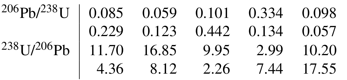
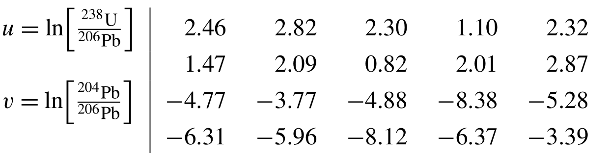
where the subscript c marks the common lead composition, and λ238 is the decay constant of 238U. Equation (1) does not depend on the absolute amounts of 204Pb, 206Pb, and 238U, but only on their ratios. Unfortunately, the statistical analysis of the ratios of strictly positive numbers is full of potential pitfalls, as will be illustrated with an example that was inspired by McLean et al. (2016). Consider a simple dataset of 10 synthetic U–Pb measurements (Table 1).
Table 1A synthetic U–Pb dataset in arbitrary units (e.g. fmol, mV, pA, or kHz).

Let us calculate the 206Pb 238U ratios for these data,
which are needed to solve Eq. (1). Comparing these
ratios with their reciprocals yields two new sets of 10 numbers.
The elementary rules of mathematics dictate that for any two real numbers x and y. In other words, the reciprocal of the reciprocal ratio ought to equal that ratio. Indeed, for our example it is easy to see that and so forth. However, when we take the arithmetic means of the (reciprocal) ratios
and
then we find that
So the reciprocal of the mean reciprocal ratio does not equal the mean of that ratio! This is a counter-intuitive and clearly wrong result. Unfortunately, current algorithms for SIMS data reduction average ratios using the arithmetic mean or perform (linear) regression through ratio data, which causes similar problems (Ogliore et al., 2011). Inaccurate 206Pb 238U ratios inevitably result in inaccurate U–Pb dates, with the degree of inaccuracy scaling with the relative standard deviation of the measured data. Therefore, the numerical example shown in this section is deeply troubling for isotope geochemistry in general and SIMS U–Pb geochronology in particular.
Traditionally, the precision of isotopic data used in U–Pb
geochronology has been calculated as symmetric confidence
intervals. Unfortunately, this is fraught with similar problems as
those discussed in Sect. 2. For example, take the
arithmetic mean () and standard deviation (sx) of the
206Pb 204Pb ratios in Table 1 and construct a Studentised 95 % confidence interval
for .
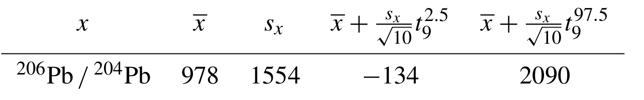
Here, is the α percentile of a t distribution with df degrees of freedom (e.g.
). Then the lower limit of the confidence interval
is negative. This nonsensical result is yet another indication that
there are some fundamental problems with the application of
“conventional” statistical operations to isotopic data. Negative
isotope ratios can also arise from background corrections, but this
will be further discussed in Section 6.
The statistical uncertainty of analytical data can be classified into two components (Renne et al., 1998).
-
Random (or internal) errors are caused by electronic noise in the ion detectors, counting statistics, and/or temporal variability of the background as a result of changes in the lab environment, for example. They are independent for different aliquots of the same sample and can be quantified by taking replicate measurements. The standard error of these measurements (, where σ is the standard deviation of N replicate measurements) is a measure of their precision. The standard error can be reduced to arbitrarily low levels by simply averaging more measurements (i.e. by increasing N). For example, the precision of SIMS 206Pb 204Pb ratio measurements can be increased by simply extending the duration of the primary ion bombardment.
-
Systematic (or external) errors include the effects of decay constant uncertainty and the 206Pb 238U ratio of reference materials. Getting these constants wrong causes bias in some or all of the measurements and thus affects the accuracy of the age determinations. As their name suggests, the systematic uncertainties are not independent but correlated between different aliquots and samples. They cannot be reduced by simple averaging.
Great care must be taken in choosing which sources of uncertainty should or should not be included in the error propagation. In some cases, inter-sample comparisons of SIMS U–Pb data may legitimately ignore systematic uncertainties. However, when comparing data acquired by different methods, both random and some systematic uncertainties must be accounted for. For example, when comparing U–Pb and 40Ar 39Ar data, the decay constant uncertainty must be propagated, and when comparing SIMS and TIMS U–Pb data, SIMS primary standard age uncertainty and the TIMS tracer uncertainty must be propagated. The conventional way to tackle inter-sample comparisons is called “hierarchical” error propagation (Renne et al., 1998; Min et al., 2000; Horstwood et al., 2016). Under this paradigm, the random uncertainties are processed first and the systematic uncertainties afterwards.
Hierarchical error propagation is straightforward in principle but not always in practice. Some processing steps are of a hybrid nature, including both systematic and random uncertainties. 206Pb 238U calibration for SIMS is a good example of this. 206Pb 238U ratios are sensitive to elemental fractionation in SIMS analysis (see Sect. 10 for further details). These fractionation effects are captured by the following power law (Williams, 1998; Jeon and Whitehouse, 2015):
where the subscript m stands for the measured signal ratio, which is generally different from the atomic ratio, and the subscript (2) refers to the fact that the calibration normally uses uranium oxide for SHRIMP and uranium dioxide for Cameca instruments. The atomic 206Pb 238U log ratio of a sample is determined by (1) determining the intercept (A) and slope (B) of a reference material (r) of known Pb U ratio1 and (2) using this calibration curve to estimate the equivalent Pb U log ratio of the reference material corresponding to the UO(2) U log ratio of the sample (s). Then,
where the subscript “a” stands for the estimated (for the sample) or known (for the reference material) atomic log ratios. The analytical uncertainty of depends on the analytical uncertainties of both the intercept (A) and slope (B) of the reference material. But it does not necessarily do so to the same degree for all aliquots. Analytical spots that have similar UO(2) U ratios as the reference material will be less affected by the uncertainty of the reference material fit than spots that have very different UO(2) U ratios (Fig. 1). Hence, it is not possible to make a clean separation between random and systematic uncertainties.
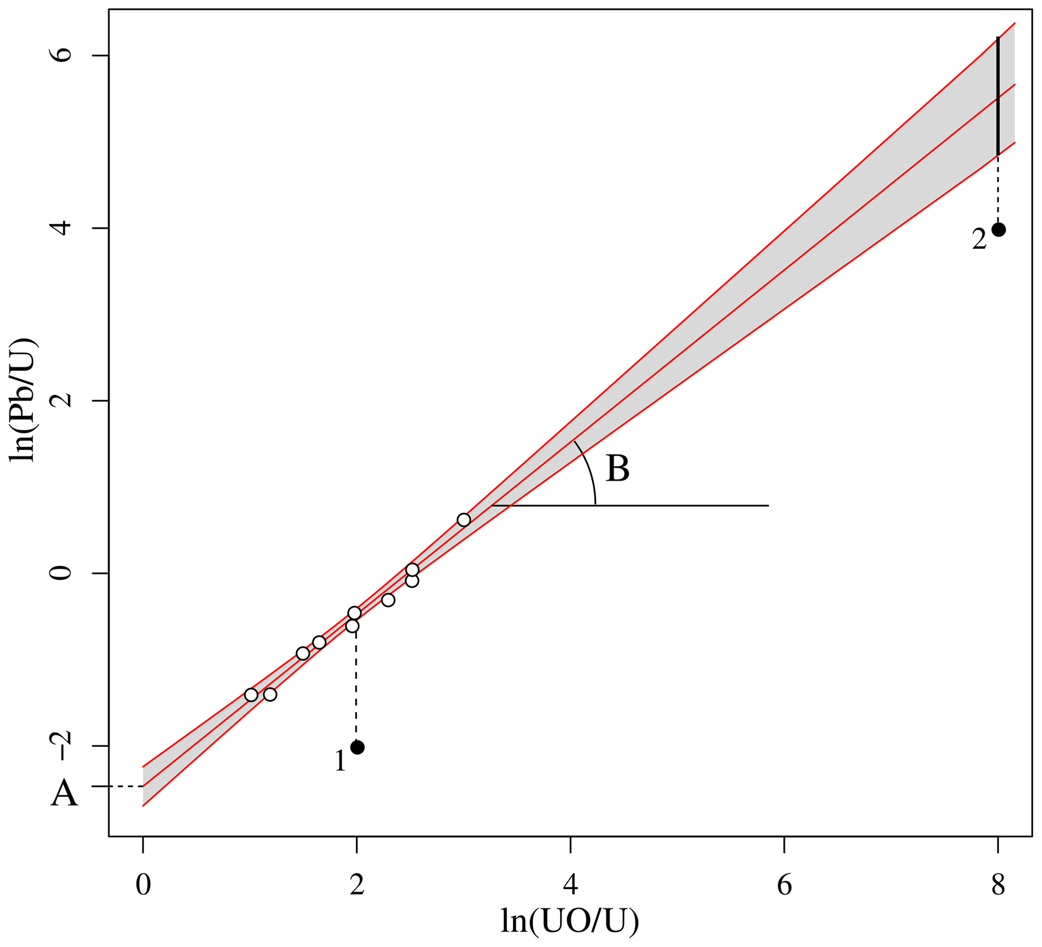
Figure 1SIMS U–Pb calibration curve. White circles mark the isotopic measurements of the reference material and black circles those of two aliquots of the same sample. The uncertainty of the linear fit is shown as a 95 % confidence interval (grey area). This uncertainty can be propagated into the Pb U composition of the sample. It is a systematic uncertainty in the sense that it affects both aliquots. But it does not do so to the same degree. The calibration uncertainty of aliquot 2 is greater than that of aliquot 1 due to its horizontal offset relative to the calibration data.
Section 2 pointed out that the U–Pb age equation (Eq. 1) does not depend on the absolute amounts of 204Pb, 206Pb, and 238U, but only on their relative abundances. Thus, we could normalise the 204Pb, 206Pb, and 238U measurements of Table 1 to unity and plot them on a ternary diagram. The same is true for other geochronometers such as U–Th–He and 40Ar 39Ar (Vermeesch, 2010, 2015). In mathematics, the ternary sample space is known as a two-dimensional simplex. Data that live within this type of space are called compositional data.
Ternary systems are common in igneous petrology (e.g. the A–F–M diagram) and sedimentary petrography (e.g. the Q–F–L diagram). Geologists have long been aware of the problems associated with averages, confidence regions, and linear regression in these closed data spaces (Chayes, 1949, 1960). But a general solution to this conundrum was not found until the 1980s, when the Scottish statistician John Aitchison published a landmark paper and book on the subject (Aitchison, 1982, 1986).
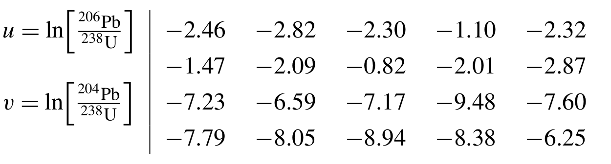
In this work, Aitchison proved that all the problems associated with the statistical analysis of compositional data can be solved by mapping those data from the simplex to a Euclidean space by means of an additive log-ratio (ALR) transformation. For example, given the ternary system , we can define two new variables {u,v} so that
and
In this space, Aitchison showed, one can safely calculate averages and confidence limits. Once the statistical analysis of the transformed data has been completed, the results can then be mapped back to the simplex by means of an inverse log-ratio transformation:
and
For example, the 204,6Pb–238U
system of Table 1 can be mapped from the ternary diagram
to a bivariate
– space.
Alternatively, we could also use 206Pb as the
denominator isotope.
Calculating the average of the transformed data and mapping the
results back to the simplex using the inverse log-ratio transformation
yields the geometric mean of the ratios:
which is an altogether more satisfying result than in
Sect. 2. Moving on to the 95 % confidence intervals
of the 206Pb 204Pb ratios, we
first determine the conventional confidence limits for the log ratios.
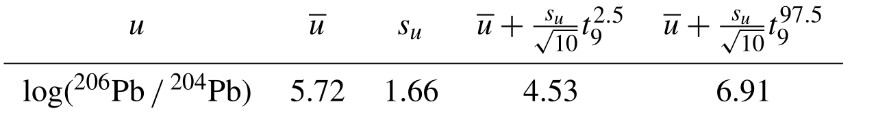
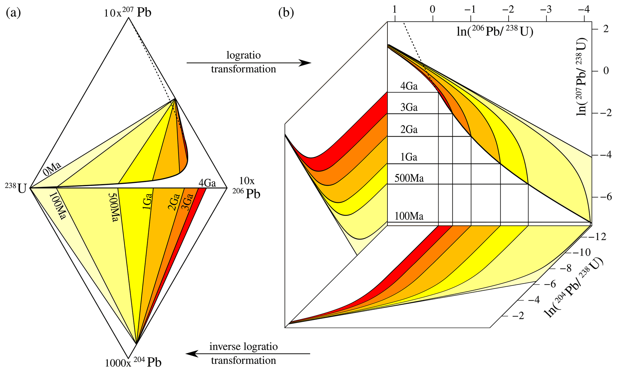
Figure 2The U–Pb age equation (a) projected onto the four-component simplex and (b) mapped to a three-dimensional Euclidean log-ratio space. 235U is omitted from the diagrams because it exists in a constant ratio to 238U (238U 235U = 137.818, Hiess et al., 2012). The boundaries between the coloured regions mark mixing lines between radiogenic and inherited end-member compositions, assuming common Pb ratios of [207Pb 204Pb]c = 10 and [206Pb 204Pb]c = 9. The mixing lines define isochron surfaces that are linear in the simplex and curved in log-ratio space. Rotating the log-ratio plot 90∘ clockwise produces a logarithmic version of the familiar Wetherill concordia diagram. Concordant 206Pb 238U and 207Pb 235U compositions are marked by a thick black line from 0 to 4 Ga and by a dotted line beyond 4 Ga. This paper makes the case that U–Pb data processing is best done in log-ratio space because this “liberates” the data from the geometric constraints of the simplex, producing symmetric uncertainty distributions and more accurate results.
After the inverse log-ratio transformation, these values produce an asymmetric 95 % confidence interval for the geometric mean 206Pb 204Pb ratio of . This interval contains only strictly positive values, solving the problem of Sect. 3. The ALR transformation of Eq. (4) can easily be generalised to more than three components. For example, if 207Pb is added to the mix, then the four-component Pb–238U system can be mapped to the three-component space (Fig. 2).
The compositional nature of isotopic data embeds a covariant structure into the very DNA of geochronology: in a K-component system, increasing the absolute amount of one of the components automatically lowers the relative amount of the remaining (K−1) components (Chayes, 1960). To deal with this phenomenon, it is customary in compositional data analysis to process data in matrix form using the full covariance matrix. For example, four components yield three log ratios, which require a 3×3 covariance matrix to describe the uncertainties and uncertainty correlations.
This approach is now widely used in sedimentary geology, geochemistry, and ecology (e.g. Weltje, 2002; Vermeesch, 2006; Pawlowsky-Glahn and Buccianti, 2011), and it has recently been adopted for geochronological applications as well (Vermeesch, 2010, 2015; McLean et al., 2016). The log-ratio covariance matrix approach is also uniquely suited to capture the systematic uncertainties (i.e. the inter-spot error correlations) that are produced by the SIMS U–Pb calibration procedure (Sect. 4). In that case, the covariance matrix must be expanded to accommodate multiple spots (e.g. Vermeesch, 2015). For example, the covariance structure of three spots in a four-component system can be captured in a 9×9 matrix.
In conclusion, the log-ratio transformation solves the statistical woes described in Sects. 2, 3, and 4 of this paper. However, there are two additional problems that require further remediation.
Many mathematical operations are easier in logarithmic space than in linear space: multiplication becomes addition, division becomes subtraction, and exponentiation becomes multiplication. These mathematical operations are very common in mass spectrometer data processing chains (Vermeesch, 2015). However, there are exceptions. For example, background correction does not involve the multiplication but subtraction of two signals. For low-intensity ion beams such as 204Pb, it is possible, by chance, that the background exceeds the signal. This results in negative values of which one cannot take the logarithm.
The subtraction problem can be solved by using a different logarithmic change of variables:
where x and y are the signals and b is the background. The infinite space of covers all possible values of x, y, and b for which x>b and y>b. Thus, background correction should be done in β space, given an appropriate error model as described in Sect. 7.
One caveat to this background correction method is that it does not account for isobaric interferences, which may result in “overcounted” signals. The high mass resolution of SIMS instruments removes most but not all isobaric interferences. For example, spurious HfSi, REE dioxide, or long-chain hydrocarbon ions can interfere with 204Pb, which is generally the rarest isotopic species detected. If unaccounted for, these interferences lead to the proportion of non-radiogenic Pb being overestimated (and the proportion of radiogenic Pb underestimated), resulting in excessive common Pb corrections and underestimated dates. The accuracy of the background measurements can be monitored via the use of isotopically homogeneous reference materials (Black, 2005). A correction can then be applied by choosing the “session blank” that brings the common Pb-corrected 207Pb 206Pb ratios in alignment with the reference values.
Another issue arises when SIMS signals are registered by secondary electron multiplier (SEM) detectors. These record ion beams as discrete counts, i.e. as integers, which are incompatible with the log-ratio transformation. For example, it is not uncommon for SEM detectors to register zero counts for low-intensity ion beams such as 204Pb. These zero counts blow up the log-ratio transformation because .
This and other issues are diagnostic of a fundamental difference between compositional data and counting data that has been previously recognised and solved in fission-track dating (Galbraith, 2005) and in sedimentary petrography (Vermeesch, 2018b). The same solutions can be applied to mass spectrometric count data in general and to U–Pb geochronology in particular (Sect. 7).
Standard data reduction procedures for geochronology assume normally distributed residuals. In compositional data analysis, these are replaced by logistic normal distributions. However, neither the normal nor the logistic normal distribution is perfectly suited to dealing with discrete count data. The multinomial distribution is a simple alternative that seems more appropriate for the task at hand. Before we proceed, let us define the following variables.
-
ϕx and ϕb are the normalised true ion beam intensities (in counts per second) of mass x (from a set of monitored masses 𝕩) and the normalised background signal, respectively, so that
-
dx and db are the dwell times of mass x and the background b
-
θx and θb are the normalised expected beam counts of the ions and the background so that
and
Using the 204Pb 206Pb ratio as an example, the probability of observing n4 counts at mass 204, n6 counts at mass 206, and nb counts of background is given by
Whereas the observations n4, n6, and nb are integers, the parameters θ4, θ6, and θb are decimal numbers that are constrained to a constant sum. In other words, they belong to the simplex. Thus, we can map the three multinomial parameters to two log-ratio parameters, thereby establishing a natural link between counting data and compositional data. For example,
and
and can be estimated from n4, n6, and nb by maximising the likelihood defined by Eq. (10).
The normal and logistic normal distributions are controlled by two sets of parameters: location parameters and shape parameters. In the case of the normal distribution, the location parameter is the mean and the shape parameter is the standard deviation (or covariance matrix). In contrast, the multinomial distribution has only one set of (θ) parameters. The precision of multinomial counts is governed by the number of observed counts (). More sophisticated models are possible when the observed dispersion of the data exceeds that which is expected from the multinomial counting statistics (e.g. Galbraith and Laslett, 1993; Vermeesch, 2018b). However, in this paper we will assume that such overdispersion is absent from the reference materials and from the single-spot analyses.
It takes a few tens of nanoseconds for a secondary electron multiplier to record the arrival of an ion. During this “dead time”, the detector is unable to register the arrival of additional ions. This phenomenon can significantly bias isotope ratio estimates that include ion beams of contrasting intensity. Fortunately, the dead-time effect can be easily corrected. It suffices that the dwell times are adjusted by the cumulative amount of time that the detectors were incapacitated. Let be the “effective dwell time” of ion beam x:
where δx is the (non-extended) dead time of the detector that measures x. Then the expected normalised beam counts can be re-defined as
and the normalised beam intensities as
The difference between this approach and existing SIMS data reduction approaches is that conventional data reduction algorithms apply the dead-time correction to the raw data before calculating isotopic data, whereas the new method applies the dead-time correction to and , which are unknown parameters that must be estimated from the data.
Thus far we have assumed that all ions are measured synchronously, which is the case in multicollector configurations. However, in single-collector experiments, the measurements are made asynchronously. This can cause biased results if the signals drift over time. In SHRIMP data processing, it is customary to correct this drift by normalising to a secondary beam monitor (SBM) signal2, followed by double interpolation of numerator and denominator isotopes (Bodorkos et al., 2020; Dodson, 1978). A unified data reduction algorithm for SHRIMP and Cameca instruments requires a different approach, in which the time dependency of the signals is parameterised using a log-linear model. For Faraday detectors,
where is the ion beam intensity of the ith integration for mass x of element X evaluated at time , σ is the standard deviation of the normally distributed data scatter around the best fit line, and “bkg” is the background signal. This is usually a nominal value for Cameca instruments and an actual set of measurements () for SHRIMP data. Note that the intercept parameters (αx) are ionic-mass-specific, whereas the slopes (γX) are element-specific. See the Appendix for an example. For SEM detectors, the scatter of the data around the log-linear fit is controlled by Poisson shot noise:
The background-corrected signal ratio (evaluated at ) for two ion beams x and y of different elements X and Y can then be drift-corrected as follows:
where and are the dead-time-corrected normalised beam intensities for the ith integration of masses x and y, respectively, and is the corresponding background value. See the Appendix for further details.
Mass spectrometer signals are recorded in volts (for Faraday detectors) or hertz (or secondary electron multipliers). The age equation, however, requires atomic ratios. In general, signal ratios do not equal atomic ratios because they are affected by two types of fractionation.
-
Mass-dependent fractionation. The Pb isotopes span a range of four mass units, with 208Pb being 2 % heavier than 204Pb. Both the production and detection efficiency of secondary ions vary with atomic mass, and significant errors can potentially occur if the resulting mass fractionation is uncorrected for. Mass fractionation can be quantified by comparing the measured signal ratios of a reference material with its known isotopic ratio. This is easy to do in a log-ratio context (Vermeesch, 2015).
-
Elemental fractionation. The fractionation between the Pb isotopes is caused by (slight) differences in their physical properties, i.e. their mass. As briefly mentioned in Sect. 4, much stronger fractionation effects tend to occur between the isotopes and Pb and U because they are not only physically but also chemically different. These chemical differences affect the complex processes that occur when the primary ion beam interacts with the target material (Williams, 1998).
In the context of SIMS U–Pb geochronology, mass-dependent fractionation is commonly ignored (but not always, e.g. Stern et al., 2009) because the most important isochemical ratio is that between 206Pb and 207Pb, which lie within 0.5 % mass units of each other. This is unresolvable given typical analytical uncertainties. The mass fractionation is greater for 204Pb, but so is its analytical uncertainty. Therefore, the atomic 204Pb 206Pb, 207Pb 206Pb, and 208Pb 206Pb ratios can be directly estimated from the (drift-corrected) 204Pb 206Pb, 207Pb 206Pb, and 208Pb 206Pb signal ratios. This is not the case for the 206Pb 238U and 208Pb 232Th ratios, which are affected by strong elemental fractionation effects. This fractionation expresses itself in two ways.
-
Within-spot fractionation
Over the course of a SIMS spot analysis, the Pb U and Pb Th ratio changes as a function of time. This elemental fractionation can be modelled using a log-linear model that is similar to that used for the within-spot drift correction:
where is the inferred log ratio of the background-corrected signals at “time zero”, which can be found using the method of maximum likelihood (see the Appendix). Note that if X=Y, and, if the sensitivity drift of the data is smooth and closely follows the trends defined by Eqs. (16) and (17), then and .
Using Eq. (19), the isotopic log ratios can be interpolated (or extrapolated) to any point in time (τ):
The most precise values of are obtained when τ is chosen in the middle of the analytical sequence. These values can be used for subsequent calculations. Alternatively, we can also use the time-zero intercepts .
-
Between-spot fractionation
The Pb U and Pb Th signal ratios may vary between adjacent spots on the same isotopically homogenous reference material. This fractionation obeys the power-law relationship given by Eq. (2). Expressing this formula in terms of corrected signal ratios gives
where stands for the 206Pb 204Pb ratio of the common Pb (see the footnote of Sect. 4). Recasting Eq. (21) in terms of the interpolated log-ratio estimates gives
where “o” stands for the uranium oxide (238U16O or 238U16O+) and “u” stands for 238U+.
Having applied Eq. (22) to a reference material with a known atomic 206Pb 238U ratio , the atomic 206Pb 238U ratio of the sample is given by
where and are the interpolated log-ratio estimates of the sample. The 206Pb 238U age is then obtained by plugging into the age equation. Uncertainties are obtained by standard error propagation (see the Appendix).
The following paragraphs will illustrate the SIMS U–Pb data reduction process using two datasets.
-
Dataset 1 was acquired by Yang Li at IGG-CAS Beijing using a Cameca 1280HR instrument with five SEMs and two Faraday detectors run in single-collector mode using an SEM for all mass stations. The dataset uses Temora2 zircon (416.8 ± 1.1 Ma, Black et al., 2004) as a reference material and 91500 zircon (1062.4 ± 0.2 Ma, Wiedenbeck et al., 1995) as a sample. Measurements consist of seven cycles through a set of 11 mass stations per single-spot measurement for 90Zr2O (0.48 s dwell time per cycle), 92Zr2O (0.08 s), mass 200.5 (background, 4.00 s), 94Zr2O (0.32 s), 204Pb (4.96 s), 206Pb (2.96 s), 207Pb (6.00 s), 208Pb (2.00 s), 238U (2.96 s), ThO2 (2.96 s), and UO2 (2.96 s).
-
Dataset 2 was acquired by Simon Bodorkos at Geoscience Australia using a single-collector SHRIMP-II instrument, employing an SEM for all mass stations. This dataset also uses Temora2 as a reference material, as well as 91500 zircon, OG.1 (3440.7 ± 3.2 Ma, Stern et al., 2009), and M127 (524.36 ± 0.16 Ma, Nasdala et al., 2016) as samples. Measurements consist of six cycles through a set of 10 mass stations per single-spot measurement for 90Zr2O (2.0 s dwell time per cycle), 204Pb (20 s), mass 204.04091 (background, 20 s), 206Pb (15 s), 207Pb (40 s), 208Pb (5 s), 238U (5 s), ThO (2 s), UO (2 s), and UO2 (2 s).
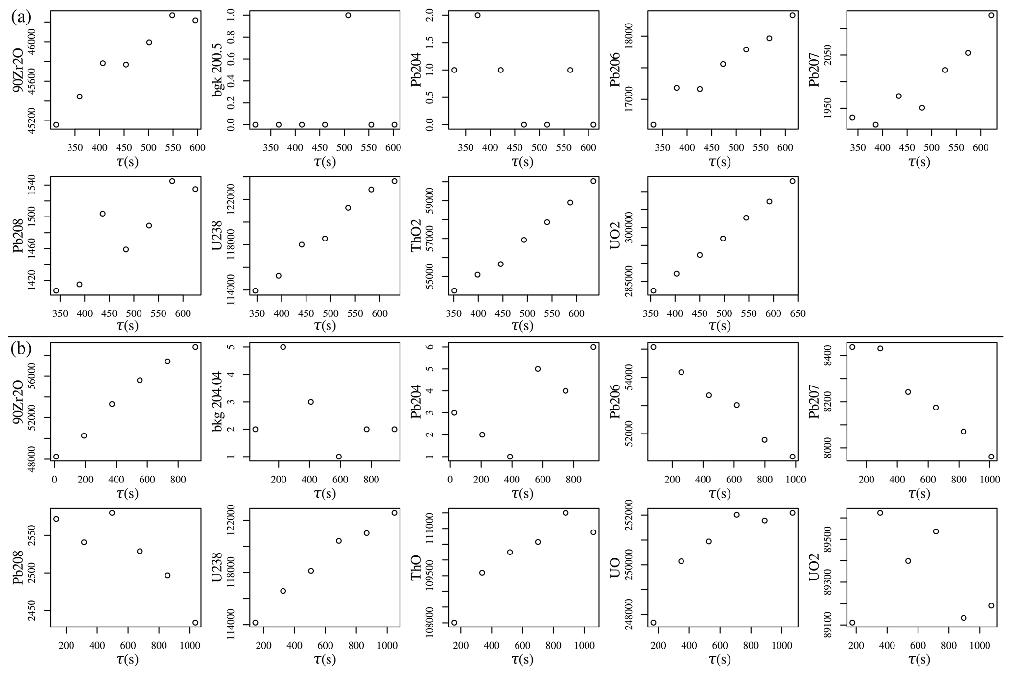
Figure 3Time-resolved signals (counts) of (a) Temora2 (spot
Tem@6) analysed by a Cameca 1280HR instrument at IGG-CAS
Beijing; (b) M127 zircon (spot M127.1.2) analysed by a
SHRIMP-II instrument at Geoscience Australia.
Figure 3 shows the time-resolved SEM counts of one representative spot measurement for each dataset. Side-by-side comparison of these two datasets reveals some interesting similarities and differences. All of the high-intensity signals exhibit clear transient behaviour, which is caused by changes in oxygen availability that occur during primary ion bombardment (Magee et al., 2017). The transience of the individual SEM signals biases the isotopic ratios. For example, there are 109 s between the 204Pb and 208Pb measurements in each SHRIMP cycle. During these 109 s, the 208Pb signal drops on average by 2 %, resulting in an equivalent bias of the 204Pb 208Pb ratio (Sect. 9). A similar drop per cycle is observed for the Cameca data.
However, there is a key difference between the Cameca and SHRIMP datasets. For the Cameca data, the U and Pb signals both drift in the same direction, resulting in positive slopes for the example of Fig. 3. But for the SHRIMP data, the U and Pb drift in opposite directions: the U signal exhibits an increase in sensitivity with time, whereas the Pb signals decrease in intensity with time. This marked difference in behaviour between the two instruments reflects a difference in their design, causing a difference in the energy window of the secondary ions analysed (Ireland and Williams, 2003).
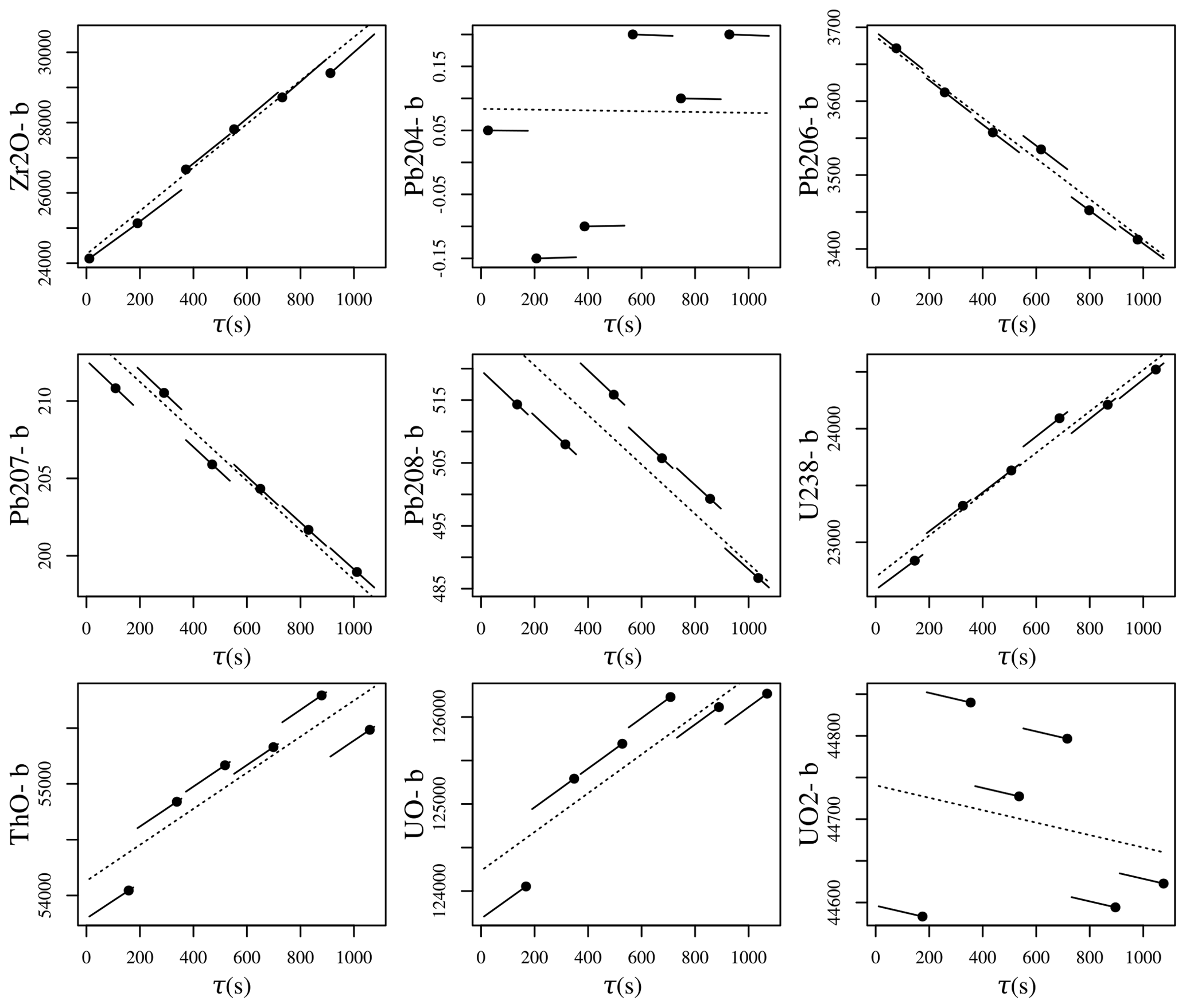
Figure 4Within-spot drift correction of the background-corrected SHRIMP data from Fig. 3. Dotted lines are log-linear functions whose element-specific slopes (γX in Eq. 17) are used for the drift correction but for no other purpose. Solid lines mark the duration of each mass spectrometer cycle, with the black dots representing the starting point of each individual mass station within the cycles. The solid lines are parallel to the dotted lines (in log space) and express how the isotope ratio fits can be translated to match the asynchronous mass spectrometer signals. Vertical axes have units of counts per second.
For Faraday detectors, the within-spot drift correction uses a generalised linear model with a lognormal link function (Eq. 16). For SEM data, it uses a Poisson link function (Eq. 17). In either case, the model enforces strictly positive isotopic abundances. Isotopes of the same element (such as Pb) have the same slope parameter but different intercepts. Isotopes of different elements are free to have different slopes (Fig. 4).
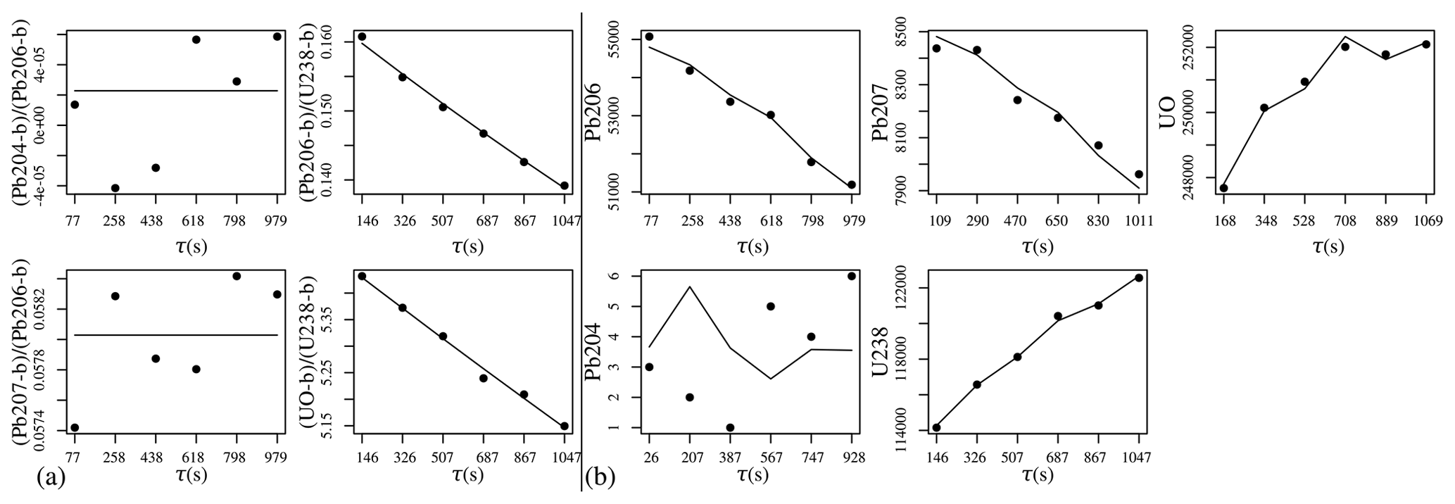
Figure 5(a) Background- and drift-corrected ratio fits to the SHRIMP data from Fig. 3, obtained using the generalised linear model of Eq. (19). The slope parameter ( in Eq. 19) is zero for isotopes of the same element and non-zero for isotopes of different elements. Vertical axes are unitless. (b) The four (log-)ratio fits can be converted back to five isotope signal fits using the inverse log-ratio transformation. Multiplying the normalised ion beam intensity fits with the total number of counts per sweep allows direct comparison with the raw measurements, which are shown as filled circles. Vertical axes have units of counts. Note that the measurements have Poisson uncertainties, which scale with the square root of the values.
Figure 5 applies another log-linear function (Eq. 19) to model the within-spot fractionation of SHRIMP Temora2 spot 11. This function models the drift-corrected log ratios as a linear function of analysis time. The slopes of the log-linear functions are a function of the within-spot fractionation between the numerator and denominator elements. Because there is no fractionation between two isotopes of the same element, the slope of the Pb Pb ratios is zero.
The ability of log-ratio statistics to avoid negative ratios is apparent from the first panel of Fig. 5. Even though some of the the background-corrected ratio signals are zero or negative (because the background exceeded the signal), the generalised linear fit is strictly positive. The natural ability of compositional data analysis to rule out negative ratios avoids many problems further down the data processing chain.
The right-hand side of Fig. 5 maps the four (log) ratios back to five equivalent raw signals (one for each isotope). The last two panels of the figure show how the log-ratio approach manages to effectively capture subtle fluctuations of the U and UO signal intensities.

Figure 6(a) U–Pb calibration curve for the Temora2 SHRIMP data using the time-zero (τ=0) intercepts (green ellipses). Black and white dots mark the first and last cycles of each analysis, respectively. (b) The log-ratio data and calibration fit for the same data, but evaluated at the midpoint (τ=544), resulting in a more precise calibration. All uncertainties are shown at 95 % confidence.
The log-ratio intercepts obtained by Eq. (19) form a linear array of calibration data (Eq. 22). Figure 6a fits a straight line through these points using the linear regression algorithm of York et al. (2004). Alternatively, instead of fitting a calibration line through the log-ratio intercepts (τ=0, Fig. 6a), it is also possible to interpolate or extrapolate the log-ratio composition to any other point in time. For example, the green ellipses in Fig. 6b show the inferred log-ratio compositions at 544 s (i.e. τ=544), which represents the midpoint of the analyses. The slope of this calibration line is notably different than that obtained by fitting a line through the compositions at 0 s. This change in slope reflects the different mechanisms that are responsible for elemental fractionation within and between SIMS spots.
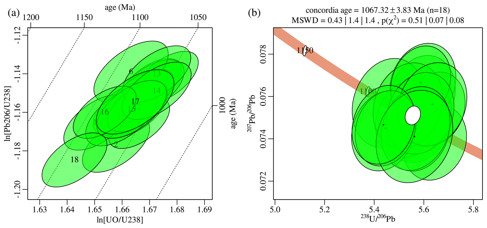
Figure 7(a) Calibration plot of the SHRIMP 91500 zircon data using
Temora2 as a reference material. Dotted lines are parallel to the
regression line of Fig. 6b. (b) The same data
shown on a Tera–Wasserburg concordia diagram, which was obtained
with IsoplotR and does not take into account systematic
errors associated with the calibration fit. All uncertainties are shown at 95 % confidence. The white ellipse marks the weighted mean composition, with MSWD and p values
representing the goodness of fit for equivalence, concordance, and
equivalence+concordance.
Table 2Uncertainty budget of the four Temora2 zircon analyses highlighted in Fig. 8. The first two data columns show the calibrated 206Pb 238U log ratios and their standard errors ignoring the uncertainty of the calibration fit (i.e. using internal uncertainties only). The third column shows the total error including the external uncertainty associated with the calibration fit. The upper triangular matrix shown in the remaining three columns contains the (total) error correlations of the four aliquots.
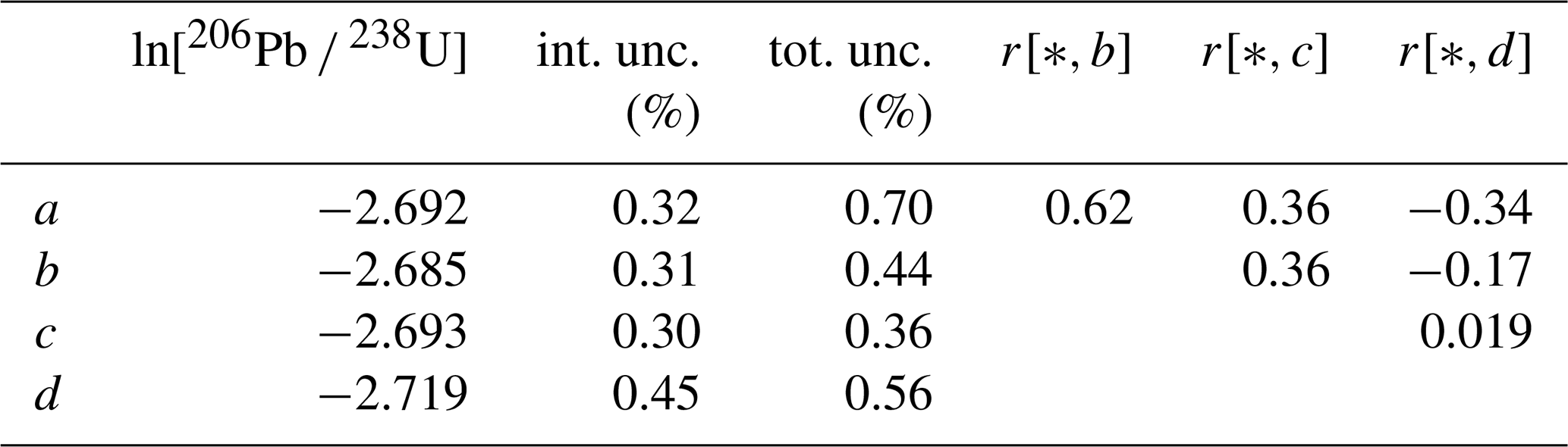
Figure 7 applies the Pb U calibration (Eq. 23) to 91500 zircon using the Temora2 data for calibration. It shows only the purely random errors, i.e. ignoring the uncertainty of the calibration. Including the calibration errors not only inflates the uncertainties, but also causes inter-spot error correlations (Fig. 1). To demonstrate this phenomenon, let us revisit the Cameca data and swap the sample and reference materials around. Thus, we use 91500 for the calibration curve and Temora2 as a sample (Fig. 8). Table 2 shows the uncertainty budget of four selected aliquots from this sample.
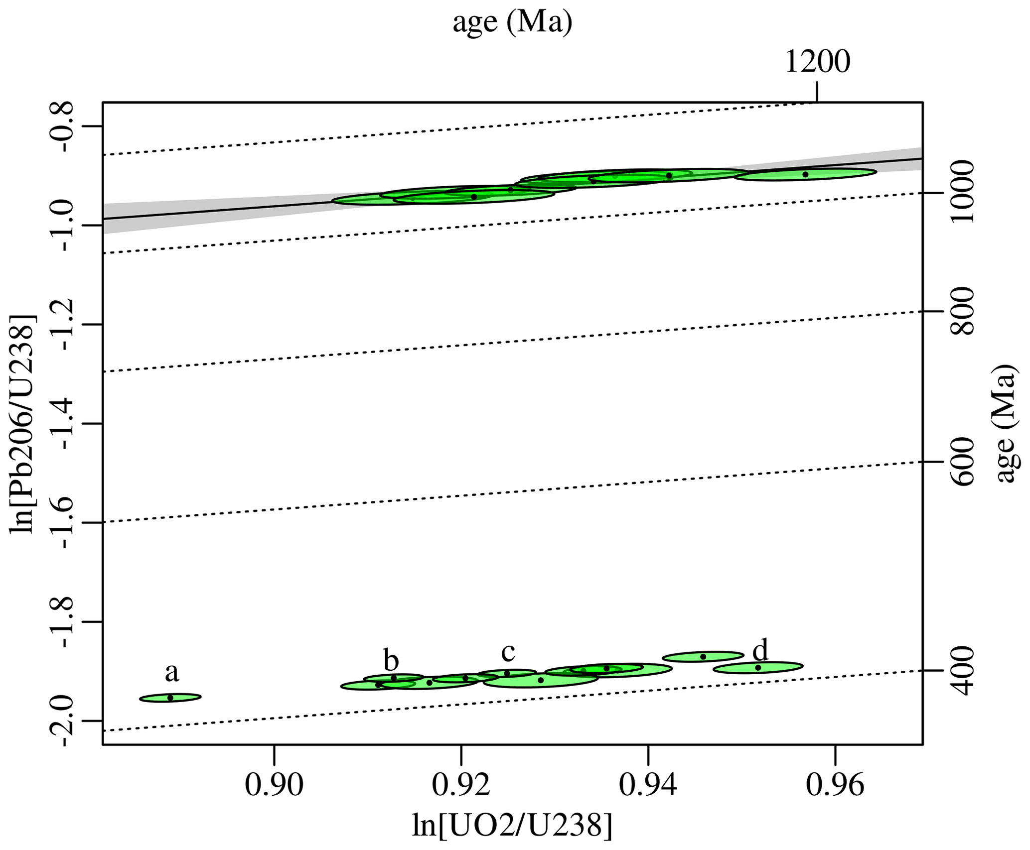
Figure 8Calibration curve of the Cameca data using 91500 zircon as a reference material (top half of the plot) and Temora2 zircon as a sample (bottom half). a–d mark four Temora2 aliquots whose uncertainty budget is explored in Table 2.
Propagating the calibration curve uncertainty increases the error estimates (Table 2) by different amounts for different spots. For aliquot c, which is located immediately below the mean of the 91500 data, the calibration uncertainty only mildly increases the standard error from 0.30 % to 0.36 %. However, for aliquot a, which is horizontally offset from the mean of the calibration data, the systematic calibration uncertainty more than doubles the standard error from 0.32 % to 0.70 %. The calibration error also causes the standard errors of the various aliquots to be correlated with each other. For example, the total uncertainties of aliquots a and b are positively correlated () because their UO2 U ratios are both offset from the mean of the calibration in the same direction. In contrast, the uncertainties of aliquots a and d are negatively correlated () because they are offset in opposite directions from the mean of the calibration data.
The inter-spot error correlations are important when calculating
weighted means (Vermeesch, 2015) and isochrons. Taking into
account the full covariance structure of the data affects both the
accuracy and the precision of any derived age information. For
example, the conventional weighted mean can be replaced with a matrix
expression that accounts for correlated uncertainties
(Eq. 92 of Vermeesch, 2015). Applying this modified
algorithm to the positively correlated aliquots a and b of
Table 2 changes the weighted mean from −2.6922
to −2.6854 and increases the standard error of that mean from 0.37 %
to 0.44 %. Applying the same calculation to the negatively correlated
aliquots a and d changes their weighted mean from −2.7083 to
−2.7076 and reduces uncertainty from 0.43 % to 0.35 %. To take
full advantage of the covariance matrix will require the development
of a new generation of high-level data reduction software. For
example, future versions of IsoplotR (Vermeesch, 2018a)
will be modified to handle these rich data structures. A
comprehensive discussion of this topic falls outside the scope of this
paper.
R package simplex The SIMS data processing algorithm presented in this paper is implemented in an R package called simplex. The programme
can be run in three modes: online, offline, and from the command
line. The online version can be accessed at
https://isoplotr.es.ucl.ac.uk/simplex/ (last access: 16 August 2022). It contains three example U–Pb datasets, including the two datasets used in this paper, plus a Cameca monazite U–Th–Pb dataset.
The simplex package currently accepts raw data as Cameca .asc
and SHRIMP .op and .pd files. Support for SHRIMP
.xml files will be added later. The online version is a good
place to try the look and feel of the software. However, it is
probably not the most practical way to process lots of large data
files. For a more responsive user experience, simplex can
also be run natively on any operating system (Windows, Mac OS, or
Linux). To this end, the user needs to install R on their
system (see https://r-project.org/ for details, last access: 16 August 2022). Within
R, the simplex package can be installed from the
GitHub code-sharing platform using the remotes
package by entering the following commands at the console.
install.packages("remotes")
remotes::install_github("pvermees/simplex")
Once installed, the simplex graphical user interface (GUI) can
be started by entering the following command at the console.
simplex::simplex()
A third and final way to use simplex is from the command
line. This allows advanced users to create automation scripts and
extend the functionality of the package. The simplex package comes with
an extensive API (Application Programming Interface) of fully
documented user functions. An overview of all these functions can be
obtained by typing the following command at the console.
help(package="simplex")
This paper introduced a new algorithm for SIMS U–Pb geochronology, in which raw mass spectrometer signals are processed using a combination of log-ratio analysis and Poisson counting statistics. In contrast with existing data reduction protocols, which handle each aliquot of an analytical sequence separately, the new algorithm simultaneously processes all of them in parallel. It thereby produces an internally consistent set of isotopic ratios and their associated covariance matrix. This covariance matrix is a rich source of information that captures both random and systematic uncertainties, including inter-spot error correlations that have hitherto been ignored in geochronology.
The example data of Sect. 12 showed that these
inter-spot error correlations can be either positive or negative
(see also Vermeesch, 2015; McLean et al., 2016). Ignoring them affects
both the accuracy and precision of high-end data processing steps such
as isochron regression and concordia age calculation. Unfortunately,
existing postprocessing software such as Isoplot
(Ludwig, 2003) and IsoplotR (Vermeesch, 2018a) does
not yet handle inter-spot error correlations. Further work is needed
to extend these codes and take full advantage of the new
algorithm. IsoplotR was designed with such future upgrades in
mind: its input window contains a large number of spare columns that
will accommodate covariance matrices in a future update. Once the
aforementioned high-end data reduction calculations have been updated,
it will be possible to fully quantify the gain in precision and
accuracy of the new algorithm compared to the previous generation of
SIMS data reduction software.
The data reduction principles laid out in this paper are applicable
not only to U–Pb geochronology, but also to other SIMS applications
such as stable isotope analysis. In fact, simplex already
handles such data for multicollector Cameca instruments. It is worth
mentioning that the stable isotope functionality can also be used to
correct 207Pb 206Pb ratio
measurements for mass-dependent isotope fractionation, as was briefly
discussed in Sect. 10. Future updates of the
mass-dependent fractionation correction will also address the
overcounted background problem that was mentioned in
Sect. 6.
Besides U–Pb geochronology and stable isotopes, the new data
reduction paradigm can also be adapted to other chronometers and other
mass spectrometer designs, such as thermal ionisation mass
spectrometry (TIMS, Connelly et al., 2021), noble gas mass
spectrometry (Vermeesch, 2015), and LAICPMS (McLean et al., 2016).
The simplex package already includes a function to export data to
IsoplotR. Adding similar functionality to other data
processing software will improve geochronologists' ability to
integrate multiple datasets whilst keeping track of systematic
uncertainties, including those associated with reference materials and
decay constants.
This section provides further algorithmic details for the new U–Pb data processing workflow. It assumes that ions are recorded on SEM detectors, which is by far the most common configuration. The case of Faraday collectors is similar and, in fact, simpler.
Within-spot drift is modelled using a log-linear function (Eq. 17) with a distinct intercept (αx) for each ion channel (x) and shared slopes (γX) between isotopes of the same element (X). To illustrate this concept, consider the case of Pb (inclusion of 208Pb is a trivial extension). Let be the time-dependent parameter of the shot noise for 20xPb, where :
Then the log-likelihood function of the parameters given the data is defined as
where N represents the number of cycles. The parameters and γPb are estimated by maximising ℒℒd with respect to them. Only γPb is used in subsequent calculations. The intercepts α{x} are discarded.
The next step of the data reduction extracts log ratios from the raw data using a log-linear model that is similar to the within-spot drift correction (Eq. 19). Here, in contrast with the drift correction, the intercepts are just as important as the slopes. For isochemical ratios such as 207Pb 206Pb, the slope of the drift-corrected log ratios is zero and we only need to estimate the intercept. For multichemical ratios such as 238U 206Pb, both the slope and the intercept are non-zero. In order to keep track of covariances, it is useful to process all the isotopes together using a common denominator. For example, using 206Pb (6) as a common denominator and 204Pb (4), 207Pb (7), 238U (u), and UO (o) as numerators,
where X stands for Pb if , for U if x=u, and for UO if x=o. Then the normalised ion counts are given by
and
for , with
in which . Then the log-likelihood is calculated as
where because there is no elemental fractionation between the Pb isotopes. From the log ratios with a common denominator, it is easy to derive any other log ratio:
One of the main advantages of the new data reduction method is its ability to keep track of the full covariance structure of the data, including inter-spot error correlations. This ability is derived from the fact that all parameters are derived by the method of maximum likelihood, which stipulates that the approximate covariance matrix of any set of estimated parameters can be obtained by inverting the negative matrix of second derivatives (i.e. the Hessian matrix) of the log-likelihood function with respect to said parameters.
For example, to estimate the covariance matrix of the log-ratio slopes and intercepts for a single-spot analysis, the Hessian is a 6×6 matrix that includes the second derivatives of ℒℒl with respect to , , , , , and . Computing this matrix is tedious to do by hand but straightforward to do numerically.
Given the covariance matrix of the log ratios, subsequent data reduction steps propagate the analytical uncertainties by a conventional first-order Taylor approximation. Thus, if y=f(x), then
where Jf is the Jacobian matrix (and its transpose) of partial derivatives of f with respect to x. For example, to estimate the m×m covariance matrix of m fractionation-corrected 206Pb 238U ratios, error propagation of Eq. (23) would involve an Jacobian matrix and a covariance matrix containing the uncertainties of A, B, and , as well as and (for j from 1 to m).
The source code, installation instructions, and example datasets for simplex can be accessed at https://github.com/pvermees/simplex/ (last access: 16 August 2022; https://doi.org/10.5281/zenodo.6954203, Vermeesch, 2022).
The author is a member of the editorial board of Geochronology.
Publisher's note: Copernicus Publications remains neutral with regard to jurisdictional claims in published maps and institutional affiliations.
The idea for this work was born during an academic visit of the author
to the Institute of Geology and Geophysics (IGG) at the Chinese
Academy of Sciences (CAS) in Beijing. With no prior experience in
handling SIMS data, the author relied on the expertise of Yang Li
and Li-Guang Wu (IGG-CAS) to introduce him to the world of Cameca data processing, as well as of Simon Bodorkos, Charles Magee, and Andrew Cross (Geoscience Australia) for SHRIMP data processing. The test data were kindly shared by Yang Li and Simon Bodorkos, who also provided detailed feedback on the paper prior to submission. Software development for the simplex
data reduction programme was supported by NERC standard grant
NE/T001518/1 (“Beyond Isoplot”), which aims to develop an
“ecosystem” of interconnected geochronological data processing
software. The graphical user interface for simplex makes
extensive use of the shinylight and dataentrygrid
packages developed by software engineer Tim Band, who is employed on
this NERC grant.
This research has been supported by the Natural Environment Research Council (grant no. NE/T001518/1).
This paper was edited by Noah M. McLean and reviewed by Morgan Williams and Nicole Rayner.
Aitchison, J.: The Statistical Analysis of Compositional Data, J. Roy. Stat. Soc., 44, 139–177, 1982. a
Aitchison, J.: The statistical analysis of compositional data, London, Chapman and Hall, ISBN 0412280604, 1986. a
Black, L. P.: The use of multiple reference samples for the monitoring of ion microprobe performance during zircon 207Pb 206Pb age determinations, Geostand. Geoanal. Res., 29, 169–182, 2005. a
Black, L. P., Kamo, S. L., Allen, C. M., Davis, D. W., Aleinikoff, J. N., Valley, J. W., Mundil, R., Campbell, I. H., Korsch, R. J., Williams, I. S., and Foudoulis, C.: Improved 206Pb 238U microprobe geochronology by the monitoring of a trace-element-related matrix effect; SHRIMP, ID–TIMS, ELA–ICP–MS and oxygen isotope documentation for a series of zircon standards, Chem. Geol., 205, 115–140, 2004. a
Bodorkos, S., Bowring, J., and Rayner, N.: Squid3: Next-generation Data Processing Software for Sensitive High Resolution Ion Micro Probe (SHRIMP), Geoscience Australia, https://doi.org/10.11636/133870, 2020. a, b
Chayes, F.: On ratio correlation in petrography, J. Geol., 57, 239–254, 1949. a
Chayes, F.: On correlation between variables of constant sum, J. Geophys. Res., 65, 4185–4193, 1960. a, b
Connelly, J., Bollard, J., Costa, M., Vermeesch, P., and Bizzarro, M.: Improved methods for high-precision Pb–Pb dating of extra-terrestrial materials, J. Anal. Atom. Spectrom., 36, 2579–2587, 2021. a
Dodson, M.: A linear method for second-degree interpolation in cyclical data collection, J. Phys. E Sci. Instrum., 11, 296, https://doi.org/10.1088/0022-3735/11/4/004, 1978. a
Galbraith, R. F.: Statistics for fission track analysis, CRC Press, 2005. a
Galbraith, R. F. and Laslett, G. M.: Statistical models for mixed fission track ages, Nucl. Tracks Rad. Meas., 21, 459–470, 1993. a
Hiess, J., Condon, D. J., McLean, N., and Noble, S. R.: 238U 235U systematics in terrestrial uranium-bearing minerals, Science, 335, 1610–1614, 2012. a
Horstwood, M. S., Košler, J., Gehrels, G., Jackson, S. E., McLean, N. M., Paton, C., Pearson, N. J., Sircombe, K., Sylvester, P., Vermeesch, P., and Bowring, J. F.: Community-Derived Standards for LA-ICP-MS U-(Th-) Pb Geochronology–Uncertainty Propagation, Age Interpretation and Data Reporting, Geostand. Geoanal. Res., 40, 311–332, 2016. a
Ireland, T. R. and Williams, I. S.: Considerations in zircon geochronology by SIMS, Rev. Mineral. Geochem., 53, 215–241, 2003. a
Jeon, H. and Whitehouse, M. J.: A critical evaluation of U–Pb calibration schemes used in SIMS zircon geochronology, Geostand. Geoanal. Res., 39, 443–452, 2015. a
Ludwig, K. R.: Decay constant errors in U–Pb concordia-intercept ages, Chem. Geol., 166, 315–318, 2000. a
Ludwig, K. R.: User's manual for Isoplot 3.00: a geochronological toolkit for Microsoft Excel, Berkeley Geochronology Center Special Publication, vol. 4, 2003. a
Magee, C., Danisik, M., and Mernagh, T.: Extreme isotopologue disequilibrium in molecular SIMS species during SHRIMP geochronology, Geoscientific Instrumentation, Methods and Data Systems, 6, 523–536, 2017. a
McLean, N. M., Bowring, J. F., and Gehrels, G.: Algorithms and software for U-Pb geochronology by LA-ICPMS, Geochem. Geophy. Geosy., 17, 2480–2496, 2016. a, b, c, d
Min, K., Mundil, R., Renne, P. R., and Ludwig, K. R.: A test for systematic errors in 40Ar 39Ar geochronology through comparison with U Pb analysis of a 1.1-Ga rhyolite, Geochim. Cosmochim. Ac., 64, 73–98, 2000. a
Nasdala, L., Corfu, F., Valley, J. W., Spicuzza, M. J., Wu, F. Y., Li, Q. L., Yang, Y. H., Fisher, C., Münker, C., Kennedy, A. K., and Reiners, P. W.: Zircon M127 – A homogeneous reference material for SIMS U–Pb geochronology combined with hafnium, oxygen and, potentially, lithium isotope analysis, Geostand. Geoanal. Res., 40, 457–475, 2016. a
Ogliore, R., Huss, G., and Nagashima, K.: Ratio estimation in SIMS analysis, Nucl. Instrum. Meth. B, 269, 1910–1918, 2011. a
Pawlowsky-Glahn, V. and Buccianti, A.: Compositional data analysis: Theory and applications, John Wiley & Sons, ISBN 9781119976462, 2011. a
Renne, P. R., Swisher, C. C., Deino, A. L., Karner, D. B., Owens, T. L., and DePaolo, D. J.: Intercalibration of standards, absolute ages and uncertainties in 40Ar 39Ar dating, Chem. Geol., 145, 117–152, 1998. a, b
Stern, R. A., Bodorkos, S., Kamo, S. L., Hickman, A. H., and Corfu, F.: Measurement of SIMS instrumental mass fractionation of Pb isotopes during zircon dating, Geostand. Geoanal. Res., 33, 145–168, 2009. a, b
Vermeesch, P.: Tectonic discrimination diagrams revisited, Geochem. Geophy. Geosy., 7, Q06017, https://doi.org/10.1029/2005GC001092, 2006. a
Vermeesch, P.: HelioPlot, and the treatment of overdispersed (U-Th-Sm) He data, Chem. Geol., 271, 108–111, https://doi.org/10.1016/j.chemgeo.2010.01.002, 2010. a, b
Vermeesch, P.: Revised error propagation of 40Ar 39Ar data, including covariances, Geochim. Cosmochim. Ac., 171, 325–337, 2015. a, b, c, d, e, f, g, h, i
Vermeesch, P.: IsoplotR: a free and open toolbox for geochronology, Geosci. Front., 9, 1479–1493, 2018a. a, b
Vermeesch, P.: Statistical models for point-counting data, Earth Planet. Sc. Lett., 501, 1–7, 2018b. a, b
Vermeesch, P.: simplex (1.0), Zenodo [code], https://doi.org/10.5281/zenodo.6954203, 2022. a
Weltje, G.: Quantitative analysis of detrital modes: statistically rigorous confidence regions in ternary diagrams and their use in sedimentary petrology, Earth-Sci. Rev., 57, 211–253, https://doi.org/10.1016/S0012-8252(01)00076-9, 2002. a
Wiedenbeck, M., Alle, P., Corfu, F., Griffin, W., Meier, M., Oberli, F. v., Quadt, A. v., Roddick, J., and Spiegel, W.: Three natural zircon standards for U-Th-Pb, Lu-Hf, trace element and REE analyses, Geostandard. Newslett., 19, 1–23, 1995. a
Williams, I. S.: U-Th-Pb geochronology by ion microprobe, Rev. Econ. Geol., 7, 1–35, 1998. a, b, c
York, D., Evensen, N. M., Martínez, M. L., and De Basabe Delgado, J.: Unified equations for the slope, intercept, and standard errors of the best straight line, Am. J. Phys., 72, 367–375, 2004. a
- Abstract
- Introduction
- Accuracy
- Precision
- Systematic errors
- U–Pb geochronology as a compositional data problem
- Background correction
- Dealing with count data
- Dead-time correction
- Within-spot drift correction
- Fractionation
- U–Pb age calculation
- Examples
-
The
Rpackagesimplex - Discussion
- Appendix A
- Code and data availability
- Competing interests
- Disclaimer
- Acknowledgements
- Financial support
- Review statement
- References
compositional data, which means that the relative abundances of 204Pb, 206Pb, 207Pb, and 238Pb are processed within a tetrahedral data space or
simplex. The new method is implemented in an eponymous computer programme that is compatible with the two dominant types of SIMS instruments.
- Abstract
- Introduction
- Accuracy
- Precision
- Systematic errors
- U–Pb geochronology as a compositional data problem
- Background correction
- Dealing with count data
- Dead-time correction
- Within-spot drift correction
- Fractionation
- U–Pb age calculation
- Examples
-
The
Rpackagesimplex - Discussion
- Appendix A
- Code and data availability
- Competing interests
- Disclaimer
- Acknowledgements
- Financial support
- Review statement
- References