Technical note: Evaluating a geographical information system (GIS)-based approach for determining topographic shielding factors in cosmic-ray exposure dating

Cosmic-ray exposure (CRE) dating of boulders on terminal moraines has become a well-established technique to reconstruct glacier chronologies. If topographic obstructions are present in the surroundings of sampling sites, CRE ages need to be corrected for topographic shielding. In recent years, geographical information system (GIS)-based approaches have been developed to compute shielding factors with elevation data, particularly two toolboxes for the ESRI ArcGIS software. So far, the output of the most recent toolbox (Li, 2018) has only been validated with a limited number of field-data-based shielding factors. Additionally, it has not been systematically evaluated how the spatial resolution of the input elevation data affects the output of the toolbox and whether a correction for vegetation leads to considerably more precise shielding factors. This paper addresses these issues by assessing the output of the toolbox with an extensive set of field-data-based shielding factors. Commonly used elevation data with different spatial resolutions were tested as input. To assess the impact of the different methods on CRE ages, ages of boulders with different ¹⁰Be concentrations at sites with varying topography and ¹⁰Be production rates were first recalculated with GIS-based shielding factors and then with field-data-based shielding factors. For sampling sites in forested low mountainous areas and in high Alpine settings, the shielding factors were independent of the spatial resolution of the input elevation data. Vegetation-corrected elevation data allowed more precise shielding factors to be computed for sites in a forested low mountainous area. In most cases, recalculating CRE ages of the same sampling sites with different shielding factors led to age shifts between 0 % and 2 %. Only one age changed by 5 %. It is shown that the use of elevation data with a very high resolution requires precise x and y coordinates of sampling sites and that there is otherwise a risk that small-scale objects in the vicinity of sampling sites will be misinterpreted as topographic barriers. Overall, the toolbox provides an interesting avenue for the determination of shielding factors. Together with the guidelines presented here, it should be more widely used.

1 Introduction

The study of glacier fluctuations provides valuable palaeoclimatic information (Mackintosh et al., 2017) if glacier variations are not caused by non-climatic triggers, such as topography (Barr and Lovell, 2014) or surging (Sharp, 1988). Reconstructing glacier variations requires landforms indicative of former glacier extents to be identified and dated. Since the first attempts to use terrestrial cosmogenic nuclides for age determination of moraines (e.g. Brown et al., 1991), cosmic-ray exposure (CRE) dating has become a well-established technique for moraine dating (Ivy-Ochs et al., 2008; Boxleitner et al., 2019; Hofmann et al., 2019).

Thanks to a rising number of production rate reference sites and joint efforts, particularly the CRONUS Earth and CRONUS-EU projects (Phillips et al., 2016), the accuracy of production rates of cosmogenic nuclides has steadily increased. The determination of the concentration of terrestrial cosmogenic nuclides in rock samples from large boulders on moraines allows for calculating apparent CRE ages of the boulders and thus for inferring a minimum age of glacier retreat from these landforms (Briner, 2011). The production rate at sampling sites depends on the latitude, altitude, depth below the rock surface and shielding by topographic obstructions (Ivy-Ochs and Kober, 2008). To take the first two factors into account, scaling schemes, such as the “Lm” scheme (Nishiizumi et al., 1989; Lal, 1991; Stone, 2000; Balco et al., 2008), have been developed to scale the production rates at reference sites, such as the Chironico landslide (southern Switzerland; Claude et al., 2014), to sampling localities. As the Earth's magnetic field is not constant over time, common age calculators provide the opportunity to correct CRE ages with data from geomagnetic databases (e.g. Muscheler et al., 2005). In addition, the flux of cosmic rays at sampling sites is modified by topographic obstructions, such as mountains (Dunne et al., 1999). Dipping surfaces induce self-shielding from cosmic rays (Gosse and Phillips, 2001). These two types of shielding are considered for calculating a topographic shielding factor. It is commonly reported as dimensionless ratio between 0 and 1: a ratio of 1 means that the sampling site is not altered by topographic obstructions, whereas a ratio of 0 is appropriate for a sampling site completely shielded from cosmic rays (Siame et al., 2000; Balco et al., 2008; Dunai and Stuart, 2009). Common CRE age calculators, such as the calculator formerly known as the CRONUS Earth calculator (Balco et al., 2008) or the Cosmic Ray Exposure program (CREp; Martin et al., 2017), require this factor as input.

Different methods have been proposed to determine topographic shielding factors. A very common way is to record pairs of azimuths (0–360^∘) and corresponding elevation angles (0–90^∘) of characteristic points on the horizon with an inclinometer in the field (cf. Balco, 2018). To determine self-shielding of a dipping surface, strike and dip of the sampling surface are recorded with a geological compass. The pairs of azimuth and elevation angles, as well as the strike and dip of the sampling surfaces, can be converted in a shielding factor with tools, such as the online calculator, available at http://stoneage.ice-d.org/math/skyline/skyline_in.html (last access: 14 January 2022), or the CosmoCalc Microsoft Excel add-in (Vermeesch, 2007). However, this is a time-consuming approach and may lead to inconsistencies and uncertainties, as the quality of the field measurements strongly depend on the experience of the investigator (Li, 2013). Furthermore, bad weather conditions may prevent recording azimuth and elevation angles in the field (Fernández-Fernández et al., 2020).

Codilean (2006) first introduced a geographical information system (GIS)-based approach which enables calculating shielding factors with digital elevation models (DEMs). Li (2013) later implemented this approach in a toolbox for the ESRI^® ArcGIS software (Environmental Systems Research Institute, 2020). His toolbox allows for calculating the topographic shielding factor for each cell of the input raster. As this approach is computationally very inefficient for discrete sampling sites, such as moraine boulders, Li (2018) later developed a second toolbox. He pointed out that calculating shielding factors with his 2018 toolbox has several advantages: the approach is less subjective than deriving shielding factors from field measurements, saves time during fieldwork, and is independent of weather conditions during sampling. Freely available elevation data, such as DEMs derived from data of the Shuttle Radar Topography Mission (SRTM; NASA Jet Propulsion Laboratory, 2013), can be used for the determination of shielding factors. Since its release, the toolbox has been adopted in several studies on glacier variations (e.g. Oliva et al., 2019; Rudolph et al., 2020; Fernández-Fernández et al., 2020; Baroni et al., 2021). Unfortunately, Li (2018) only compared the output of the toolbox with 10 field-data-based shielding factors. Although the shielding factors derived with the toolbox agreed well with field-data-based shielding factors, the validation of the toolbox is not satisfactory due to the small sample size (n≪30).

Currently, ¹⁰Be CRE dating is being applied to moraines at different localities in the southern Black Forest, Germany. Pairs of azimuth and elevation angles were recorded at 37 sampling surfaces on moraine boulders during fieldwork in 2019–2021. These data offer the unique opportunity to critically evaluate the output of the toolbox of Li (2018) with a more extensive set of field-data-based shielding factors. Secondly, a vegetation-corrected DEM with an x–y resolution of 1 m is available for the southern Black Forest. Li (2018) did not test his toolbox with elevation data with such a small pixel size. He only noted that his toolbox provides stable topographic shielding factors for DEMs with x–y resolutions between 8 and 90 m. As the coverage of elevation data with a spatial resolution on the order of a few metres is steadily increasing, this study aims to evaluate whether the use of a DEM with a spatial resolution of 1 m could lead to more accurate shielding factors. This adds supplementary information to the work of Li (2018). To assess the effect of the choice of shielding factors on CRE ages, previously published CRE ages of moraine boulders with varying ¹⁰Be concentrations at three sites were recalculated. These sites differ in terms of ¹⁰Be production rates and ¹⁰Be concentrations in moraine boulders.

Hence, this research was motivated by the following research questions.

1. Does the output of the ArcGIS toolbox of Li (2018) agree with field-data-based topographic shielding factors?

2. Do the x–y resolution and the type of the elevation data (DEM or digital surface model, DSM) significantly influence the quality of the shielding factors?

3. How large of an impact on the CRE ages do the different methods of determining topographic shielding factors have?

2 GIS-based determination of topographic shielding factors for discrete sampling sites

2.1 Differences between the toolbox and the field-data-based approach

Prior to an assessment of the output of Li's 2018 toolbox, it is necessary to elucidate how the GIS-based and the field-data-based approaches differ. Li's toolbox computes topographic shielding factors for each sampling surface with 360 pairs of azimuth and elevation angles. In the field-data-based approach, the horizon is approximated by points that are linked by straight lines (Balco, 2018). The azimuth and the corresponding elevation angle is recorded for each of these points with an inclinometer. In practice, the number of measurements is usually much lower than in the GIS-based approach. If elevation data are correct and shielding is dominated by the far-field horizon, GIS-based shielding factors should theoretically be as accurate or more precise than field-data-based shielding factors. If sub-pixel obstructions are present within metres of sampling sites, the toolbox would incorrectly assume that shielding around sampling sites is dominated by the far-field horizon, thus leading to false shielding factors. Principles of the toolbox and validation with field data are summarized in Appendix A.

2.2 Application in previous studies

According to a literature search in Scopus on the 8 February 2022, Li's 2018 ArcGIS toolbox has been adopted in 16 studies to compute topographic shielding factors for a range of sampling surfaces, such as glacially polished bedrock or moraine boulders. Table 1 reveals that the toolbox has mainly been applied in studies in the field of glacial geomorphology. From 0.5 to 30 m, the x–y resolutions of the input-DEMs were very heterogenous (Table 1). Several authors computed shielding factors with DEMs having an x–y resolution of ≤ 5 m. As Li (2018) did not test toolbox with a DEM with an x–y resolution of < 8 m, a systematic assessment of the impact of the spatial resolution on the quality of shielding factors is crucially needed. To the best knowledge of the author, the effect on the input DEM has only been briefly discussed in one publication: Cardinal et al. (2021) noted that the shielding factors may be misleading if small topographic anomalies, such as boulders, are present in the vicinity of sampling sites that lead to partial shielding of cosmic rays.

Table 1 Application of the ArcGIS toolbox of Li (2018) in previous studies.

3 Data and methods

3.1 Determination of topographic shielding factors for moraine boulders in the southern Black Forest

3.1.1 Fieldwork

The skyline around boulders in the southern Black Forest (Fig. 1) was described by recording pairs of azimuth and elevation angles, as proposed by Balco (2018). Azimuth and elevation angles were measured with a handheld Suunto Tandem/360PC/360R G inclinometer (uncertainty: 0.25^∘). The dip and strike of the sampling surfaces were measured with a geological compass (uncertainty: 5^∘). See the Tables S1 to S74 in the Supplement for field data. To determine the location of the boulders in the southern Black Forest as precisely as possible, a global navigation satellite system (Leica CS20 controller and Leica Viba GS14 antenna) was selected for determining x–y coordinates (Table S75).

3.1.2 Conversion into shielding factors with an online calculator

Dip directions were subsequently converted into strike angles. Topographic shielding factors were ultimately computed by entering strike and dip values and the azimuth and corresponding elevation angles in Balco's online topographic shielding calculator.

3.2 GIS-based calculation of topographic shielding factors

For the first step, a shapefile of the sampling sites with the strike, dip and height above ground of the sampling surfaces was created in the ESRI ArcMap software (version: 10.8.1).

To answer whether the type of elevation data (corrected for vegetation or not) has an influence on the fit between topographic shielding factors and field-data-based shielding factors, common elevation data were tested. Firstly, freely available void-filled SRTM data with an x–y resolution of about 30 m at the Equator (referred to the WGS84 ellipsoid; NASA Jet Propulsion Laboratory, 2013) were selected. These data have a relative vertical absolute height error of < 10 m at 90 % confidence interval (Rodríguez et al., 2006). Secondly, elevation data with an x–y resolution of 12 m at the Equator (referred to the WGS84 ellipsoid) acquired during the TerraSAR-X add-on for Digital Elevation Measurement (TanDEM-X) mission (Krieger et al., 2007) were obtained from the German Aerospace Centre (DLR, 2018). The relative vertical height accuracy of the DSMs is 2 and 4 m for low-relief (slope < 20^∘) and high-relief (slope > 20^∘) terrain, respectively, at 90 % confidence interval (Rizzoli et al., 2017). Thirdly, a vegetation-corrected DEM of the southern Black Forest with an x–y resolution of 1 m was selected for this study. This elevation model has a vertical accuracy of 0.5 m. The toolbox offers the opportunity to take the height of the sampled boulders into account (See Appendix A). To assess whether this height correction enables determining more precise shielding factors, topographic shielding factors were corrected in a second run.

To evaluate whether the GIS-based shielding factors depend on the spatial resolution of the input-elevation data, the DEM of the southern Black Forest with an x–y resolution of 1 m was resampled to x–y resolutions of 12 and 30 m via bilinear interpolation in ArcMap 10.8.1 to allow for comparisons with SRTM and TanDEM-X elevation data, respectively. The toolbox was then run with the shapefiles and the resampled raster files. The shielding factors were corrected for the boulder height.

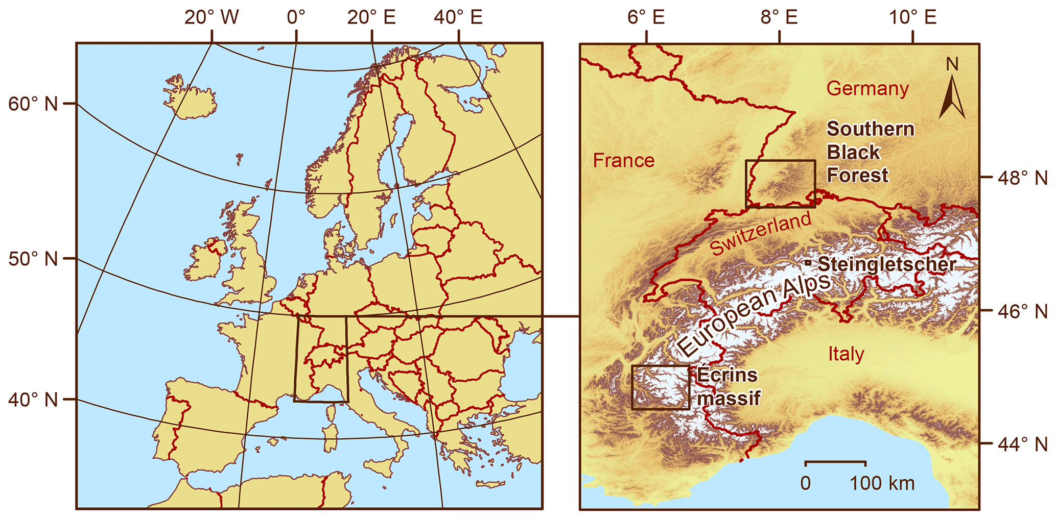
Figure 1 Location of the sites that were chosen for the recalculation of CRE ages. The first site, the Black Forest, lies in the south-western part of Germany close to the border with France and Switzerland. The second site, the Écrins massif, is located in the westernmost European Alps, whereas the third site, the forefield of Steingletscher, is situated in the central Alps further to the north-east. SRTM data (NASA Jet Propulsion Laboratory, 2013) were used to create the map on the right. © EuroGeographics for administrative boundaries.

The southern Black Forest is a low mountainous area, and therefore the result of these experiments may not be representative for high Alpine settings with a rugged relief where many geomorphologists work. To elucidate this issue in further detail, shielding factors for previously dated boulders on Neoglacial moraines in the forefield of a glacier in Switzerland, Steingletscher (Fig. 1; Schimmelpfennig et al., 2014), were calculated. Shielding factors were derived from a light detection and ranging (LiDAR)-based DEM (swissALTI^3D; available at: https://www.swisstopo.admin.ch/de/geodata/height/alti3d.html, last access: 19 May 2022) with a spatial resolution of 0.5 m. To ensure comparability with the shielding factors for the southern Black Forest, this DEM was resampled to x–y resolutions of 1, 12 and 30 m with bilinear interpolation in ArcMap 10.8.1. In addition, shielding factors were computed with SRTM and TanDEM-X elevation data.

The Écrins massif (westernmost Alps; Fig. 1) was chosen as a third site. Moraines in forefield of several glaciers, the Bonnepierre, Etages, Lautaret and Rateau glaciers, have already been dated, and their ages fall into the Neoglacial (Le Roy et al., 2017). As TanDEM-X data did not cover the sites in the Écrins massif, shielding factors were only calculated with SRTM data with an x–y resolution of 30 m.

3.3 Recalculation of CRE ages

To assess the effect of the different methods for deriving shielding factors on CRE ages, CRE ages of 63 sampling surfaces on moraine boulders in the southern Black Forest, in the forefield of Steingletscher and in the Écrins massif were recalculated. Note that CRE ages were not available for 14 boulders in the southern Black Forest that have been selected for this study. Therefore, only 23 CRE ages were recomputed.

CRE ages of boulders on terminal moraines in a formerly glaciated valley (Sankt Wilhelmer Tal) in the southern Black Forest were recalculated to assess the effect of the different methods for calculating topographic shielding factors on CRE ages of boulders in mountains with an intermediate elevation (<1500 m a.s.l.) that have been exposed to cosmic radiation since the Late Pleistocene. See Hofmann et al. (2022) for the description of the study site and the interpretation of the ages.

To test whether the choice of the topographic shielding factor influences CRE ages of surfaces that have been exposed for the last few millennia, CRE ages of boulders in the forefield of four glaciers in the Écrins massif (n=24) were recomputed. Although ¹⁰Be production rates at sampling sites are much higher than in the southern Black Forest due to higher elevation, the in situ accumulated ¹⁰Be concentrations in the sampled boulders are lower due to the relatively short duration of exposure. The ¹⁰Be concentrations in samples from these boulders range from 2800 to 21 800 atoms ¹⁰Be g⁻¹ quartz and are thus much lower than in the boulders in the southern Black Forest. See Le Roy et al. (2017) for a description of the study site and the interpretation of the ages.

As CRE dating has also been applied to terminal moraines of only a few centuries in age (e.g. Schaefer et al., 2009 or Braumann et al., 2020), CRE ages (n=16) of boulders on Little Ice Age (LIA) and post-LIA terminal moraines of Steingletscher (Fig. 1) were also recalculated. See Schimmelpfennig et al. (2014) for a description of the site and the interpretation of the ages. The ¹⁰Be concentration in samples from the boulders vary between 2230 and 12 220 atoms ¹⁰Be g⁻¹ quartz due to short exposure durations.

As only SRTM data covered all sites, CRE ages were first recalculated with SRTM data-based shielding factors and then with field-data-based shielding factors. The cosmic-ray exposure program (CREp; Martin et al., 2017) was chosen for age calculations. The following parameters were chosen: time-dependent “Lm” scaling (Nishiizumi et al., 1989; Lal, 1991; Stone, 2000; Balco et al., 2008), the ERA40 atmosphere model (Uppala et al., 2005), the atmospheric ¹⁰Be-based geomagnetic database of Muscheler et al. (2005), the density of quartz as sample density (2.65 g cm⁻³) and the ¹⁰Be production rate derived from rock samples from the Chironico landslide (southern Switzerland; Claude et al., 2014). If these parameters are chosen in CREp, the ¹⁰Be production rate at sea level and high latitudes amounts to 4.10±0.10 atoms g⁻¹ quartz a⁻¹. The calculator provides CRE ages in kiloyears before 2010 CE rounded to the nearest decade.

3.4 Statistical analysis

The statistical analysis of the output of the toolbox was performed with the R software (version 4.0.5; R Core Team, 2021) and R Studio (version 1.4.1106; RStudio Team, 2021). Relationships between the GIS-based topographic shielding factors and those derived from field measurements were assessed by computing the Pearson product–moment correlation coefficient and the coefficient of determination (R²). Linear models were considered statistically significant when the calculated p value was lower than the common significance level of α=0.05. It should be noted that this common value is a convention and therefore arbitrary. See Dormann (2020) and references therein for further discussion.

4 Results

4.1 Topographic shielding factors for moraine boulders

SRTM data-based shielding factors for moraine boulders in the southern Black Forest, the Écrins massif and in the forefield of Steingletscher (n=77) were strongly correlated with the field-data-based shielding factors (R²=0.89; p<0.05; Fig. 2a). Considering the boulder height during topographic shielding factor calculations led to a slightly stronger agreement (R²=0.90; p<0.05; Fig. 2b).

Figure 2 (a) Shielding factors for moraine boulders in the southern Black Forest, the Écrins massif and in the forefield of Steingletscher determined with SRTM elevation data versus field-data-based shielding factors. Panel (b) is the same as panel (a), but the shielding factors were corrected for the boulder height. For field-data-based shielding factors for boulders in the Écrins massif and in the forefield of Steingletscher, see Le Roy et al. (2017) and Schimmelpfennig et al. (2014), respectively.

4.1.1 Southern Black Forest

SRTM data-based shielding factors were generally consistent with those derived from field data (R²=0.94; p<0.05; Fig. 3a). As can be seen in Fig. 3a, only the shielding factors for the FS-1a, FS-2a and SW-2 boulders did not match. Incorporating the boulder height during shielding factor calculations led to a slightly stronger agreement (R²=0.95; p<0.05; Fig. 3b). The correlation between the TanDEM-X data-based shielding factors and the field-data-based shielding factors was weaker (R²=0.82; p<0.05; Fig. 3c). The discrepancy was largest for the FS-1a, SW-2, SW-9 and WH-1a boulders (Fig. 3c). Incorporating the boulder height led to inconsistent shielding factors for the FS-1a, FS-2a, SW-2, SW-9 and WH-1a boulders (Fig. 3d). Shielding factors determined with the 1 m DEM were most consistent with field-data-based shielding factors (R²=0.97; p<0.05; Fig. 3e, f). The offset between the shielding factors predicted by the linear model and those computed with the calculator of Balco (2018) was largest for the FS-1a, FS-2a and KS-1a boulders and for the FS-1a, FS-2a and SW-2 boulders when the height of the boulders was taken into account, respectively (Fig. 3e, f).

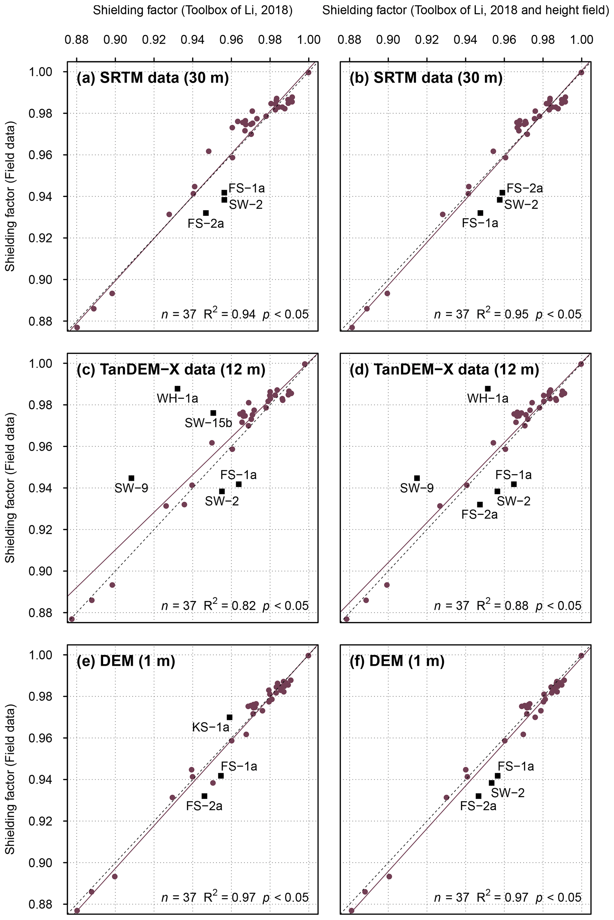
Figure 3 (a) Topographic shielding factors for boulders in the southern Black Forest determined with the ArcGIS toolbox of Li (2018) and SRTM elevation data (NASA Jet Propulsion Laboratory, 2013) versus those derived from field data. Panel (b) is the same as (a), but with a correction for the boulder height. (c) Topographic shielding factors calculated with the ArcGIS toolbox and a TanDEM-X-DEM versus those derived from field measurements. Panel (d) is the same as (c), but the shielding factors were corrected for the boulder height. (e) Topographic shielding factors calculated with the ArcGIS toolbox and the 1 m DEM versus those derived from field measurements. Panel (f) is the same as (e), but with a correction for the boulder height. Outliers are marked with dark red squares. Linear models and 1 : 1 lines are marked with solid and dashed lines, respectively. The numbers in parentheses refer to the spatial resolution of the elevation data.

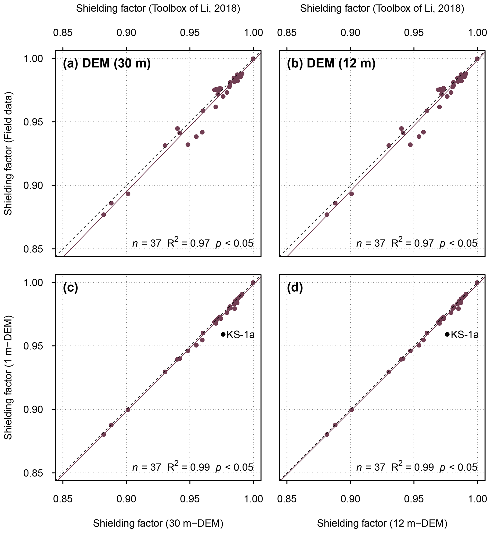
Figure 4 (a) Shielding factors for moraine boulders in the southern Black Forest determined with a resampled version of the 1 m DEM (x–y resolution: 30 m) versus field-data-based shielding factors. (b) Shielding factors determined with a resampled version of the 1 m DEM (x–y resolution: 12 m) versus field-data-based shielding factors. (c) Shielding factors determined with a resampled version of the 1 m DEM (x–y resolution: 30 m) versus those determined with the 1 m DEM. (d) Shielding factors determined with a resampled version of the 1 m DEM (x–y resolution: 12 m) versus those determined with the 1 m DEM.

The correlation between GIS-based and field-data-based shielding factors remained unchanged when resampled versions of the 1 m DEM were chosen as input (R²=0.97; p<0.05; Fig. 4). Only the shielding factors for the KS-1a boulder were different (Fig. 4). For individual shielding factors, see Tables S75 and S76.

4.1.2 Écrins massif

The fit between the GIS-based shielding factors and those derived from field data turned out to be lower than for boulders in the southern Black Forest (R²=0.75; p<0.05; Fig. 5a). Incorporating the boulder height led to a slightly lower agreement (R²=0.74; p<0.05; Fig. 5b). See Table S77 for individual shielding factors.

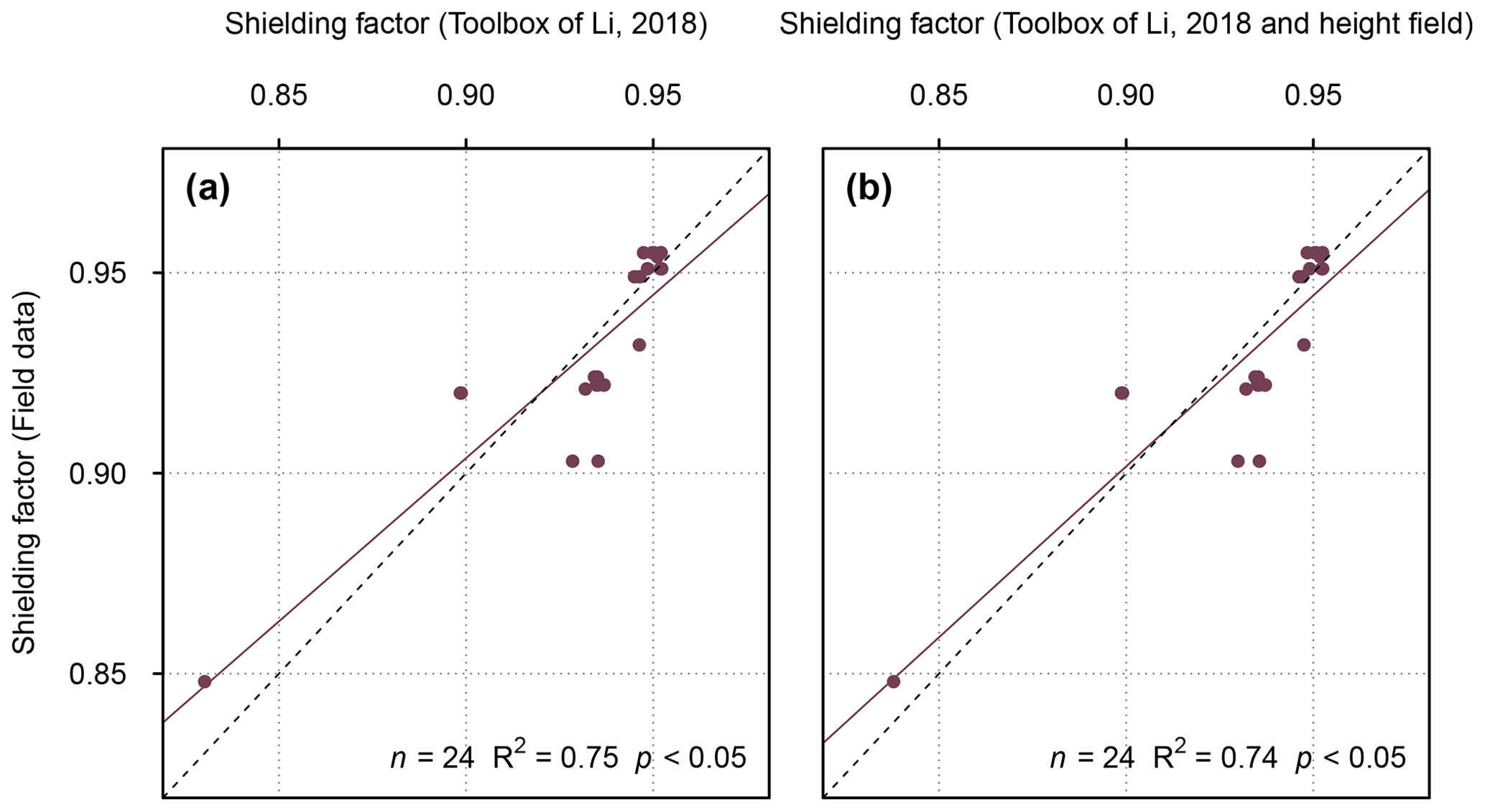
Figure 5 (a) Topographic shielding factors for boulders on moraines in the Écrins massif (Le Roy et al., 2017) derived from field data versus those determined with SRTM elevation data (NASA Jet Propulsion Laboratory, 2013). Panel (b) is the same as (a), but the shielding factors determined with the toolbox are corrected for the boulder height.

4.1.3 Steingletscher

Generally, SRTM data-based shielding factors for moraine boulders in the forefield of Steingletscher were consistent with field-data-based shielding factors (R²=0.70; p<0.05; Fig. 6a, b). The use of TanDEM-X elevation data led to a better fit between the shielding factors (R²=0.78; p<0.05; Fig. 6c, d). After the exclusion of the potentially problematic shielding factors for the STEI-7 boulder, R² rose to 0.91 in both cases (p<0.05).

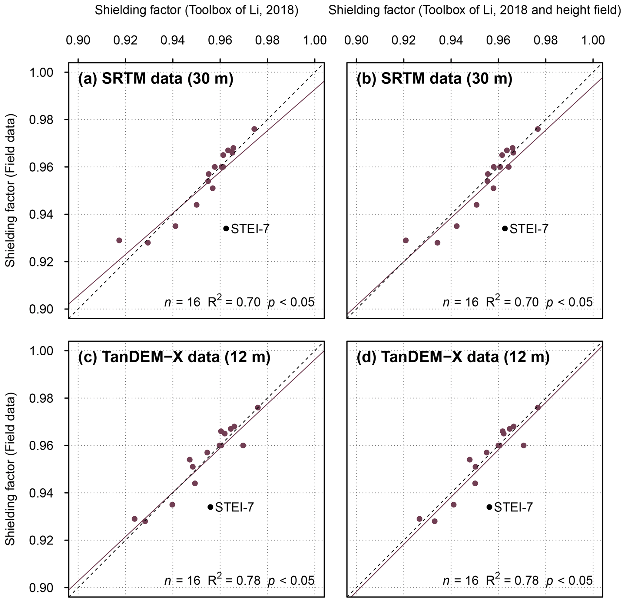
Figure 6 (a) Topographic shielding factors for moraine boulders in the forefield of Steingletscher (Schimmelpfennig et al., 2014) determined with the ArcGIS toolbox and SRTM data versus field-data-based shielding factors. Panel (b) is the same as (a), but the shielding factors were corrected for the boulder height. (c) Topographic shielding factors computed with the toolbox and TanDEM-X elevation data versus field-data-based shielding factors for the same boulders. Panel (d) is the same as (c), but the shielding factors were corrected for the boulder height.

Shielding factors derived from the DEM with an x–y resolution of 1 m (swissALTI^3D) and field-data-based shielding factors were less consistent (R²=0.70; p<0.05; Fig. 7c). The use of resampled versions of the DEM with spatial resolutions of 30 and 12 m led to a similar fit between the shielding factors (R²=0.71 and R²=0.70, respectively; Fig. 7a, b). Irrespective of the input-DEM, GIS-based shielding factors for the STEI-7 boulder did not match the field-data-based shielding factor (Fig. 7). Individual shielding factors are given in the Supplement (Tables S78 and S79).

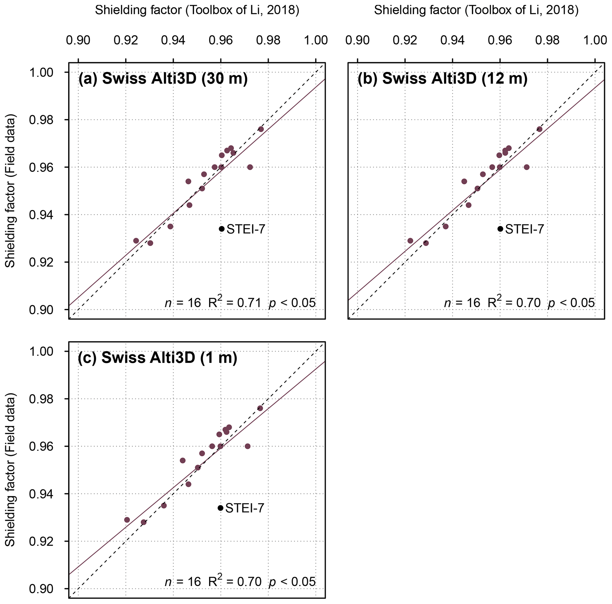
Figure 7 Topographic shielding factors for moraine boulders in the forefield of Steingletscher determined with resampled versions of a LiDAR-based DEM (Swiss ALTI3D) with x–y resolutions of (a) 30, (b) 12 and (c) 1 m.

4.2 Recalculated CRE ages

A histogram of differences in CRE ages for the southern Black Forest is presented in Fig. 8a. See Table A1 in Appendix A for individual CRE ages. CRE ages determined with field-data-based shielding factors differed, on average, by 67 years from CRE ages computed with SRTM data-based shielding factors. With respect to the age determined with field-data-based shielding factors, the CRE age difference was, on average, 0.5 %. The maximum CRE age difference amounted to 280 years or 2.0 % (Fig. 8a and Table B1 in Appendix B). As can be seen in Fig. 8a, the CRE age difference for most of the sampled boulders turned out to be less than 1 %.

Figure 8 Histogram of differences in CRE ages for the (a) southern Black Forest, the (b) the Écrins massif and the forefield of (c) Steingletscher.

The average difference in CRE ages for the Écrins massif amounted to 1.2 % with respect to the CRE age determined with field-data-based topographic shielding factors. CRE ages determined with the shielding factors from field data differed, on average, by 35 years from those computed with the GIS-based shielding factors. The maximum CRE age difference amounted to 4.1 % or 120 years (Fig. 8b and Table B2). For most of the sampled boulders, the CRE age difference amounted to 40 years (1.6 %) or fewer (Fig. 8b). Individual CRE ages are given in Table B2.

The recalculated CRE ages for the forefield of Steingletscher were mostly identical to those computed with field-data-based shielding factors (Fig. 8c). For the STEI-26, STEI-12-14 and STEI-12-07 boulders, the CRE age difference turned out to be 10 years (Table B3). Although the shielding factors for the STEI-7 boulder do not agree, the CRE age of the boulder remained unchanged. See Table A3 for individual CRE ages.

5 Discussion

5.1 Impact of the spatial resolution and quality of elevation data on shielding factors

The vegetation-corrected 1 m DEM and two resampled versions yielded very similar shielding factors for boulders in the southern Black Forest. Similarly, the fit between GIS-based and field-data-based shielding factors for boulders in the forefield of Steingletscher was independent of the x–y resolution of the (resampled) swissALTI^3D DEM. Under the condition that shielding at sampling sites is dominated by the far-field horizon, these results suggest that DEMs with x–y resolutions of a few metres do not have an advantage over DEMs with a spatial resolution of ∼ 30 m.

After the exclusion of the potentially problematic shielding factors for the STEI-7 boulder, SRTM DSM-based and TanDEM-X DSM-based shielding factors were equally consistent with field-data-based shielding factors. The similar fit suggests that TanDEM-X data do not have an advantage over SRTM data. The inspection of the skylines for boulders in the forefield of Steingletscher shows that the use of TanDEM-X data might lead to low-quality shielding factors. The skylines derived from TanDEM-X data did not match the topography represented in the swissALTI^3D DEM (which should more precisely represent the actual terrain surface). Discrepancies have been observed on steep slopes that are not well represented in TanDEM-X elevation data and appear noisy (Fig. 9). The skylines for the STEI-12-04 boulder derived from the swissALTI^3D DEM and SRTM data were consistent. Due to noise, the TanDEM-X data-based skyline for the STEI-12-04 boulder should not be considered realistic (Fig. 9).

Figure 9 Skylines for the STEI-12-04 boulder in the forefield of Steingletscher derived from TanDEM-X data, SRTM data and the swissALTI^3D DEM. The skylines were superimposed on a hillshade derived from TanDEM-X data (© DLR 2021). The contour lines are based on a resampled version of the swissALTI^3D DEM (x–y resolution: 1 m).

The use of elevation data with an x–y resolution of ∼ 30 m requires less computational time. In addition, there is a lower risk that small-scale topographic irregularities in the vicinity of the sampling sites of boulders lead to errors during shielding factor calculations. The example of the SW-2 boulder illustrates that the use of a DEM with an x–y resolution of 1 m might lead to problems: according to the skyline created with the toolbox, the nearby moraine crest apparently induced topographic shielding (Fig. 10). Measuring azimuth and elevation angles at the sampling site on the boulder contradict this assumption (Fig. 11). With about 0.8 m, the x–y uncertainty of the coordinates of the sampling surface on the SW-2 boulder is relatively large. Imprecise x–y coordinates of the sampling surface probably explain the disagreement in Fig. 11. If no topographic obstructions with a size of less than one pixel are situated within a few metres of sampling sites, this issue can be solved by selecting a DEM with a larger x–y resolution (∼ 30 m). Indeed, if a DEM with such a spatial resolution is chosen, imprecise coordinates of sampling sites should be less problematic due to the larger pixel size.

Figure 10 (a) Map of the area around the SW-2 boulder and skylines generated with the skyline function in ArcMap 10.8.1. The shaded relief in the background was derived from SRTM elevation data (NASA Jet Propulsion Laboratory, 2013). (b) Detailed map of the area around the SW-2 boulder. The skyline generated with the high-resolution DEM shows that the intensity of cosmic radiation at the sampling surface on the SW-2 boulder is apparently reduced by the moraine crest. (c) Photo of the SW-2 boulder and of the proximal side of the moraine (photo: Felix Martin Hofmann).

One could argue that the effect of small-scale topographic obstructions is ignored during shielding factor calculations if a DEM with a spatial resolution of ∼ 30 m is selected. Norton and Vanacker (2009) demonstrated that small topographic obstructions may induce partial shielding from cosmic rays. If the distance that cosmic rays penetrate through the topographic anomaly is not significantly higher or even lower than the particle attenuation length, a portion of cosmic rays will travel through the object without any interaction. Supposing that this interaction becomes measurable only if this distance is equivalent or larger than the particle attenuation length, measurable topographic shielding only occurs if the largest distance that cosmic rays penetrate through an obstruction is equivalent to the particle attenuation length (Norton and Vanacker, 2009). Assuming an attenuation length of 160 g cm⁻², the depth at which 63 % of the cosmic rays have been stopped will be 61.5 cm for granite (assumed density: ∼ 2.6  g cm⁻³; Gosse and Phillips, 2001). As recommended here, Norton and Vanacker (2009) advocate the use of elevation data with a larger pixel size (>5 m). Quantifying the effect of small-sized topographic anomalies on topographic shielding factors is not possible here. This would require the development of a new GIS-based tool that takes the dimensions of topographic obstructions into account.

Figure 11 Horizon around the sampling surface on the SW-2 boulder according to SRTM data, the 1 m DEM and field data. Elevation and azimuth angles were computed with the skyline and skytable functions in ArcMap 10.8.1.

5.2 The role of vegetation

As highlighted in Fig. 3b, SRTM DSM-based shielding factors for the FS-1a, FS-2a and FS-3a boulders in the southern Black Forest did not match field-data-based shielding factors. Since the boulders were situated in densely forested areas, measuring pairs of azimuth and elevation angles proved difficult during fieldwork. The horizon around the sampling sites was only partly visible. As the farthest visible points were situated on forested mountains, determining precise elevation angles of the terrain surface turned out to be challenging, and hence the field-data-based shielding factors for these boulders may not be reliable. Figure 3b reveals that the SRTM-based shielding factors for the FS-1a, FS-2a and SW-2 boulders turned out to be systematically higher than the field-data-based shielding factors. This observation raises the question of whether the discrepancy could also be due to the lack of a correction for vegetation cover in SRTM data. This explanation is, however, unlikely: the use of the vegetation-corrected DEM led to similar shielding factors for these boulders (Fig. 3f). Excluding the potentially “problematic” shielding factors for the FS-1a, FS-2a and SW-2 boulders leads to a better fit between the shielding factors (R²=0.98; Fig. C1 in Appendix C).

The TanDEM-X DSM-based shielding factors for the FS-1a, FS-2a, SW-2, SW-9 and WH-1a boulders did not agree with field-data-based shielding factors (Fig. 3d). Except of the SW-9 boulder, these boulders were situated in areas covered by mixed and coniferous forests. As TanDEM-X data are not corrected for vegetation, differing canopy heights and small-sized anomalies in vegetation cover are prone to be misinterpreted as topographic obstructions by the toolbox. The SW-9 boulder, for example, was situated in open grassland close to a coniferous forest. Measuring pairs of azimuth and elevation angles in the field turned out to be straightforward, as the horizon around the boulder was even visible through the nearby coniferous forest. Inspecting the skyline for the SW-9 boulder in ArcMap revealed that the edge of the coniferous forest was misinterpreted as a topographic barrier by the toolbox. Excluding the problematic shielding factors for the FS-1a, FS-2a, SW-2, SW-9 and WH-1a boulders led to a strong correlation with field-data-based shielding factors (R²=0.88; Fig. C1). It should be mentioned that SRTM data were acquired in February 2000, i.e. during the leaf-off period in the Northern Hemisphere, whereas TanDEM-X data were obtained by averaging data from multiple acquisitions. Data collection during the leaf-off period could be one explanation for the better performance of SRTM data.

The fit between the GIS-based shielding factors and those from field data for boulders in the southern Black Forest turned out to be highest when vegetation-corrected elevation data were selected as input data for the toolbox. Therefore, it follows that type of the elevation model, i.e. corrected for vegetation or not, determines the quality of shielding factors for sites in vegetated areas.

5.3 Correcting for the boulder height – does it matter?

Incorporating the boulder height during the computation of topographic shielding factors led to a similar correlation between the shielding factors (Figs. 3f, 4b, d) or further increased the fit (Figs. 2b, 3b, d). Considering the height of the boulders during shielding factor calculations only led to a slightly lower fit between the shielding factors in one case (Fig. 5b). Correcting shielding factors for the boulder height is therefore recommended.

5.4 Impact on CRE ages

Recalculating CRE ages of moraine boulders in the southern Black Forest led, in most cases, to minor changes in CRE ages (<1 %). As these shifts would not influence the interpretation proposed by Hofmann et al. (2022), SRTM data seem to be sufficient to compute shielding factors for sampling sites in flat or low mountainous areas. Interestingly, this recommendation also applies to settings with a more rugged relief. If boulders on landforms of a known age are targeted for establishing production rate reference sites, the use of elevation data with a comparably low spatial resolution could introduce additional errors. The use of SRTM data-based shielding factors instead of field-data-based shielding factors resulted in a more pronounced change in CRE ages of boulders in the Écrins massif. The average CRE age difference amounted to 1.6 %. As can be seen in Table B2, the CRE age difference was highest for the boulders with the youngest CRE ages and amounted up to 4.1 %. The comparably large shift in CRE ages is probably due to the relatively weak correlation between the GIS-based and field-data-based shielding factors (R²=0.74). It remains unclear whether this relatively low fit is due to the low quality of field data or imprecise GIS-based shielding factors. As most of the recalculated CRE ages of boulders on moraines of Steingletscher remained unchanged when GIS-based topographic shielding factors were chosen for CRE age calculations, the choice of the shielding factors does not seem to have a substantial influence on CRE ages if recently exposed surfaces in high Alpine settings are targeted for CRE dating.

5.5 Practical guidelines

If the far-field horizon around sampling sites dominates topographic shielding, DEMs with a spatial resolution of a few metres are not necessary for shielding factor calculations. The use of a combination of a DEM with a very high (∼ 1 m) spatial resolution and low-quality x–y coordinates of sampling sites might lead to invalid shielding factors. Unless there are topographic obstructions within a few metres of sampling sites, a DEM with a lower spatial resolution (∼ 30 m) should be selected. If a vegetation-corrected DEM with a spatial resolution of less than 30 m is available for the site of interest, it should be resampled to an x–y resolution of 30 m prior to shielding factor calculations. If there are obstructions with a size of less than one pixel within a few metres of sampling sites, a terrestrial laser scanning or photogrammetry-based DEM with a spatial resolution of about a decimetre is required for shielding factor calculations. If unavailable, shielding factors should be determined with field data. If a study site is vegetation-covered and a DEM is not available, a DSM with a spatial resolution of ∼ 30 m should be selected (such as a 30 m-SRTM-DSM). Shielding factors should be corrected for the boulder height, as this correction resulted in a similar or better fit with field-data-based shielding factors. TanDEM-X data are only suitable as input data if the site of interest lacks important vegetation cover and if the data are checked for noise. In any case of doubt, skylines should be checked for plausibility.

6 Conclusions

In the validation study of his 2018 toolbox, Li (2018) noted that DEMs with spatial resolutions between 90 and 30 m result in similar shielding factors for boulders. The calculation of shielding factors for boulders in a low mountainous area and a high Alpine setting with a 1 m DEM and two resampled versions yielded consistent shielding factors, thus confirming Li's hypothesis. It is shown that the use of a DEM with x–y resolution 1 m and insufficiently precise x–y coordinates might lead to problems if small-sized topographic obstructions are situated in the vicinity of sampling sites. If the far-field horizon dominates shielding at sampling sites, DEMs with an x–y resolution on the order of 30 m should be preferably used to save computational time and to avoid unnecessary problems associated with small-scale topographic irregularities in the vicinity of sampling sites. Unsurprisingly, the use of vegetation-corrected elevation data allowed for calculating shielding factors that better match field-data-based shielding factors. If vegetation-corrected elevation data are not available for a site, a DSM with a spatial resolution of about 30 m should be chosen. Incorporating the height above ground of the sampling surfaces led to a similar agreement between the shielding factors or further increased the fit, and hence shielding factors should be corrected for the boulder height. Replacing field-data-based shielding factors by SRTM data-based shielding factors during CRE age calculations led, in most cases, to minor shifts in CRE ages (<2 %). Overall, the toolbox of Li (2018) provides a promising approach for calculating topographic shielding factors if suitable elevation data are chosen. Due to the high robustness of the results, the toolbox should therefore be used more widely in the field of geochronology.

Appendix A: Principles of the toolbox of Li (2018) and validation

The toolbox requires at least a point file of the sampling sites (vector) and elevation data (raster). The strike and dip of the sampling surfaces (in degrees), as well as the height above ground of the sampling surfaces (in metres), are optional parameters and can be provided in columns in the attribute table of the point file. The name for the field with the GIS-based topographic shielding factors can optionally be defined before running the toolbox (Fig. A1).

The toolbox first retrieves the elevations of the sampling sites from the input DEM. If provided, the height above ground of the sampling site is added to this elevation. The points are then converted into 3D point features and the calculated elevations of the sampling surfaces serve as z dimensions. The skyline and skyline graph functions in ArcMap are subsequently applied to obtain horizontal and vertical angles that describe the horizon around each point. The skyline function generates a skyline that represents the farthest visible points along the line of sight around a locality (default setting: no maximum distance). The increment of the azimuth angle is set to 1^∘ by default. Hence, 360 pairs of azimuth and elevation angles are obtained. Such a high number is normally not ascertained during fieldwork. If the elevation data are correct, the shielding factors should theoretically be more accurate than those derived from field measurements. The skyline graph function then exports horizontal and vertical angles of the points on the skyline for these azimuth angles.

To take the shielding of a dipping surface into account, the range of azimuths (360^∘) are divided into 1^∘ increments and the elevation angle (θ) is calculated for each azimuth according to the following equation:

$$\begin{array}{}\text{(A1)}& \mathit{\theta }=\arctan \left[\tan {\mathit{\theta }}_{\mathrm{d}}\cos \left(\mathrm{\varnothing }-{\mathrm{\varnothing }}_{\mathrm{s}}\right)\right],\end{array}$$

where θ_d and ∅_s are the dip and strike of the dipping surface, respectively. ∅ is the azimuth. Hence, the approach of Li (2018) is identical to the “skyline.m” MATLAB function implemented in the common topographic shielding calculator of Balco (2018).

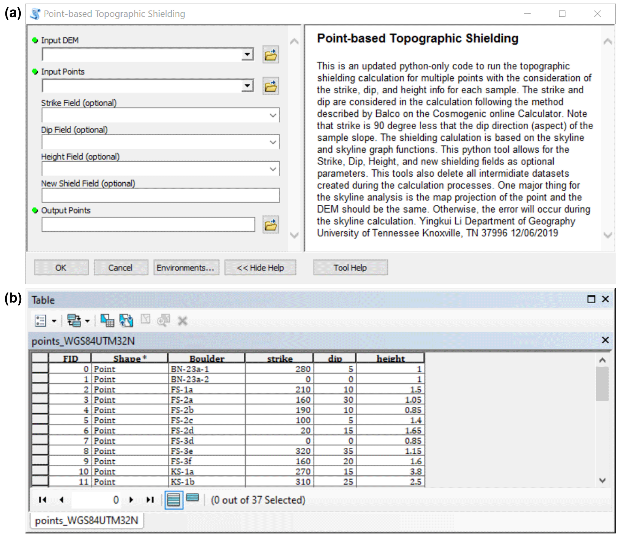
Figure A1 Workflow of toolbox of Li (2018) in the ESRI^® ArcGIS software (Environmental Systems Research Institute, 2020). (a) Screenshot of the graphical interface of the toolbox. The toolbox requires at least a DEM (raster) and a point file of the sampling sites, such as a shapefile. The name of the field in the attribute table with the shielding factors can be specified before running the tool. Strike and dip of the sampled surfaces in degrees and the height above ground of the sampling surfaces in metres need to be inserted in the attribute table of the input points if one wants to correct the shielding factors for these variables. (b) Example of an attribute table of a point file for shielding factor calculations.

The values calculated with Eq. (A1) are compared with the azimuth and elevation angles derived with the skyline and skyline graph functions. Again, this approach is identical to that in the topographic shielding calculator mentioned above. The larger of the two values is used for determining the topographic shielding factor according to the equation of Dunne et al. (1999):

$$\begin{array}{}\text{(A2)}& C_{\mathrm{T}}=\mathrm{1}-{\displaystyle \frac{\mathrm{1}}{\mathrm{2}\mathit{\pi }}}\sum _{i=\mathrm{1}}^n\mathrm{\Delta }{\mathrm{\varnothing }}_i{\sin }^{m+\mathrm{1}}\left({\mathit{\theta }}_i\right),\end{array}$$

where C_T is the topographic shielding factor, n stands for the number of topographic obstructions, ∅_i and θ_i are the azimuth and elevation angles, respectively, associated with each topographic obstruction, and m is an empirical constant. For the latter, an empirical value of 2.3 is commonly used (Nishiizumi et al., 1989; Gosse and Phillips, 2001; Balco et al., 2008).

Li (2018) validated his toolbox by comparing shielding factors computed with his toolbox with shielding factors derived from field measurements for boulders in the Ürümqi catchment in Tian Shan, China. He used SRTM-DSMs with x–y resolutions of 90 and 30 m and the High Mountain Asia 8 m DEM (Shean, 2017) as input elevation data. The topographic shielding factors agree generally with the field-data-based shielding factors (Fig. A2). The use of SRTM data with an x–y resolution of about 30 m resulted in the best fit (Fig. A2b). In addition, he compared the output of his new toolbox with that of an older toolbox (Li, 2013). Both toolboxes yielded similar results (R²=0.84; p<0.05; Fig. A2d).

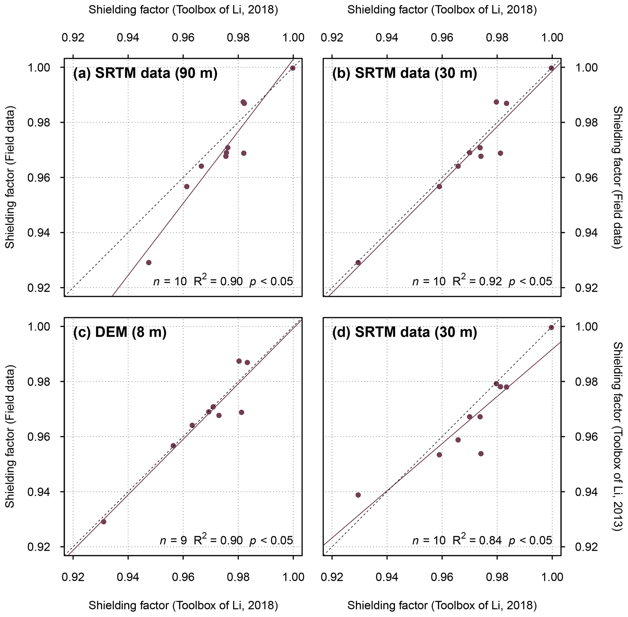
Figure A2 Topographic shielding factors for 10 sampling locations in the Ürümqi catchment in Tian Shan, China, computed with (a) SRTM data, (b) SRTM elevation data with a higher spatial resolution and (c) with the High Mountain Asia DEM (Shean, 2017) versus field-data-based topographic shielding factors. Note that one sampling site is not covered by the High Mountain Asia 8 m DEM, and thus the topographic shielding factor was only determined for nine boulders (Li, 2018). (d) Topographic shielding factors determined with the toolbox of Li (2018) versus the topographic shielding factors derived with an older toolbox (Li, 2013). The strike, dip and height of the sampling surfaces above ground were set to zero in the new toolbox, as the older one does not takes these variables into account (Li, 2018). All correlations are statistically significant when choosing α=0.05 as significance level. The solid and dotted lines are the linear models and 1 : 1 lines, respectively. The numbers in parentheses refer to the spatial resolution of the elevation data. Data from Li (2018).

Appendix B: Recalculated CRE ages

Table B1 CRE ages of boulders on moraines in Sankt Wilhelmer Tal. The ages have already been presented and interpreted elsewhere (Hofmann et al., 2022). They were first calculated with the CREp (Martin et al., 2017) with topographic shielding factors derived from field measurements and then with topographic shielding factors calculated with the ArcGIS-toolbox of Li (2018) and SRTM elevation data (NASA Jet Propulsion Laboratory, 2013).

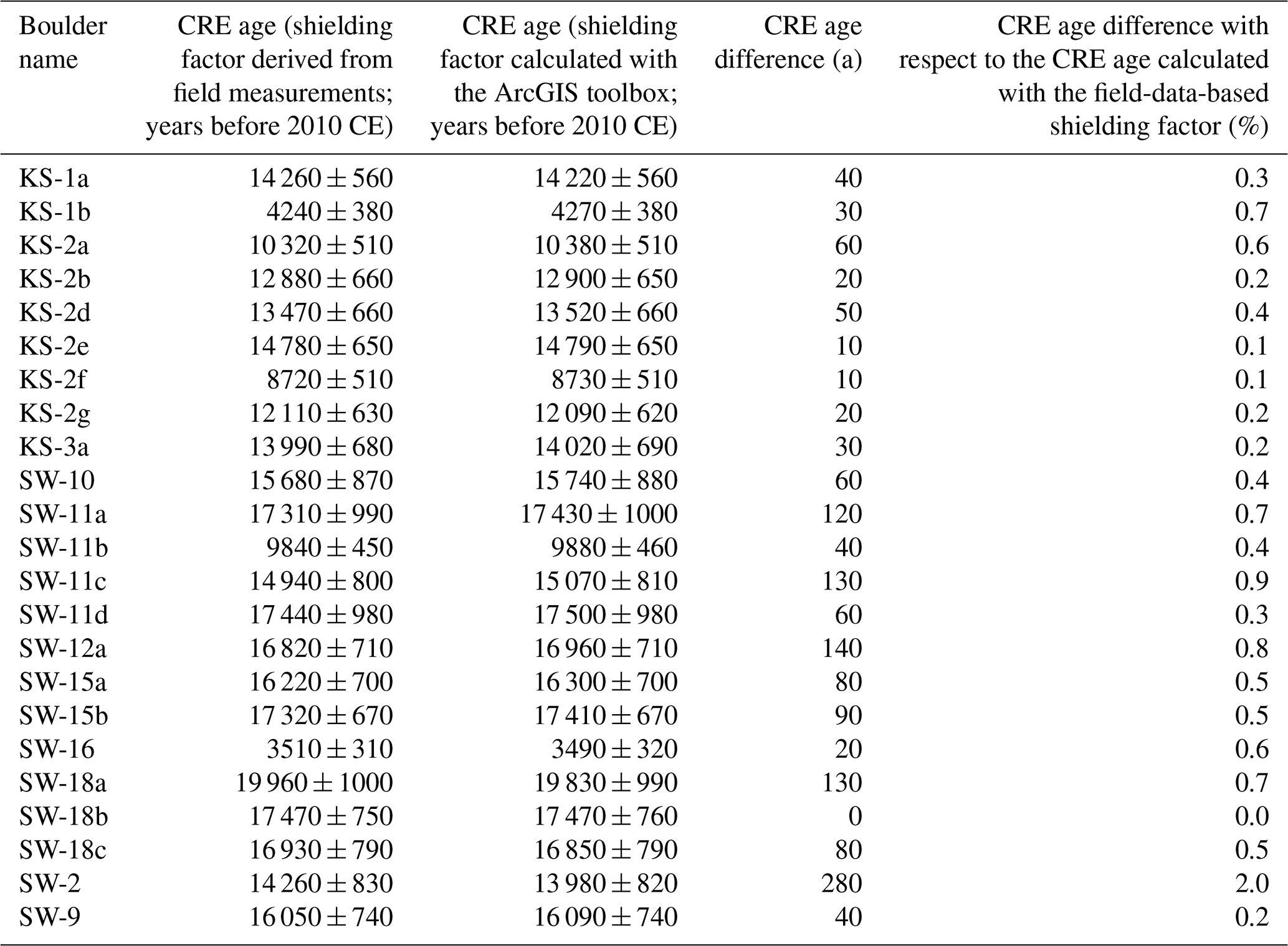
Table B2 Recalculated CRE ages of boulders on terminal moraines of the Rateau (RAT), Lautaret (LAU), Bonnepierre (BON) and Etages (ETA) glaciers in the Écrins massif (Le Roy et al., 2017). In the CREp (Martin et al., 2017), the CRE ages were first calculated with topographic shielding factors derived from field measurements (presented in Le Roy et al., 2017) and subsequently with topographic shielding factors calculated with the ArcGIS-toolbox of Li (2018) and SRTM elevation data (NASA Jet Propulsion Laboratory, 2013).

Table B3 Recalculated CRE ages of moraine boulders in the forefield of Steingletscher (Switzerland; Schimmelpfennig et al., 2014). In the CREp (Martin et al., 2017), CRE ages were first calculated with topographic shielding factors derived from field measurements (presented in Schimmelpfennig et al., 2014) and then with topographic shielding factors calculated with the ArcGIS-toolbox of Li (2018) and SRTM elevation data (NASA Jet Propulsion Laboratory, 2013).

Appendix C: Fit between shielding factors for moraine boulders in the southern Black Forest after the exclusion of outliers

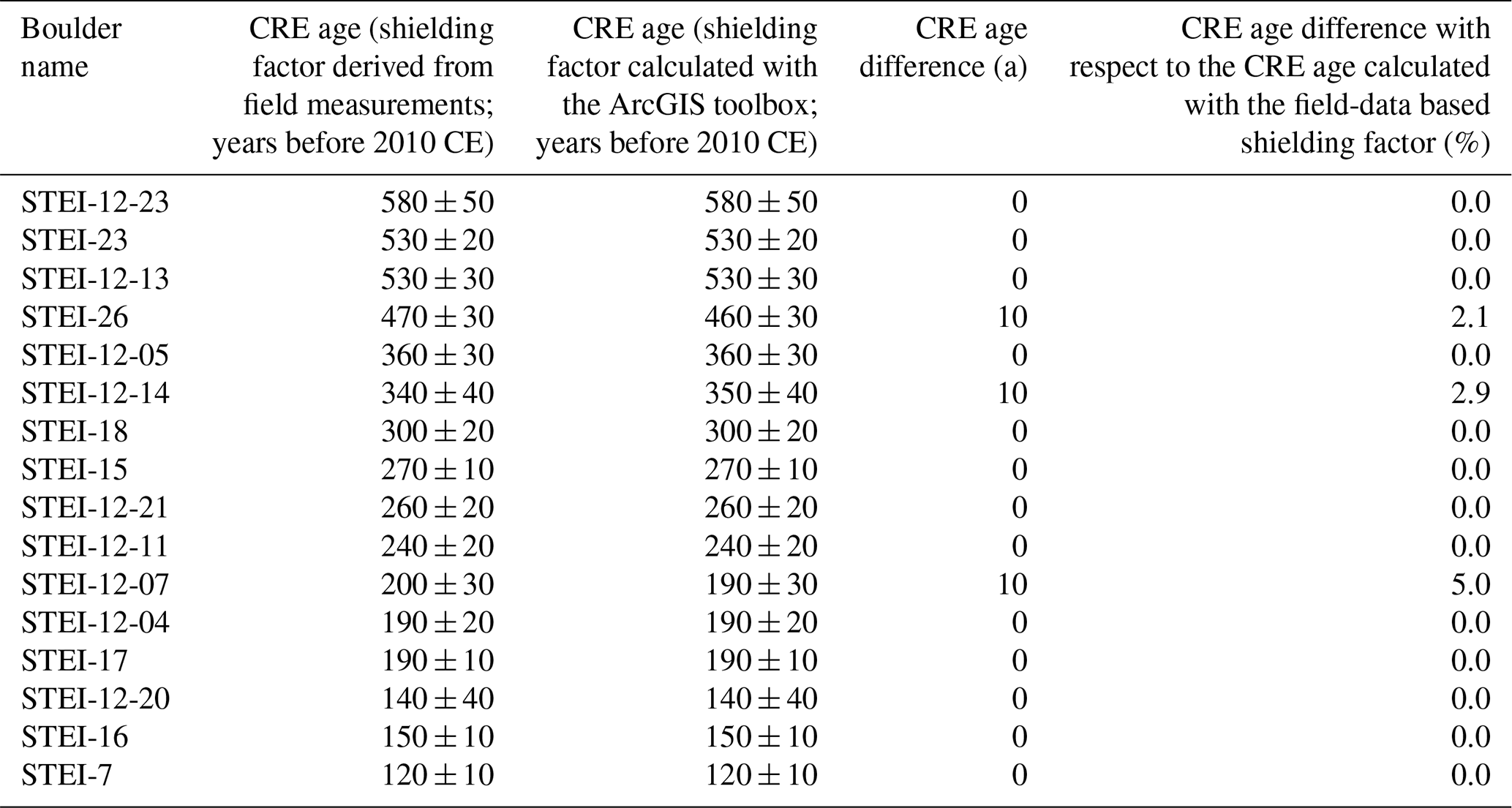
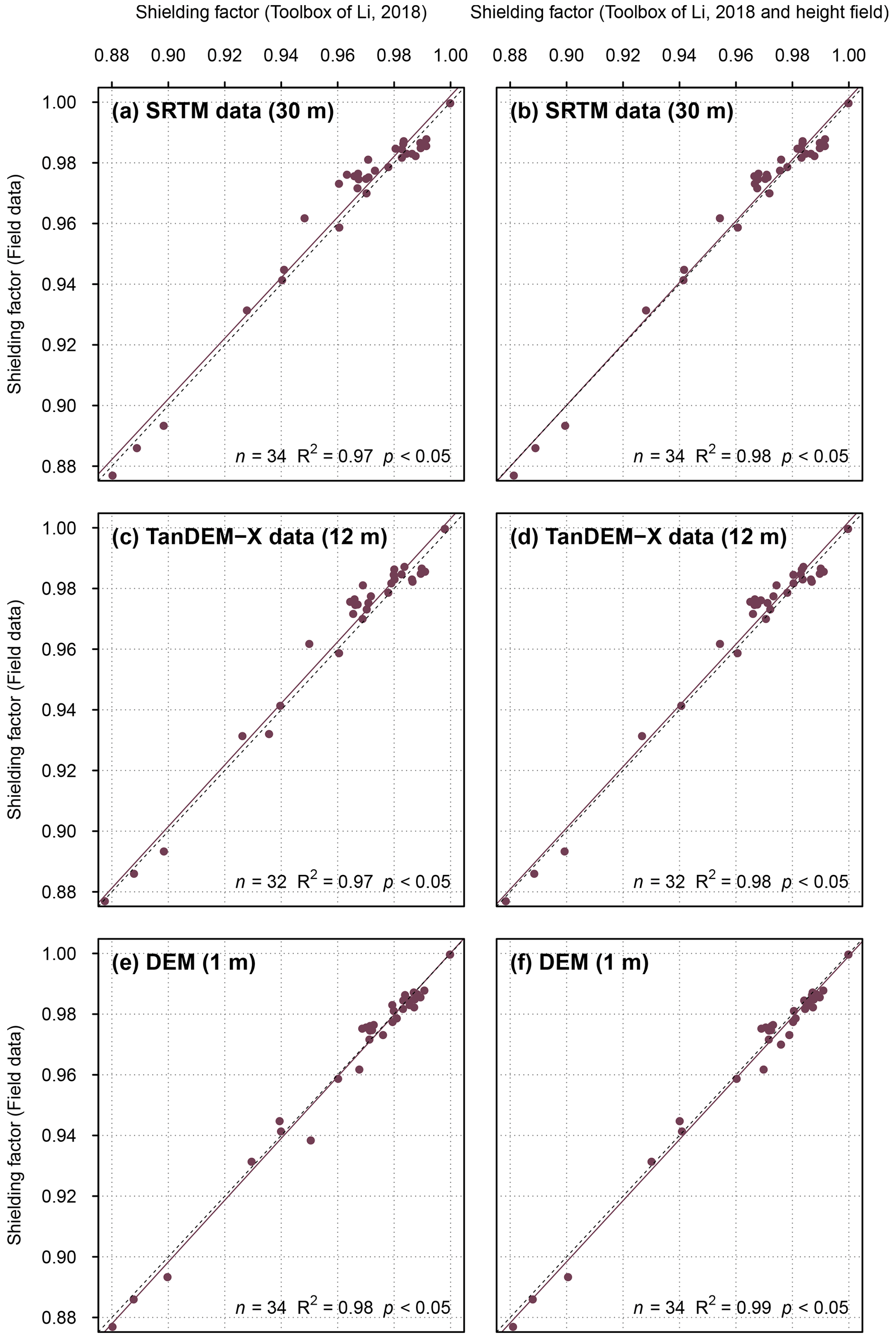
Figure C1 (a) SRTM DSM-based shielding factors versus field-data-based shielding factors. Problematic shielding factors for the FS-1a, FS-2a and SW-2 boulders were excluded from analysis. Panel (b) is the same as (a), but SRTM DSM-based shielding factors were corrected for the boulder height. (c) TanDEM-X DEM-based shielding factors versus field-data-based shielding factors. Problematic shielding factors for the FS-1a, FS-2a and SW-2 boulders were excluded from analysis. Panel (d) is the same as (c), but TanDEM-X DEM-based shielding factors were corrected for the boulder height. (e) Shielding factors determined with the 1 m DEM versus field-data-based shielding factors. Problematic shielding factors for the FS-1a, FS-2a and SW-2 boulders were excluded from analysis. Panel (f) is the same as (e), but GIS-based shielding factors were corrected for the boulder height.