Constraining the aggradation mode of Pleistocene river deposits based on cosmogenic radionuclide depth profiling and numerical modelling

Pleistocene braided-river deposits commonly represent long periods of non-deposition or erosion that are interrupted by rapid and short aggradation phases. When dating these sedimentary sequences with in situ-produced cosmic radionuclides (CRNs), simple concentration depth profiling approaches often fall short, as they assume that the alluvial sedimentary sequence has been deposited with a constant and rapid aggradation rate and been exposed to cosmic radiations afterwards. Numerical modelling of the evolution of CRNs in alluvial sequences permits one to account for aggradation, non-deposition and erosion phases and can simulate which scenarios of aggradation and preservation most likely represent the river dynamics. In this study, such a model was developed and applied to a Middle Pleistocene gravel sheet (Zutendaal gravels) exposed in NE Belgium. The model parameters were optimised to the observed ¹⁰Be and ²⁶Al concentrations of 17 sediment samples taken over a depth interval of 7 m that constitutes the top of a gravel sheet up to 20 m thick. In the studied sedimentary sequence, (at least) three individual aggradation phases that were interrupted by non-deposition or erosion can be distinguished, each interruption lasting ∼ 40 kyr. The age for the onset of aggradation of the upper 7 m of the gravel sheet was further constrained to ${\mathrm{654}}_{-\mathrm{62}}^{+\mathrm{218}}$ ka. This age, within error limits, does not invalidate previous correlations of the gravel sheet with the Cromerian Glacial B and Marine Isotope Stage (MIS) 16. The deposition of the entire gravel sheet likely represents more than one climatic cycle and demonstrates the importance of accounting for the depositional modes of braided rivers when applying in situ cosmogenic radionuclide techniques.

1 Introduction

In situ-produced cosmogenic radionuclides (CRNs, e.g. ¹⁰Be and ²⁶Al) are now widely used to infer erosion rates and exposure time of depositional landforms and allow one to better constrain the long-term landscape evolution of the Quaternary (e.g. Hancock et al., 1999; Schaller et al., 2001; Hidy et al., 2018). To constrain the post-depositional history of fluvial deposits, depth profiles are often used. They consist in measuring the CRN concentration over a depth interval of several metres below the surface. The CRN concentration in the upper 2 to 3 m decreases exponentially with depth, and the shape of the CRN depth profile informs on the average erosion rate and the post-depositional age. Below 3 m, the CRN concentration asymptotically decreases to a value that is assumed to represent the CRNs conserved from previous exposure episodes, the pre-depositional inheritance (e.g. Siame et al., 2004; Braucher et al., 2009; Hidy et al., 2010).

Measured CRN concentrations can then be fitted to numerical model predictions via an optimisation process. A minimum of five samples from the same, undisturbed sedimentary sequence is often necessary to obtain reliable results for exposure and erosion rates (Braucher et al., 2009; Hidy et al., 2010; Laloy et al., 2017). The depth profile technique assumes that the aggradation process is continuous and negligible in duration compared to the post-depositional exposure and that the inheritance is negligible or constant (Braucher et al., 2009; Laloy et al., 2017). Successful applications of CRNs to date Quaternary deposits include (glacio)fluvial terraces (e.g. Rixhon et al., 2011, 2014; Xu et al., 2019), alluvial fans (e.g. Rodés et al., 2011) or glacial moraines (e.g. Schaller et al., 2009) that underwent negligible or constant erosion rates over the time of exposure (Braucher et al., 2009).

Depositional sequences can show discontinuous aggradation modes, limiting the applicability of classical CRN depth profiling. Examples exist of Pleistocene river deposits that consist of several sedimentary cycles (Mol et al., 2000; Vandenberghe, 2001; Lauer et al., 2010, 2020; Vandermaelen et al., 2022a). Between the aggradation of each sequence lies a potential phase of landscape stability or erosion, hereafter referred to as a hiatus. While short hiatuses in the deposition process are, in principle, undetectable from a depth profile, recent work by e.g. Vandermaelen et al. (2022a) showed that > 5000 years-long hiatuses leave a clear imprint on the CRN depth profile. Further development of the classical depth profile technique is necessary to account for multiple aggradation phases and modes when constraining the history of depositional landforms like braided-river deposits (Nichols et al., 2002, 2005; Balco et al., 2005; Dehnert et al., 2011; Rixhon et al., 2011, 2014; Rizza et al., 2019).

In this study, we evaluate whether it is possible to reconstruct the aggradational mode of Pleistocene braided-river deposits based on in situ-produced CRN data collected over a ∼ 7 m thick sedimentary sequence. We developed a numerical model that simulates the accumulation of cosmogenic radionuclides, ¹⁰Be and ²⁶Al, in a sedimentary sequence and that accounts for deposition and erosion phases and post-depositional exposure. The model is applied to Pleistocene gravel deposits, the Zutendaal gravels. The 7 to 15 m thick gravel sheets of the Zutendaal Formation are found in NE Belgium and are assumed to be of Middle Pleistocene age (Paulissen, 1983; Gullentops et al., 2001; Beerten et al., 2018). The thickness of the deposits, availability of geochemical proxy data and good preservation make them an excellent candidate for this study on complex aggradation modes.

2 Material and methods

2.1 Accumulation of CRN over time

2.1.1 Principles of numerical model

The model simulates the buildup of (i) a sedimentary sequence, including phases of aggradation, non-deposition and erosion, and (ii) the in situ-produced cosmogenic radionuclide concentrations in the sedimentary column. The exposure time of the sequence corresponds to the time elapsed since the onset of the deposition (i.e. aggradation) of the oldest, bottommost layer. The model treats the exposure time as the sum of a discrete number of time periods of variable duration (kyr) (Fig. 1). During a time period, there is either deposition of sediments with a given thickness (cm) on top of the pre-existing column (aggradation phase), surface erosion of a given amount of sediments (cm) (erosion phase) or landscape stability (no addition nor removal of sediments). The model allows one to specify the lower and upper bounds of the duration of the time periods and the amount of aggradation or erosion. A time period characterised by either stability or erosion can be defined to represent not only an interruption in the aggradation process but also the (often much longer) post-depositional time. In the following sections, the total length of all aggradation, erosional or stable phases is referred to as the “total formation time (kyr)”, whereas the period of time after abandonment is cited as the “post-depositional time (kyr)”. The sum of the two thus represents the exposure time (kyr).

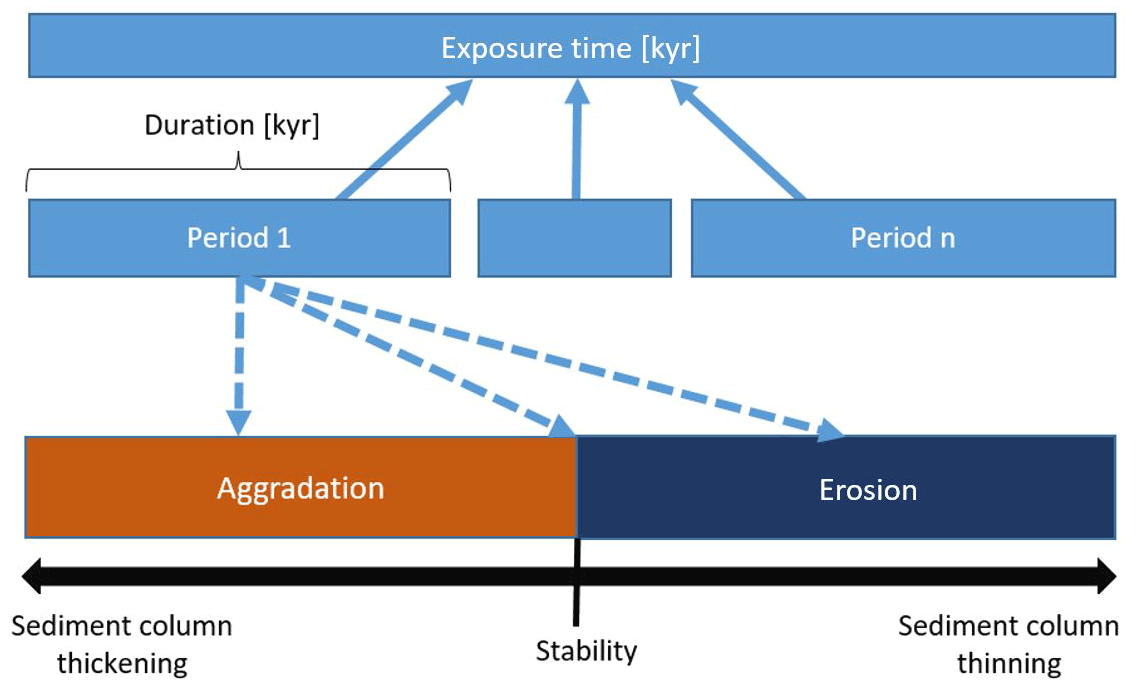
Figure 1 Structure of the model. The total exposure time is divided in a number of time periods, during which the sediment column is building up (aggradation phase), eroding (erosion phase) or not changing (stability).

The functioning of the model is exemplified in Fig. 2, where an example is given for the buildup of a sedimentary column in three phases. During the first time period, T1, from t₀ until t₁, the deposition starts during an aggradation phase. Aggradation is then interrupted by an erosion phase of duration T2, lasting from t₁ until t₂. After erosion, a new aggradation phase of duration T3 occurs between t₂ and t₃. After that, the fluvial sequences are abandoned and preserved until now, i.e. the end of the exposure time. The depth variation of in situ-produced cosmogenic radionuclides in the sedimentary sequence shows the effect of the complex aggradation history (Fig. 2) with two superimposed CRN depth profiles. The lower CRN depth profile developed between t₀ and t₁ and was truncated during the erosion phase of T2. If the profile was buried at great depth (typically > 10 m) and shielded from cosmic rays, no further accumulation of CRN occurred after t₂. The upper CRN depth profile developed since the onset of the T3 aggradation phase, and the buildup of CRN continued after abandonment of the sequence. Such a discontinuous aggradation mode creates a CRN concentration depth profile that cannot properly be explained by model descriptions of classical “simple” CRN depth profiles.

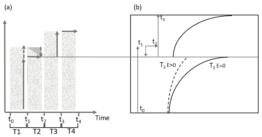
Figure 2 Illustration of the effect of discontinuous aggradation on the depth profile of cosmogenic radionuclide concentrations. (a) The sedimentary sequence consists of two aggradation phases (T1 and T3) that are interrupted by erosion or stability during T2. (b) The in situ-produced CRN profile shows two superimposed classical CRN depth profiles. The lower part of the profile represents two depth profiles: the dashed line illustrates the CRN depth profile when T2 undergoes erosion (E > 0), and the solid line represents the CRN depth profile when T2 corresponds to a stability phase (E = 0).

2.1.2 Model equations

The production rate of in situ cosmogenic radionuclides at a given depth, z (cm), in a sedimentary deposit can be described as follows:

$$\begin{array}{}\text{(1)}& P_i\left(z\right)=P_i\left(z_{\mathrm{0}}\right)\cdot e^{\left(\frac{-z\cdot \mathit{\rho }}{{\mathrm{\Lambda }}_i}\right)}.\end{array}$$

P_i(z₀) (in atoms per gram of quartz per year, later referred to as at. g${}_{\mathrm{qtz}}^{-\mathrm{1}}$ yr⁻¹) is the production rate of CRN (¹⁰Be or ²⁶Al) at the surface, z=z₀ (cm), via the production pathway i, denoting either spallation by neutrons or capture of fast or negative muons. The attenuation length, Λ_i (g cm⁻²), is a measure of the attenuation of CRN production with depth and was set to 160, 1500 and 4320 g cm⁻² for the production by, respectively, neutrons, negative muons and fast muons (Braucher et al., 2011). The dry bulk density of material is written as ρ (g cm⁻³). The model predefines the sea level high-latitude (SLHL) production rate for ¹⁰Be at 4.25 ± 0.18 at. g${}_{\mathrm{qtz}}^{-\mathrm{1}}$ yr⁻¹ (Martin et al., 2017), and the value is then scaled based on latitude and altitude of the site, following Stone (2000). The relative spallogenic and muogenic production rates are based on the empirical muogenic-to-spallogenic production ratios established by Braucher et al. (2011), using a fast-muon relative production rate at SLHL of 0.87 % and slow-muon relative production rate at SLHL of 0.27 % for ¹⁰Be and, respectively, 0.22 % and 2.46 % for ²⁶Al.

The CRN concentration changes as function of time and depth, following Dunai (2010):

$$\begin{array}{}\text{(2)}& \begin{array}{rl}C\left(z,t\right)=& C_{\mathrm{inh}}\cdot e^{-\mathit{\lambda }\cdot t}+\sum _i{\displaystyle \frac{P_i\left(z\right)}{\mathit{\lambda }+\frac{\mathit{\rho }\cdot \mathit{\epsilon }}{{\mathrm{\Lambda }}_i}}}\cdot e^{-\frac{\mathit{\rho }\cdot \left(z_{\mathrm{0}}-\mathit{\epsilon }\cdot t\right)}{{\mathrm{\Lambda }}_i}}\\ & \cdot \left(\mathrm{1}-e^{-\left(\mathit{\lambda }+\frac{\mathit{\rho }\cdot \mathit{\epsilon }}{{\mathrm{\Lambda }}_i}\right)\cdot t}\right),\end{array}\end{array}$$

where C_inh (at. g${}_{\mathrm{qtz}}^{-\mathrm{1}}$) is the concentration of inherited CRNs from previous exposure before or during transport to the final sink, λ (yr⁻¹) is the nuclide decay constant, and ε is the erosion rate (cm yr⁻¹). We used a half-life of 1387 kyr for ¹⁰Be (Korschinek et al., 2010; Chmeleff et al., 2010) and 705 kyr for ²⁶Al (Nishiizumi, 2004).

The model simulates the CRN concentrations during the buildup of a sedimentary column and considers phases of aggradation, stability and erosion. The model is discretised in 1 cm depth slices. The aggradation or erosion rate (cm yr⁻¹) is obtained by dividing the total thickness of the sediments deposited or eroded during one sedimentary phase by the duration of the phase. Then, the model calculates the corresponding thickness (cm) of the layer to be aggraded or removed per aggradation or erosion phase as a function of the aggradation or erosion rate. Aggradation phases are discretised in time steps of 1 kyr. The thickness of material to be aggraded is distributed equally over each time step of the aggradation phase. When the value is not discrete, the model keeps track of the remaining values and adds them to the thickness to be aggraded over the next time step. For every centimetre added on top of the column, the depth values are dynamically adjusted and change from z to z+1. Compared to earlier work by, e.g. Nichols et al. (2002) or Rizza et al. (2019), the advantage of our approach is the flexible setup of the model, whereby the user can tune the model complexity and its parameters easily as to adapt it to a specific study case.

At each time step, the concentrations of ¹⁰Be and ²⁶Al along the depth profile are dynamically adjusted, taking into account the production or removal of CRNs during each phase (erosion or stability) or time step. The inherited and the in situ-produced CRN concentrations are corrected for the natural decay of ¹⁰Be and ²⁶Al as a function of the remaining exposure time. The radioactive decay of CRNs becomes important for Middle to Late Pleistocene deposits and is explicitly accounted for, in contrast to earlier work by e.g. Nichols et al. (2002, 2005). The ²⁶Al and ¹⁰Be in situ production rates and the inherited concentrations are predefined in the model. By default, the model assumes that all sediments arrive in their final sink with an inherited ²⁶Al $/$ ¹⁰Be ratio equal to the surface production ratio which is set at 6.75 (Nishiizumi, 1989; Balco and Rovey, 2008; Margreth et al., 2016). The ²⁶Al $/$ ¹⁰Be ratio of the inherited CRNs can be adjusted in the model to allow for simulations with a ²⁶Al $/$ ¹⁰Be production ratio of 8.0 to 8.4 at depth, as reported by Margreth et al. (2016) and Knudsen et al. (2019). Such simulations could then represent the aggradation of material that is sourced by deep erosion by, e.g. (peri)glacial processes (Akçar et al., 2017; Claude et al., 2017).

2.1.3 Fitting model outputs to ¹⁰Be and ²⁶Al observed data

We used the reduced χ² value as the optimisation criterion. The null hypothesis stipulates that the probability of finding a χ² value higher than the one that we measure is likely. In that case, the expected distribution cannot be rejected and is conserved as a possible solution. After each model simulation, the reduced χ² value (Taylor, 1997) is derived following Eq. (3):

$$\begin{array}{}\text{(3)}& {\mathit{\chi }}^{\mathrm{2}}={\displaystyle \frac{\mathrm{1}}{d}}\sum _{i=\mathrm{1}}^n{\left({\displaystyle \frac{\left(Y_i^{\mathrm{obs}}-Y_i^{\mathrm{mod}}\right)}{{\mathit{\sigma }}_i}}\right)}^{\mathrm{2}},\end{array}$$

where $Y_i^{\mathrm{obs}}-Y_i^{\mathrm{mod}}$ is the difference between observed and modelled ²⁶Al and ¹⁰Be concentrations; σ_i is the standard error encompassing all process and analytical errors, and d corresponds to the degrees of freedom of the dataset that is equal to the number of observations less the number of unconstrained model parameters. For each simulation, the measured reduced χ² and its associated probability of finding a reduced χ² of higher value is reported. The null hypothesis was rejected at 0.05 significance level, and the parameters of the associated simulation are stored as possible solutions.

2.2 Study area

We selected a study site in the Zutendaal gravels, a fluvial deposit covering the western part of the Campine Plateau (Fig. 3a). The Campine Plateau is a relict surface standing out of the otherwise-flat Campine area, a characteristic lowland of the European Sand Belt. This landscape is primarily a result of periglacial, fluvial and aeolian processes related to glacial–interglacial climatic cycles that took place during the Pleistocene (Vandenberghe, 1995). It is bordered in the east by the terrace staircase of the Meuse Valley and in the northeast by tectonic features, the Feldbiss Fault Zone and the Roer Valley Graben (Fig. 3b). In the southwest, the Campine Plateau is bordered by a cryopediment shaping the transition to the Scheldt basin (Beerten et al., 2018, and references therein).

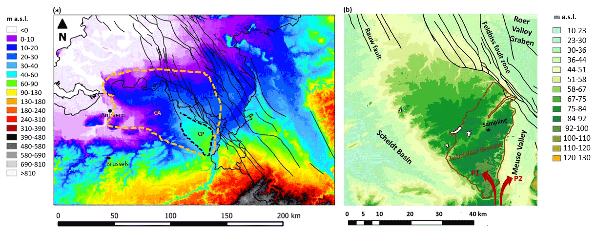
Figure 3 (a) Location of the Campine Plateau (black dashed line) in the low-lying region of the Campine area (CA, delineated by an orange dashed line) on a DTM (digital terrain model; U.S. Geological Survey's EROS Data Center: GTOPO30, 1996), with indications of main faults (Deckers et al., 2014). The whole area belongs to the sandy lowlands of the European Sand Belt. The Campine Plateau stands out of its environment by > 50 m. (b) The Zutendaal gravels (delineated with a brown line) cover the southeastern region and the most elevated parts of the plateau (DTM from GDI-Vlaanderen, 2014). They were deposited by the Meuse River by the time it was flowing westward (red arrow, P1). Later on, this course was abandoned as the Meuse River moved eastward to form the present-day Meuse Valley (red arrow, P2).

The Zutendaal gravels were deposited by the Meuse River during the course of the Early and/or Middle Pleistocene (Beerten et al., 2018; Fig. 3b). By this time, the region corresponded to a wide and shallow river valley occupied by braided-river channels (De Brue et al., 2015; Beerten et al., 2018, and references therein). The Zutendaal gravels are structured as superposed units that possibly represent different aggradation phases related to various deposition modes of braided rivers (Paulissen, 1983; Vandermaelen et al., 2022a). Architectural elements that support the existence of individual aggradation phases include gravel bars and bedforms, channels, sediment gravity flows and overbank fines (Dehaen, 2021). Such an assemblage approaches the structure of shallow gravel-bed braided rivers, defined as Scott-type fluvial deposits by Miall (1996), but has an unusual presence of clay plugs. After deposition of the gravels, the Campine area was subject to erosion (Beerten et al., 2013; Laloy et al., 2017). The erosion-resistant cap of gravel deposits played an important role in the Quaternary landscape evolution of the Campine area: the Zutendaal gravels are now observed at the highest topographic position in the Campine landscape as result of relief inversion (Beerten et al., 2018), whereby the gravel sheet has been covered by wind-dominated Weichselian sands of the Opgrimbie Member, Gent Formation (Beerten et al., 2017). Optically stimulated luminescence dating indicates an age range between ca. 23 and ca. 11 ka, covering the Late Pleniglacial and Late Glacial (MIS 2, Marine Isotope Stage; Derese et al., 2009; Vandenberghe et al., 2009).

The age control on aggradation and post-depositional erosion is poor, but the onset of aggradation is commonly assumed not to be older than 1000 ka (van den Berg, 1996; Van Balen et al., 2000; Gullentops et al., 2001; Westerhoff et al., 2008). The onset of post-depositional erosion remains unknown, but post-depositional erosion did not start before 500 ka (van den Berg, 1996; Van Balen et al., 2000; Westerhoff et al., 2008). The specific duration and mode of aggradation of the Zutendaal gravels remain currently unresolved.

2.3 Sampling and laboratory treatment

We sampled an abandoned gravel pit at the geosite “Quarry Hermans” (Bats et al., 1995) in As (51^∘00^′29.10^′′ N, 5^∘35^′46.19^′′ E, Fig. 3), where the Zutendaal gravels are exposed over a thickness of about 7 m. At least a comparable thickness of the Zutendaal gravels is supposed to be present underneath the exposure. The gravel sheet is covered by 60 cm of coversands, whereby the top of the profile reaches an altitude of 85 m a.s.l. The section was described in the field, with annotations of grain size and sorting, sedimentary structures, and traces of chemical weathering, including oxidation (Vandermaelen et al., 2022a). These observations allowed the subdivision of the profile into six units (U1–U6, Fig. 4). Over the depth range of 70–660 cm, we took 37 bulk samples for grain size and bulk elemental analyses. Seventeen samples were processed for in situ-produced CRN analyses: 14 for ¹⁰Be to construct a depth profile and 3 for ²⁶Al to analyse the ²⁶Al $/$ ¹⁰Be ratio in the main sedimentological units of the profile. Given that the uncertainties on ²⁶Al quantifications are larger than those for ¹⁰Be because of the necessity to perform additional measurements of stable ²⁷Al on Inductively Coupled Plasma Atomic Emission Spectroscopy (ICP-AES), the number of ¹⁰Be samples outnumbers the ²⁶Al samples.

Figure 4 Field observations used to constrain simulations. The log illustrates six units, labelled from U1 to U6, that were defined based on grain size, contact geometry, sedimentary structure, sorting and weathering traces observed in the field. The maximum grain size of the units is shown on the top x axis (C: clay, Si: silt, VFS: very fine sand, FS: fine sand, MS: medium sand, CS: coarse sand, VCS: very coarse sand, VFG: very fine gravel, MG: medium gravel, CG: coarse gravel, VCG: very coarse gravel). They are covered by Weichselian, aeolian coversands (abbreviated UWS). U1, U3 and U4 present imbrication and represent crudely bedded gravels (Gh). U2, U5 and U6 represent horizontally bedded sands (Sh) or pebbly fine to very coarse sands (Sp). The granulometry is illustrated by the D50 (black line), and the limits of the shaded area define the D10 on the left and the D90 on the right of the black line. Panels (a)–(d) represent illustrations of the different units. Panels (e)–(f) represent very coarse gravels collected in U1 showing Mn coatings. Panel (g) illustrates weathered gravels from U3 showing Fe coatings.

Samples were processed for in situ cosmogenic ¹⁰Be and ²⁶Al analyses, following Vanacker et al. (2007, 2015). Samples were washed, dried, and sieved, and the 500–1000 µm grain size fraction was used for further analyses. Chemical leaching with a low concentration of acids (HCl, HNO₃ and HF) was applied to purify quartz in an overhead shaker. Later on, purified samples of 10–40 g of quartz were leached with 24 % HF for 1 h to remove meteoric ¹⁰Be. This was followed by spiking the sample with ⁹Be and by total decomposition in concentrated HF. About 0.200 mg of ⁹Be was added to samples and blanks. The beryllium in the solution was then extracted by ion exchange chromatography, as described in von Blanckenburg et al. (1996). Three laboratory blanks were processed.

The ¹⁰Be $/$ ⁹Be and ²⁶Al $/$ ²⁷Al ratios were measured using accelerator mass spectrometry on the 500 kV Tandy facility at ETH Zurich (Christl et al., 2013). The ¹⁰Be $/$ ⁹Be ratios were normalised with the in-house standard S2007N and corrected with the average ¹⁰Be $/$ ⁹Be ratio of three blanks of (1.3 ± 0.6) × 10⁻¹⁴. The analytical uncertainties on the ¹⁰Be $/$ ⁹Be ratios of blanks and samples were then propagated into the 1 standard deviation analytical uncertainty for ¹⁰Be concentrations. We then plotted the ¹⁰Be concentrations and their respective uncertainties as functions of depth below the surface.

We measured the ²⁷Al concentrations naturally present in the purified quartz by inductively coupled plasma-atomic emission spectroscopy (Thermo Scientific iCAP 6000 Series) at the MOCA platform of UCLouvain in Louvain-la-Neuve, Belgium. The ²⁶Al $/$ ²⁷Al results measured at ETH Zurich were calibrated with the nominal ²⁶Al $/$ ²⁷Al ratio of the internal standard ZAL02, equal to (46.4 ± 0.1) × 10⁻¹². We subtracted from each measurement a ²⁶Al $/$ ²⁷Al background ratio of (7.1 ± 1.7) × 10⁻¹⁵ (Lachner et al., 2014). We reported analytical uncertainties with 1 standard deviation, including the propagated error of 24 % coming from the background, the uncertainty associated with AMS counting statistics, the AMS external error of 0.5 % and the 5 % stable ²⁷Al measurement (ICP-AES) uncertainty. The accuracy of the element chemistry was tested with reference material BHVO-2, and the analytical uncertainty was evaluated at < 3 % for major element concentrations and < 6 % for trace element concentrations (Schoonejans et al., 2016).

2.4 Scenarios to constrain the geomorphic history of fluvial deposits

We implemented four scenarios in our model. Each scenario consists of a succession of “n” time periods, referred to as Ti, that correspond to the interval [t_i−1, t_i], with i representing the limits of a time period in the geomorphic history. Parameters are listed in Table 1. The periods are characterised by a single geomorphic setting (i.e. E is erosion, A is aggradation, S is stability), whereby a given thickness of sediment is removed or aggraded (cm) over a certain time interval (kyr). Durations and thicknesses are sampled from a uniform distribution, whose upper and lower bounds are stated between square brackets in Table 1. Inheritance parameters were sampled from a normal distribution (with mean and standard deviation reported in Table 1) that is centred on the inheritance that was reported in previous studies on Quaternary Meuse deposits (Rixhon et al., 2011; Laloy et al., 2017). A uniform bulk density of 2.1 g cm⁻³ was used, based on bulk density measurements of 17 samples. The four scenarios are summarised in Fig. 5.

Table 1 Description of four scenarios that are used to constrain the geomorphic history of fluvial deposits. The different periods are presented in the headers. Each period is characterised by aggradation (A), stability (S) or erosion (E); a specific duration; a thickness to aggrade or remove; and an inherent concentration. When uniform distributions are used, the lower and upper bounds of the interval are given between square brackets. When values are depicted in a normal distribution, the mean and standard deviation are given between round brackets.

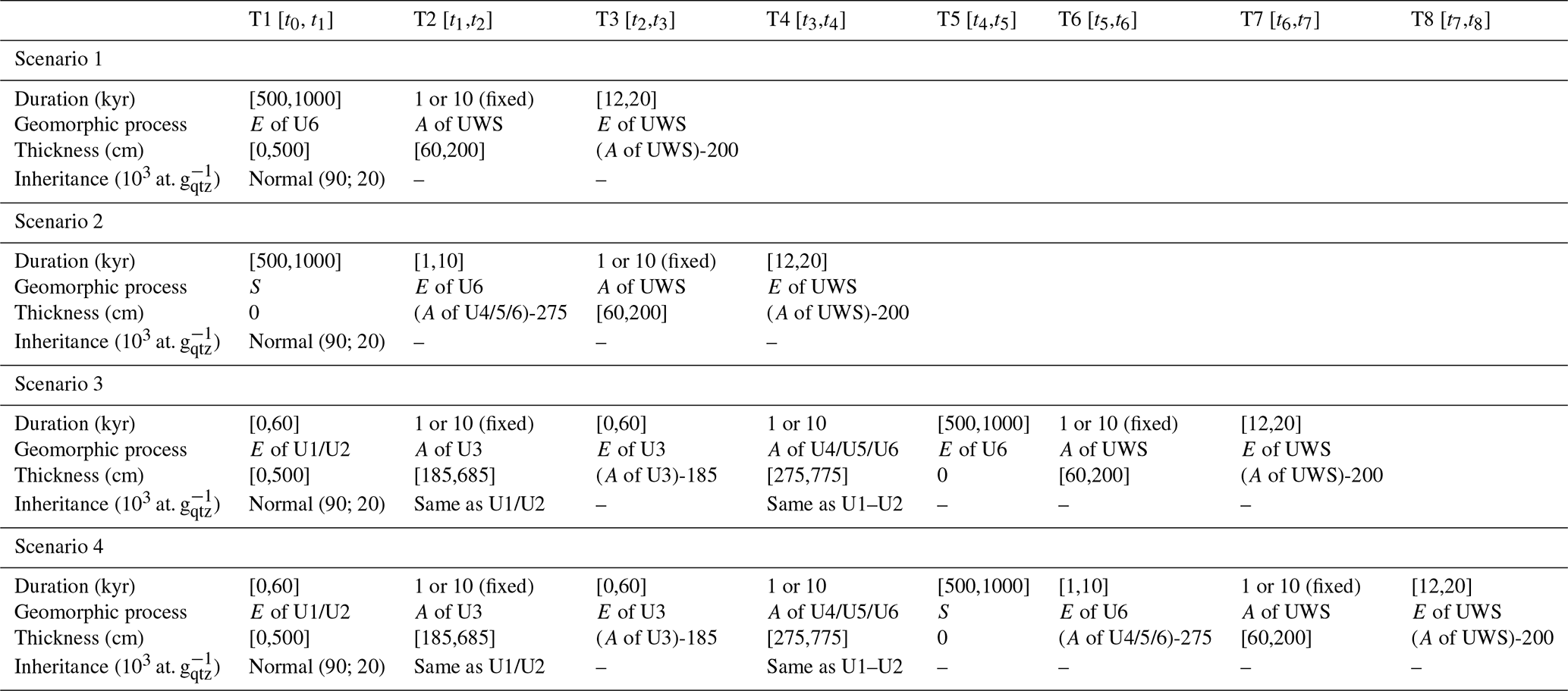
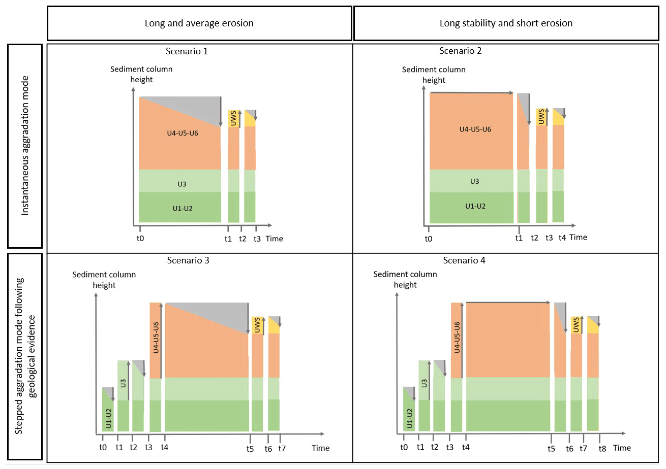
Figure 5 The four scenarios that are developed to represent the sedimentary sequence of the Zutendaal gravels in As. Grey arrows represent aggradation (upward arrow), erosion (downward arrow) or stability (horizontal arrow). The material that is removed by erosion is coloured in grey.

We ran each scenario 10⁷ times with 6.75 as the inherited ²⁶Al $/$ ¹⁰Be ratio and then again 10⁷ times with a ratio of 7.40. The latter is a mean value between the ²⁶Al $/$ ¹⁰Be ratio for production at the surface and the ratio observed at depth by e.g. Margreth et al. (2016). By varying the inherited ²⁶Al $/$ ¹⁰Be ratio, we aim to account for a potential mix of sediments sourced by deep and surface erosion. A plot of kernel-density estimates using Gaussian kernels was then generated from the simulations that were considered to be possible solutions based on their associated reduced χ² value. For each parameter, the value representing the highest density of solutions is given as the optimal model outcome, and the uncertainties are reported with 95 % confidence intervals (2σ).

Based on prior information on the evolution of the Zutendaal gravels, four constraints were defined:

1. “Not longer than”. The total geomorphic history takes place over the last 1000 kyr (Beerten et al., 2018, and references therein). In consequence, any scenario for which the total duration exceeded 1000 kyr was automatically discarded.

2. “Not shorter than”. In the area where the Zutendaal gravels are currently outcropping, deposition ended by 500 ka at the latest (Westerhoff et al., 2008). The abandonment of the terrace must be older than 500 ka.

3. “Final thickness of every unit should correspond to the measured thickness”. After an aggradation phase, the thickness of the unit can decrease by erosion over the following time period until it matches the observed, present-day thickness.

4. The two last time periods of any scenario should include 60 to 200 cm aggradation of Weichselian coversands (unit Weichselian coversands, abbreviated “UWS”), followed by an erosion phase until the thickness of the coversands matches the present-day thickness.

The model was run for each scenario using the constraints and parameter distributions of Table 1. Parameter values were attributed randomly, following Hidy et al. (2010). The two first scenarios, scenarios 1 and 2, represent the classical depth profile (Braucher et al., 2009): scenario 1 represents a long and constant post-depositional erosion phase, whereas scenario 2 represents a long stable phase that is followed by a recent, pre-Weichselian episode of rapid erosion. In scenario 1, the fluvial gravel sheet starts accumulating CRNs over a [500, 1000] kyr period that is characterised by constant erosion of [0, 500] cm. In contrast, in scenario 2, the fluvial sheet remains stable over T1 and then undergoes a rapid erosional phase of [0, 500] cm over 1 or 10 kyr (T2). The maximum erosion rate is thus 500 cm in 1 kyr, or 5 mm yr⁻¹, and is based on the upper range of long-term erosion rates reported in literature (Portenga and Bierman, 2011; Covault et al., 2013). After erosion, the fluvial sheet is covered by Weichselian coversands (UWS) during a 1–10 kyr period. The sand deposit is then eroded until it reaches the present-day thickness of 60 cm. In both scenarios, the onset of the in situ CRN accumulation is concomitant with the beginning of the post-depositional period (Fig. 5).

In contrast to the instantaneous aggradation mode of scenarios 1 and 2, scenarios 3 and 4 consider a stepped aggradation mode and are based on ancillary data from geochemical proxies (Vandermaelen et al., 2022a). As illustrated in Fig. 5, the simulations start with unit U1–U2 in place at the bottom of the sedimentary sequence. This is followed by different phases of aggradation and erosion. The duration of any erosion phase is set to a maximum of 60 kyr so that two erosion phases account for a maximum of 120 kyr. This corresponds to the duration of a full glacial cycle, i.e. about 110 to 120 kyr, based on Busschers et al. (2007). The first phase of erosion of [0, 500] cm is thus simulated over a T1 period of [0, 60] kyr. This is followed by the T2 period with [185, 685] cm aggradation of unit U3. The minimum aggradation corresponds to the present-day thickness of U3 and takes place during a single step, 1 kyr, or 10 kyr (Table 1). During the T3 period, the thickness of U3 that exceeds 185 cm is eroded over [0, 60] kyr. The next aggradation phase, T4, is characterised by [275, 775] cm aggradation of units U4, U5 and U6 over 1 or 10 kyr. The minimum aggradation corresponds to their present-day thickness. After this phase, the post-depositional evolution of the fluvial sequence starts: in scenario 3, the thickness of U4, U5 and U6 that exceeds 275 cm is then slowly and constantly eroded over [500, 1000] kyr, corresponding to the T5 period. In scenario 4, there is a long phase of stability during the T5 period that is then followed by a phase of rapid erosion during the T6 period, lasting [1, 10] kyr. In both scenarios 3 and 4, the last two periods are similar to the aggradation and erosion of the Weichselian coversands specified in scenarios 1 and 2.

3 Results

3.1 In situ-produced CRN concentrations along the depth profile

The ¹⁰Be concentrations vary from 120 × 10³ to more than 200 × 10³ at. g${}_{\mathrm{qtz}}^{-\mathrm{1}}$ (Table 2). The total uncertainties on the measured ¹⁰Be concentrations are below 7 %, with the exception of the lowermost sample (Heras-02). The observed CRN depth variation deviates from a simple exponential decrease of ¹⁰Be concentration with depth and points to a complex deposition history. The upper eight values (70 to 300 cm, corresponding to U6, U5 and U4) show an exponential decrease from (175 ± 8) × 10³ to (122 ± 7) × 10³ at. g${}_{\mathrm{qtz}}^{-\mathrm{1}}$ (Fig. 6). There is an abrupt change in the concentration at 370 cm depth, corresponding to (135 ± 7) × 10³ at. g${}_{\mathrm{qtz}}^{-\mathrm{1}}$ measured at the top of the U3 unit, about 12 % higher than the sample taken at 300 cm depth. The following two samples in U3 show a steady decrease in ¹⁰Be concentration with depth. At the bottom of the profile, in the upper part of U1, a third local maximum of ¹⁰Be concentration is found. The value of (202 ± 8) × 10³ at. g${}_{\mathrm{qtz}}^{-\mathrm{1}}$ measured at 550 cm depth is the highest value that was measured in the profile and is 50 % higher than the average ¹⁰Be concentration measured in the overlying units. The samples taken in U1 show a steady decrease of ¹⁰Be concentration with depth, from (145 ± 8) × 10³ at. g${}_{\mathrm{qtz}}^{-\mathrm{1}}$ at 586 cm to (130 ± 30) × 10³ at. g${}_{\mathrm{qtz}}^{-\mathrm{1}}$ at 657 cm depth.

Table 2 In situ-produced CRN concentrations. All reported uncertainties are 1 standard deviation (1σ).

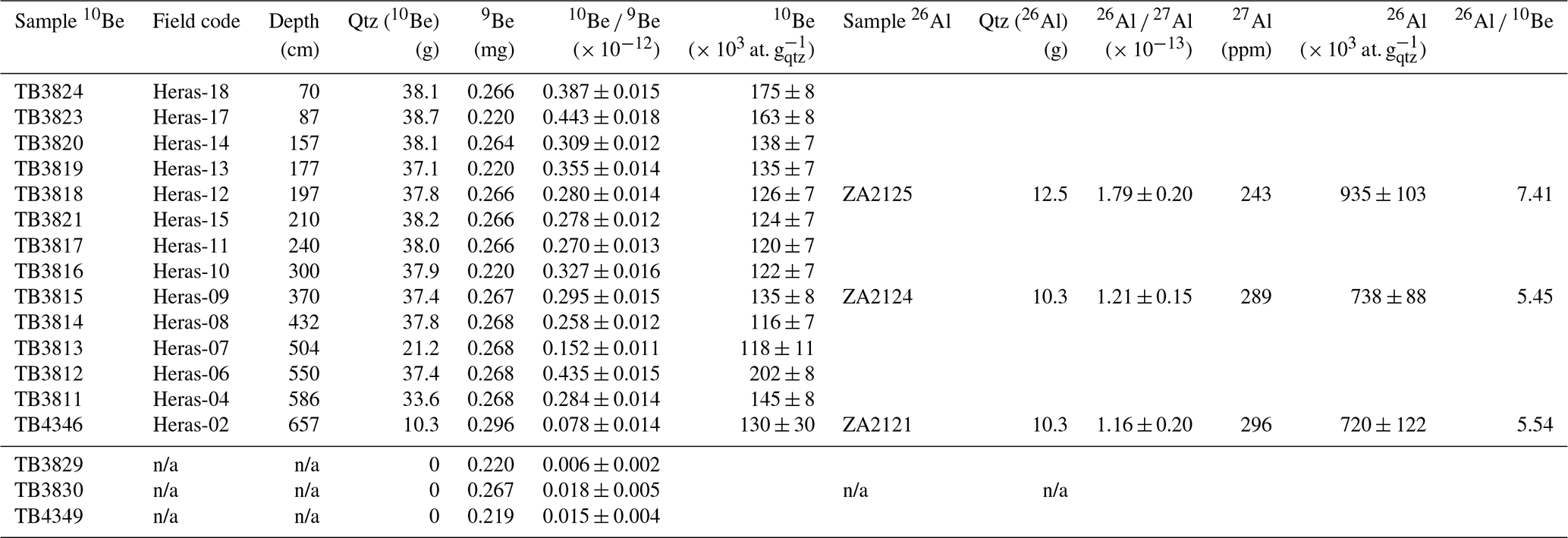
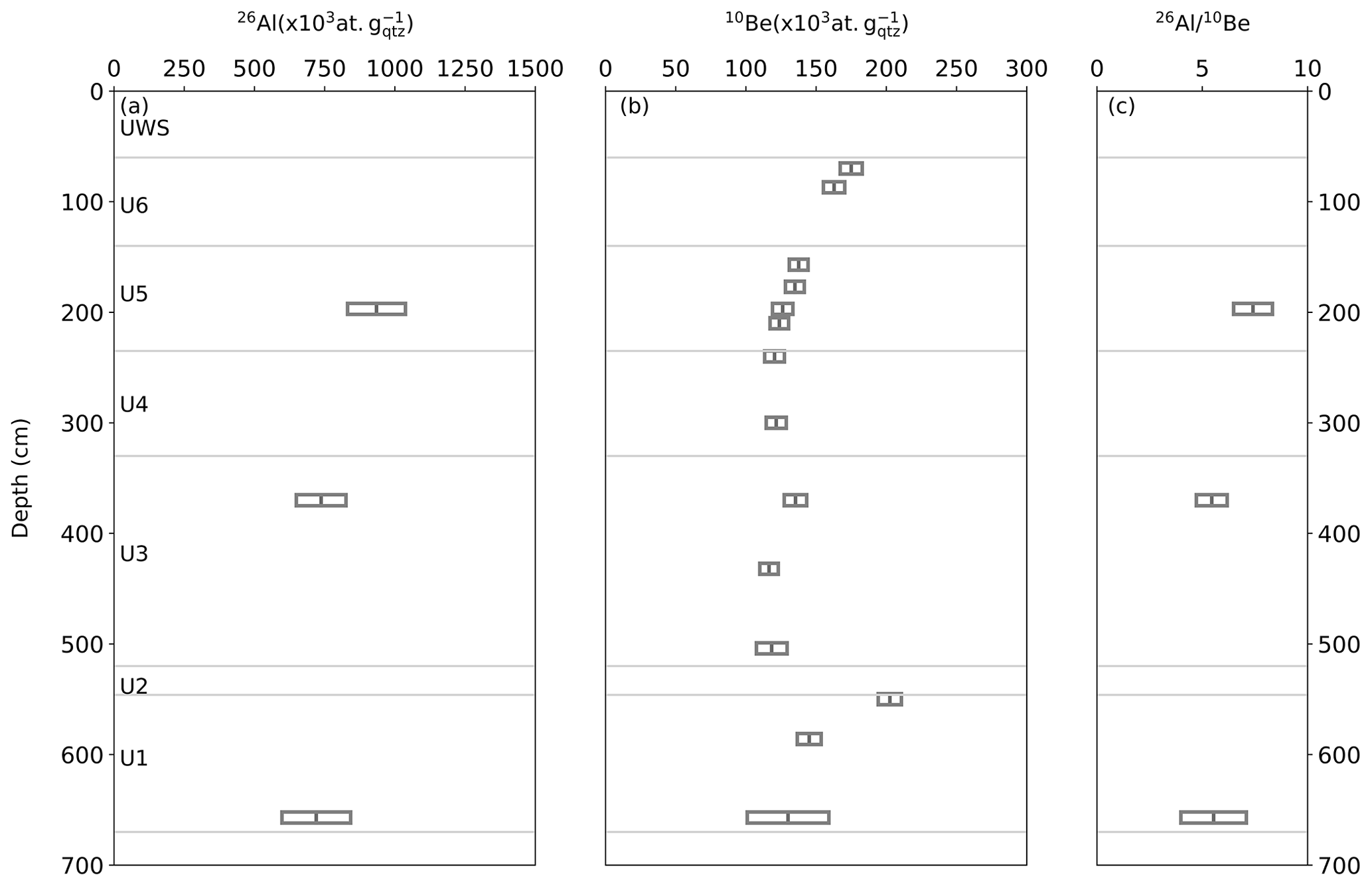
Figure 6 Panels (a) and (b) present the ²⁶Al and ¹⁰Be concentration and (c) the ²⁶Al $/$ ¹⁰Be ratio. The reported uncertainties are 1 standard deviation (1σ).

The three samples analysed for ²⁶Al show a decrease of ²⁶Al concentration with depth: from (934 ± 103) × 10³ at. g${}_{\mathrm{qtz}}^{-\mathrm{1}}$ at 197 cm depth (U5) to (734 ± 88) × 10³ at. g${}_{\mathrm{qtz}}^{-\mathrm{1}}$ at 370 cm depth (U3) and finally to (720 ± 122) × 10³ at. g${}_{\mathrm{qtz}}^{-\mathrm{1}}$ at 657 cm depth (U1). Considering the total uncertainties of 11 % to 17 % on the AMS and ICP-AES measurements, only the ²⁶Al concentration of the uppermost sample is significantly higher than the two deeper ones (Fig. 6). Although based on a limited number of samples, the depth evolution of the ²⁶Al concentrations differs from what is observed for the ¹⁰Be concentrations, as the ¹⁰Be concentration appears higher at 370 cm depth than at 197 cm depth.

The three ²⁶Al $/$ ¹⁰Be ratios decrease with depth, with values of 7.41 ± 0.92 at 197 cm, 5.45 ± 0.73 at 370 cm and 5.54 ± 1.55 at 657 cm. The measured ratios are consistent with near-surface production (i.e. ²⁶Al $/$ ¹⁰Be ratio of 6.75; Granger and Muzikar, 2001; Erlanger et al., 2012).

3.2 Optimal model fits

The optimal model fits for the scenarios representing the instantaneous aggradation mode (i.e. scenarios 1 and 2, Fig. 5) return a minimised reduced χ² value above 11 and fail to represent the observed ¹⁰Be and ²⁶Al data correctly. Best fits for these scenarios are also unsensitive to the inherited ²⁶Al $/$ ¹⁰Be ratio. The optimal model fits for the scenario that consider a stepped aggradational mode and long and average erosion (i.e. scenario 3, Fig. 5) have a reduced χ² value of 130 when using aggradation phases of 1 kyr and 147 using phases of 10 kyr. The goodness of fit does not improve when using an inherited ²⁶Al $/$ ¹⁰Be ratio of 7.40 instead of 6.75 (Table 3).

Table 3 Reduced χ² values of the optimal model fits for scenario 1, 2, 3 and 4, with ²⁶Al $/$ ¹⁰Be ratios of 6.75 and 7.40 and with 1 and 10 kyr durations of the aggradation phases. The star indicates whether the p value did not show a significant disagreement between observed and modelled CRN concentrations.

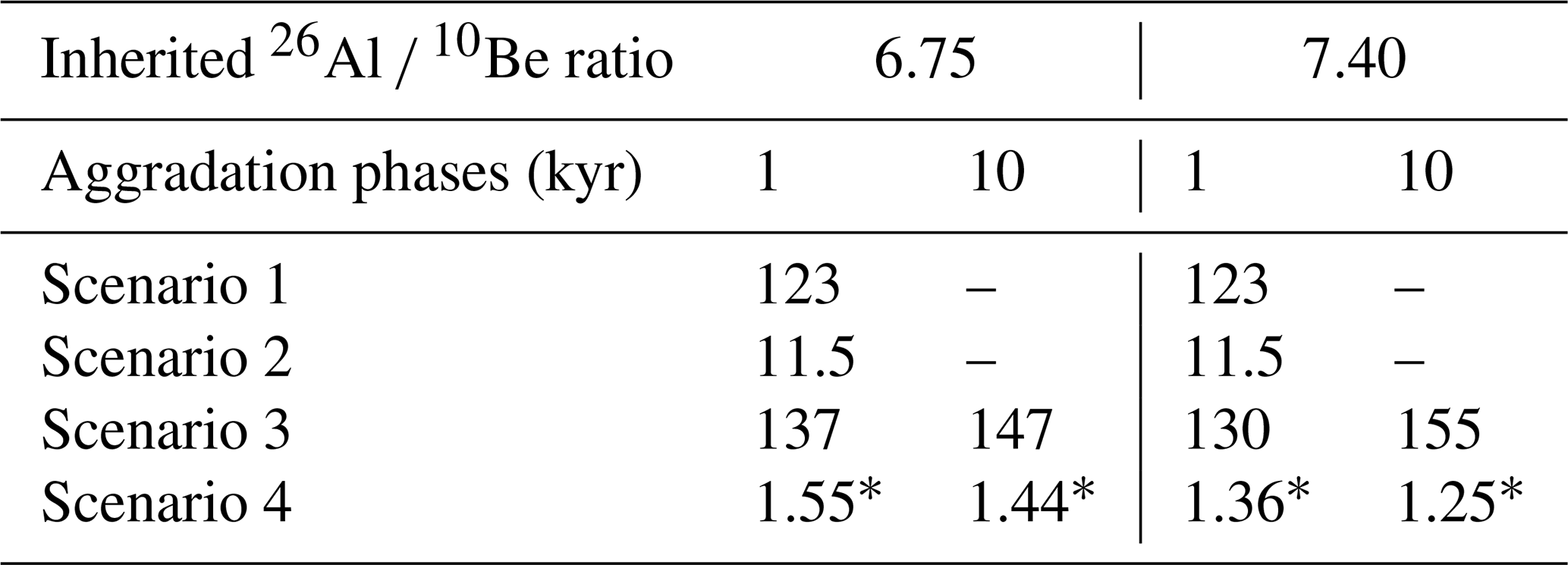
The scenarios that consider a stepped depositional history and a period of [500; 1000] kyr of landscape stability (scenario 4) show better optimal fits (Table 3). At the 0.05 significance level, the simulations can be accepted as possible solutions when the reduced χ² value is below 1.83. With the inherited ²⁶Al $/$ ¹⁰Be ratio of 6.75, the optimal simulations with aggradation phases of 1 and 10 kyr have a reduced χ² value of, respectively, 1.55 and 1.44. The model fit improves when using inherited ²⁶Al $/$ ¹⁰Be ratios of 7.40, with optimal reduced χ² values of, respectively, 1.36 and 1.25. Given that the goodness of fit is similar for the simulations with aggradation phases of 1 or 10 kyr, we pooled all results in the kernel-density plots. Figure 6 resumes the results on the overall aggradation time of the entire sequence; the deposition age of the lowermost unit, U1; and the duration of hiatuses and corresponding surface erosion at the top of the U2, U3 and U6 layers. The optimal values are reported with their 95 % confidence intervals (2σ).

The hiatus at the top of the U2 unit is characterised by a duration of ${\mathrm{44}}_{-\mathrm{7}}^{+\mathrm{15}}$ kyr and an erosion amount of ${\mathrm{17}}_{-\mathrm{17}}^{+\mathrm{56}}$ cm in the simulations with inherited ratios of 6.75 (Fig. 7a) and ${\mathrm{50}}_{-\mathrm{12}}^{+\mathrm{10}}$ kyr and ${\mathrm{23}}_{-\mathrm{23}}^{+\mathrm{56}}$ cm in simulations with inherited ratios of 7.40 (Fig. 7b). The combination of hiatus duration and erosion amount results in an erosion rate of 4.60 and 3.86 m Myr⁻¹ for simulations with inherited ratios of, respectively, 6.75 and 7.40. Although this erosion rate is 1 order of magnitude lower than the median global denudation rate (i.e. 54 m Myr⁻¹) that was calculated from a set of 87 drainage basins (Portenga and Bierman, 2011), it is coherent with the lowest long-term incision rate reported for the Meuse catchment near Liège (Van Balen et al., 2000).

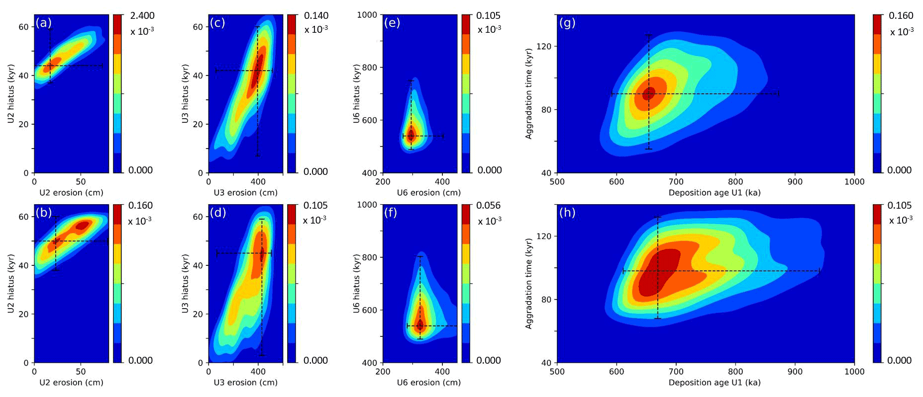
Figure 7 Density plot of the possible model outcomes for scenario 4. Any simulation that returned a reduced χ² smaller than 1.83 is considered to be significant and is included as a possible solution in the density plots. The density of significant solutions is shown by colour coding. The four upper panels (a, c, e, g) represent the parameters of simulations (n = 486) characterised by a ²⁶Al $/$ ¹⁰Be of 6.75, and the lower panels (b, d, f, h) represent the parameters of simulations (n = 1695) with a ²⁶Al $/$ ¹⁰Be of 7.40. For each parameter, the most likely value (i.e. the value with highest density of significant solutions) is reported along with its 95 % confidence interval (2σ). The 95 % confidence interval is derived from the 2.5 % and 97.5 % limits of the kernel cumulative density function.

For the hiatus at the top of U3, the highest density of solutions is observed around ${\mathrm{42}}_{-\mathrm{35}}^{+\mathrm{18}}$ and ${\mathrm{45}}_{-\mathrm{42}}^{+\mathrm{14}}$ kyr for simulations with an inherited ratio of, respectively, 6.75 and 7.40 (Fig. 7c, d), which is similar to the hiatus' duration established for the lower U2 unit. In contrast, the associated solutions for erosion are 1 order of magnitude higher than at the top of U1–U2, with values of ${\mathrm{395}}_{-\mathrm{335}}^{+\mathrm{120}}$ cm (94 m Myr⁻¹) and ${\mathrm{430}}_{-\mathrm{363}}^{+\mathrm{76}}$ cm (96 m Myr⁻¹) for inherited ratios of, respectively, 6.75 and 7.40. The hiatus on top of U6 encloses the time between the last aggradation of fluvial deposits and the Weichselian coversands. The highest density of possible solutions is found at ${\mathrm{540}}_{-\mathrm{52}}^{+\mathrm{209}}$ kyr for simulations with an inherited ratio of 6.75, and a similar value, i.e. ${\mathrm{540}}_{-\mathrm{50}}^{+\mathrm{263}}$ kyr, is found with a ratio of 7.40 (Fig. 7e). The erosion of the overburden that was present on top of U6 took place before the aggradation of Weichselian coversands and is estimated at ${\mathrm{295}}_{-\mathrm{27}}^{+\mathrm{208}}$ and ${\mathrm{325}}_{-\mathrm{43}}^{+\mathrm{151}}$ cm for inherited ratios of, respectively, 6.75 and 7.40 (Fig. 7f). Constant erosion of the overburden over the period of [500; 1000] kyr is not likely (i.e. scenario 3, Table 3), and a scenario with rapid erosion of the overburden results in significantly better model fit (i.e. scenario 4, Table 3). The current model setup fixed the time interval at [1, 10] kyr, which results in optimal values of 295 and 325 m Myr⁻¹. Further research is needed to better constrain the timing and length of such an erosion phase, as they have a strong impact on the erosion estimates.

Based on the CRN age–depth modelling, the deposition age of the bottommost deposits of the exposure was constrained at ${\mathrm{654}}_{-\mathrm{62}}^{+\mathrm{218}}$ and ${\mathrm{669}}_{-\mathrm{58}}^{+\mathrm{272}}$ ka for inherited ratios of, respectively, 6.75 and 7.40 (Fig. 7g, h). The total formation time of the sedimentary sequence, including the aggradation phases and the sedimentary hiatuses, is estimated at ${\mathrm{90}}_{-\mathrm{45}}^{+\mathrm{37}}$ and ${\mathrm{98}}_{-\mathrm{30}}^{+\mathrm{34}}$ kyr for inherited ratios of, respectively, 6.75 and 7.40 (Fig. 7g, h). The top of the Zutendaal Formation that is exposed in As has a deposition age of ${\mathrm{562}}_{-\mathrm{45}}^{+\mathrm{211}}$ and ${\mathrm{565}}_{-\mathrm{44}}^{+\mathrm{269}}$ ka for inherited ratios of, respectively, 6.75 and 7.40.

4 Discussion

4.1 Aggradation mode of the Zutendaal gravels

The onset of aggradation of the Middle Pleistocene gravel deposits of the so-called Main Terrace of the Meuse in NE Belgium, the Zutendaal gravels, was commonly assumed to be situated between 500 and 1000 ka (van den Berg, 1996; Van Balen et al., 2000; Gullentops et al., 2001; Westerhoff et al., 2008). Here, by applying a numerical model to the CRN concentration depth profiles, the age for the onset of U1 aggradation is estimated to be ${\mathrm{654}}_{-\mathrm{62}}^{+\mathrm{218}}$ ka. This age, within error limits, agrees with previous correlations of the gravel sheet with the Cromerian Glacial B and Marine Isotope Stage (MIS) 16 (Gullentops et al., 2001). Around this time, the gravel sheet was already in the process of being built, and only the upper part of the Zutendaal gravels (potentially 15 to 20 m thick gravel sheet) is here exposed. Therefore, it cannot be excluded that the base of the (buried part of the) Zutendaal gravels corresponds with MIS 18.

The model simulations also confirmed the existence of a stepped aggradation mode, whereby phases of aggradation are alternating with phases of stability or erosion. At least three phases of aggradation with two intraformational hiatuses are identified: a first hiatus at the top of the U2 unit lasting ${\mathrm{44}}_{-\mathrm{7}}^{+\mathrm{15}}$ kyr and resulting in surface erosion of ${\mathrm{17}}_{-\mathrm{17}}^{+\mathrm{56}}$ cm; a second hiatus at the top of the U3 unit with similar duration, i.e. ${\mathrm{42}}_{-\mathrm{35}}^{+\mathrm{18}}$ kyr, but much higher surface erosion of ${\mathrm{395}}_{-\mathrm{335}}^{+\mathrm{120}}$ cm. The third and final aggradation phase (U4–U5–U6, ending at last at ${\mathrm{562}}_{-\mathrm{45}}^{+\mathrm{211}}$ ka) occurred before abandonment of the region by the Meuse River. The results are here reported for inherited ratios of 6.75 and aggradation phases of 1 and 10 kyr, but they do not differ significantly when using alternative inherited ²⁶Al $/$ ¹⁰Be ratios (Table 3).

The total formation time of the sedimentary sequence exposed in As is estimated at ${\mathrm{90}}_{-\mathrm{45}}^{+\mathrm{37}}$ kyr. Given that only the upper 7 m are exposed in As (Gullentops et al., 2001), the deposition of the entire sequence of the Zutendaal gravels probably represents more than one climatic cycle. Slow aggradation leading to ¹⁰Be enrichment with depth (e.g. Nichols et al., 2002; Rixhon et al., 2014) is not directly observed in this sequence. However, it could eventually have occurred in the shallow and sandy unit, U2, that was not sampled for ¹⁰Be. Slow aggradation would further increase the total formation time. Such a prolonged formation time can occur in fluvial depositional systems in the absence of tectonic uplift and consecutive river downcutting (Sougnez and Vanacker, 2011). Only after the Meuse River abandoned its northwestern course (Fig. 1) did it develop a staircase of alluvial terraces in response to tectonic uplift of the Ardennes–Rhenish Massif (Beerten et al., 2018 and references therein).

According to simulations of scenario 4, an overburden remained in place from the abandonment time until it was removed by an erosion phase, which preceded the sedimentation of the Weichselian aeolian cover. Other scenarios could be tested, whereby the post-depositional history is characterised by alternating phases of aeolian sand deposition and subsequent removal of this loose material (Beerten et al., 2017). The aeolian sand deposits that cover the top of various Meuse River terraces in the northern part of the Meuse Valley are commonly assumed to be Weichselian in age (e.g. Vanneste et al., 2001; Derese et al., 2009; Vandenberghe et al., 2009) regardless of their morphological position and age (Paulissen, 1973). This being said, a few very thin Late Saalian aeolian sand deposits were found on top of the Saalian Eisden-Lanklaar terrace near the steep valley wall of the Meuse River east of the study site (Paulissen, 1973). This would imply that only the latest episode of sand movement is well preserved on the top of the terrace landscape and previous aeolian sand covers have been reworked during subsequent glacial–interglacial cycles that followed the deposition of the terrace deposits.

4.2 Added value of modelling complex aggradation modes

Studies using the classical CRN depth profile approach mainly envision delivering an exposure age of the surface, i.e. of the uppermost deposits only. By using numerical modelling, it becomes possible to reconstruct the aggradation time and mode of a sedimentary sequence based on the evolution of the CRN concentrations with depth. This case study in NE Belgium demonstrates that the total formation time of braided-river deposits, such as the Zutendaal gravels, may constitute nearly 20 % of the deposition age (Fig. 7g, h). This shows the importance of considering the aggradation mode of braided rivers when applying CRN techniques to > 3 m deep sedimentary sequences.

Firstly, this approach can account for the presence of hiatuses in the sedimentary sequence. Hiatuses in the aggradation process temporarily expose parts of fluvial sheets that would otherwise be buried at depth and partially shielded from CRN accumulation. This can create a positive offset in the CRN concentration depth profile, whereby the concentration at a given depth is higher than the true inheritance value (Fig. 6; Vandermaelen et al., 2022a). Such observations do not fit in the simple concentration depth distribution and are often classified as outliers or as results of differential inheritance (e.g. following the concepts reported by Le Dortz et al., 2011).

Secondly, by considering the aggradation mode, additional information on the sourcing of sediments can be extracted from the depth distribution of ²⁶Al $/$ ¹⁰Be ratios. The ²⁶Al $/$ ¹⁰Be ratios that are measured in fluvial sediments result from (i) the inherited ²⁶Al $/$ ¹⁰Be ratios of the source material and (ii) the in situ CRN accumulation when the material is exposed to cosmic rays. Accounting for the changing depth of the sedimentary layers within the fluvial sheet may allow one to explain high ²⁶Al $/$ ¹⁰Be ratios (i.e. > 6.75) measured at depth. For the case study in NE Belgium, the model fit improved slightly when an inherited ²⁶Al $/$ ¹⁰Be ratio of 7.40 was used in the simulations (Fig. 7). Inherited ²⁶Al $/$ ¹⁰Be ratios that are substantially higher than 6.75 often point to intense physical erosion in the headwater basins where material is sourced from deep erosion by e.g. (peri)glacial processes (Claude et al., 2017; Knudsen et al., 2019). The material that was buried several metres below the surface is then delivered to the fluvial system and breaks into smaller parts on its route to the final sink or during intermediate storage. Such deposits are then constituted of a mix of sediments characterised by different ²⁶Al $/$ ¹⁰Be inherited ratios. In their final sink, the sediments will further accumulate CRN following the ²⁶Al $/$ ¹⁰Be surface production ratio of ∼ 6.75 when exposed at (or close to) the surface, or they can maintain an ²⁶Al $/$ ¹⁰Be isotope ratio above 6.75 when quickly buried to a depth above 300 g cm⁻², where the relative production of ²⁶Al to ¹⁰Be is larger due to muogenic production.

4.3 Trade-off between model complexity and sample collection

Optimisation methods like the reduced χ² require that the number of observed data is larger than the number of free parameters (Hidy et al., 2010). There is thus a trade-off to make between the complexity of the model and the number of data points obtained by CRN analyses. In case of CRN concentration depth profiles, the number of samples is often limited by the capacity and financial constraints that are needed to process samples for CRN analyses. In the numerical model, the phases of aggradation are characterised by their duration, aggradation thickness and inherited ¹⁰Be concentration. They are followed by phases of stability or erosion with an unknown duration.

The inclusion of aggradation modes in CRN concentration depth profile modelling therefore requires more unconstrained parameters than the classical depth profile approach (Table 1). The minimum number of CRN measures that is required can be calculated as follows:

$$\begin{array}{}\text{(4)}& N_{\mathrm{CRN}}>(k\times N_{\mathrm{aggrad}})+(l\times N_{\mathrm{erosion}}),\end{array}$$

where N_CRN is the number of CRN measurements for individual samples; k and l are the number of unconstrained parameters for, respectively, each aggradation and erosion or stability phase. Further complexification of the model by e.g. including unconstrained parameters for sediment density or ²⁶Al $/$ ¹⁰Be inherited ratio will further increase the required number of CRN observations. With a limited number of samples, the complexity of the model can be reduced by, e.g. keeping the CRN inheritance fixed. This is acceptable when the local minima of the CRN concentrations in a given sedimentary sequence are within 10 % of the mean of the lowest values. For braided-river deposits, it is also viable to fix the length of the aggradation phase to 1 or 10 kyr: most sedimentary sequences represent long periods of non-deposition or erosion interrupted by rapid and short-lived depositional events (Bristow and Best, 1993).

4.4 Chronostratigraphical implications

Based on the age of ${\mathrm{654}}_{-\mathrm{62}}^{+\mathrm{218}}$ ka obtained for the base of the sedimentary sequence in As, the Zutendaal gravels exposed at the geosite in As were most likely deposited during MIS 16, and the lower part maybe even during MIS 18, according to northwest European chronostratigraphical subdivision and correlation with the marine isotope record (Cohen and Gibbard, 2019). The uppermost part of the deposits (U6, Fig. 6) in As is dated at ${\mathrm{562}}_{-\mathrm{45}}^{+\mathrm{211}}$ ka, thereby yielding a youngest possible deposition age of 517 ka. This age would associate the uppermost deposits with MIS 14. However, it cannot be ruled out that, by that time, the Meuse had already shifted its course towards the east of the As sampling site (Van Balen et al., 2000). If this is true, the uppermost depositional sequence in As should correspond to material deposited by another local river rather than by the Meuse itself. It is possible that the Bosbeek occupied this part of the Campine Plateau after the Meuse had shifted to the east. A fossil valley floor of the Bosbeek River has been identified by Gullentops et al. (1993), only a few hundred metres away from the As sampling site.

The absolute dating of the Zutendaal gravels contributes to constraining the chronostratigraphical framework of the Campine Plateau and the Meuse River terraces. Several authors (e.g. Pannekoek, 1924; Paulissen, 1973) have formulated the hypothesis that the Zutendaal gravels may represent the Main Terrace in the part of the Meuse Valley downstream of Maastricht. However, the correlation between terrace fragments located at different locations along the Meuse River is still a subject of scientific debate. However, it remains interesting to compare the chronological framework of the Zutendaal gravels on top of the Campine Plateau with the younger Main Terrace levels of the Meuse River in the Liège area and the Ardennes. van den Berg (1996) used paleomagnetic techniques on the different sub-levels of the Sint-Pietersberg Terrace to obtain age estimates of the Main Terrace in the region of Maastricht. The age of the uppermost sub-level was estimated at 955 ka by van den Berg (1996) and at 720 ka by Van Balen et al. (2000) based on the same data. Both studies agree on an age of 650 ka for the next sub-level. Rixhon et al. (2011) dated the younger Main Terrace of the Meuse River in the locality of Romont, ∼ 25 km upstream of our sampling position, using in situ-produced ¹⁰Be depth profiles. They obtained an age of 725 ± 120 ka (mean ± 1 SD). Although this age is somewhat older than the top of the Zutendaal gravels that we dated with CRN depth modelling (i.e. ${\mathrm{562}}_{-\mathrm{45}}^{+\mathrm{211}}$ ka, optimal solution with 95 % CI), it is not inconsistent, as it overlaps with the CRN optimal solution considering the 95 % confidence interval.

5 Conclusion

The aggradation and preservation modes of Middle Pleistocene braided-river deposits were studied here based on in situ cosmogenic radionuclide concentrations. To account for potential discontinuous aggradation, a numerical model was developed to simulate the accumulation of cosmogenic radionuclides, ¹⁰Be and ²⁶Al, in a sedimentary sequence and to account for deposition and erosion phases and post-depositional exposure. The method was applied to the Zutendaal gravels outcropping in NE Belgium, and 17 sediment samples were taken over a depth of 7 m and processed for determination of ¹⁰Be and ²⁶Al concentrations. The model parameters were optimised using reduced χ² minimisation. The Zutendaal gravels were deposited during (at least) three superimposed aggradational phases that were interrupted by stability or erosion lasting ∼ 40 kyr. This illustrates how long periods of non-deposition alternate with rapid and short depositional events. The key chronostratigraphical outcomes of this study, based on the optimal model outcomes, are as follows: (1) the fluvial deposits found at 7 m depth in As are dated at ${\mathrm{654}}_{-\mathrm{62}}^{+\mathrm{218}}$ ka, thereby corresponding to MIS 16; (2) the uppermost sequence of these deposits is dated at ${\mathrm{562}}_{-\mathrm{45}}^{+\mathrm{211}}$ ka, corresponding to MIS 14 and thereby possibly deposited by another stream apart from the Meuse River, which is assumed to have shifted its course east by that time; and (3) the total formation time of the upper 7 m of the Zutendaal gravels in As is about 90 kyr, so the deposition of the entire gravel sheet could correspond to more than one glacial period. The total formation time of the Zutendaal gravels constitutes nearly 20 % of the deposition age and shows the importance of considering the aggradation mode of braided rivers when applying CRN techniques to > 3 m deep sedimentary sequences.